de Bordeaux 18(2006), 487–536
Unimodular Pisot substitutions and their
associated tiles
parJ¨org M. THUSWALDNER
Dedicated to Professor Helmut Prodinger on the occasion of his 50th
birthday
R´esum´e. Soit σ une substitution de Pisot unimodulaire sur un alphabet `a d lettres et soient X1, . . . , Xd les fractales de Rauzy
associ´ees. Dans le pr´esent article, nous souhaitons ´etudier les fronti`eres ∂Xi (1 ≤ i ≤ d) de ces fractales. Dans ce but, nous
d´efinissons un graphe, appel´e graphe de contact de σ et not´e C. Siσsatisfait une condition combinatoire appel´eecondition de su-per co¨ıncidence, le graphe de contact peut ˆetre utilis´e pour ´etablir un syst`eme auto-affine dirig´e par un graphe dont les attracteurs sont des morceaux des fronti`eres ∂X1, . . . , ∂Xd. De ce syst`eme
dirig´e par un graphe, nous d´eduisons une formule simple pour la dimension fractale de∂Xi, dans laquelle les valeurs propres de la matrice d’adjacence deCinterviennent.
Un avantage du graphe de contact est sa structure relativement simple, ce qui rend possible sa construction imm´ediate pour une grande classe de substitutions. Dans cet article, nous construisons explicitement le graphe de contact pour une classe de substitu-tions de Pisot qui sont reli´ees auxβ-d´eveloppements par rapport `a des unit´es Pisot cubiques. En particulier, nous consid´erons des substitutions de la forme
σ(1) = 1. . .1 | {z }
bfois
2, σ(2) = 1. . .1 | {z }
afois
3, σ(3) = 1
o`u b≥a≥1. Il est bien connu que ces substitutions satisfont la condition de super co¨ıncidence mentionn´ee plus haut. Donc nous pouvons donner une formule explicite pour la dimension fractale des front`ıeres des fractales de Rauzy associ´ees `a ces substitutions.
Abstract. Let σ be a unimodular Pisot substitution over a d
letter alphabet and letX1, . . . , Xd be the associated Rauzy
frac-tals. In the present paper we want to investigate the boundaries
∂Xi (1 ≤ i ≤ d) of these fractals. To this matter we define a certain graph, the so-called contact graph C of σ. If σ satisfies
Manuscrit re¸cu le 17 novembre 2004.
a combinatorial condition called the super coincidence condition the contact graph can be used to set up a self-affine graph di-rected system whose attractors are certain pieces of the bound-aries∂X1, . . . , ∂Xd. From this graph directed system we derive an
easy formula for the fractal dimension of∂Xiin which eigenvalues of the adjacency matrix ofC occur.
An advantage of the contact graph is its relatively simple struc-ture, which makes it possible to construct it for large classes of substitutions at once. In the present paper we construct the con-tact graph explicitly for a class of unimodular Pisot substitutions related toβ-expansions with respect to cubic Pisot units. In par-ticular, we deal with substitutions of the form
σ(1) = 1. . .1 | {z }
btimes
2, σ(2) = 1. . .1 | {z }
atimes
3, σ(3) = 1
whereb≥a≥1. It is well known that these substitutions satisfy the above mentioned super coincidence condition. Thus we can give an explicit formula for the fractal dimension of the boundaries of the Rauzy fractals related to these substitutions.
1. Introduction
In 1982 Rauzy [34] studied the Tribonacci substitution
σ(1) = 12, σ(2) = 13, σ(3) = 1.
He proved that the dynamical system generated by this substitution is measure-theoretically conjugate to an exchange of domainsX1, X2, X3 in a
compact tileX=X1∪X2∪X3. The setX has fractal boundary. However,
it is homeomorphic to a closed disk (cf. [30, Subsection 4.1]). Furthermore, the essentially disjoint basic tiles X1, X2, X3 satisfy a self-similar graph directed system in the sense of Mauldin and Williams [28]. The set X is now called theclassical Rauzy fractal.
More generally, it is possible to attach a Rauzy fractal to each unimodular Pisot substitution. However, the structure of these fractals is more compli-cated in the general case. Arnoux and Ito [6] (compare also [4, 5, 11, 12, 40]) proved that the dynamical system associated to a unimodular Pisot sub-stitution over a d letter alphabet admits a conjugacy to an exchange of domainsX1, . . . , Xdin the compact setX =X1∪. . .∪Xd provided that a
certain combinatorial condition, the so-calledstrong coincidence condition is true. It is conjectured that this condition holds for each unimodular Pisot substitution. The topological structure of X can be difficult. There exist substitutions over three letters whose Rauzy fractals are neither connected nor simply connected.
is via certain projections of a set of points related to a periodic point of
σ (see for instance [20, Chapter 8]). Another approach runs via so-called one dimensional “geometric realizations” ofσ and makes use of the duality principle of linear algebra (cf. [6]). Furthermore, Mosse [31] defined a certain “desubstitution map” on the dynamical system Ω associated to σ. With help of this map we can define a graph (the prefix-suffix automaton) that reveals a certain affinity property of Ω. This reflects to a self-affinity property of the Rauzy fractal X which allows to define X by a graph directed system. This graph directed system is satisfied by the basic tiles X1, . . . , Xd and is directed by the prefix-suffix automaton. All these definitions are equivalent and will be reviewed in Sections 2 and 3.
The fractal structure of the boundary of Rauzy fractals has been in-vestigated firstly by Ito and Kimura [24]. They calculated the Hausdorff dimension of the boundary of the classical Rauzy fractal. Recently, Feng et al. [19] gave estimates for the Hausdorff dimension of Rauzy fractals associ-ated to arbitrary unimodular Pisot substitutions. The approach used by Ito and Kimura in their dimension calculations makes use of two dimensional geometric realizations of the Tribonacci substitution. This construction has been considerably generalized and extended in Sano et al. [35] where a kind of Poincar´e duality is established for higher dimensional geometric realizations of substitutions and their duals. Messaoudi [29, 30] studied geometric and topological properites of the classical Rauzy fractal.
Ito and Rao [25] investigate unimodular Pisot substitutions that admit the definition of tilings (see also Thurston [42]). In their paper they describe three different types of tilings which one can obtain using translates of basic tiles of Rauzy fractals. The existence of these tilings again depends on a combinatorial condition, the so-called super coincidence condition. Up to now it is not known whether this condition is satisfied for all unimodular Pisot substitutions or not. The tilings considered in [25], especially the aperiodic one, form the starting point of the present paper. We want to extend the notion of contact matrix (cf. [22]) and contact graph (cf. [37]) to the case of Rauzy fractals in order to study their boundaries. To this matter we use the above mentioned prefix-suffix automaton. In detail, this paper has the following aims.
In Section 2 we recall basic notations and give different equivalent def-initions of the Rauzy fractal X = X1 ∪. . .∪Xd associated to a given
unimodular Pisot substitution σ over a d letter alphabet. Furthermore, we give relations between substitutions and a well-known notion of radix representations, the β-expansions. At the end of this section we define a tiling induced by translates of the basic tiles of a Rauzy fractal.
discussion of the contact graph and illustrate it by some examples. In the setting of self-affine lattice tiles, the contact graph and its adjacency matrix (the contact matrix) have been used in order to derive tiling properties of these tiles and to investigate their boundaries (cf. [22, 37]).
From Section 4 onwards we assume that the substitutions under consid-eration satisfy the super coincidence condition (cf. Definition 4.1). We use the contact graph in order to represent the boundaries ∂X and ∂Xi of a
Rauzy fractalX =X1∪. . .∪Xdas a graph directed system (Theorem 4.3).
In Feng et al. [19] as well as Siegel [39] other graph directed systems for the boundary of Rauzy fractals are given. However, it turns out that our construction is simpler than theirs and can be used to characterize the boundaries of whole classes of Rauzy fractals.
In Section 5 the above mentioned representation of ∂Xi (1 ≤ i ≤ d)
is used to derive an easy formula for the box counting dimension of ∂X
in which eigenvalues of the contact matrix occur (Theorem 5.9). In some cases we can even prove that the box counting dimension agrees with the Hausdorff dimension.
The main advantage of the contact graph is its relatively easy shape. In Section 6 we will calculate the contact graph for the substitutions
σ(1) = 1. . .1
| {z }
btimes
2, σ(2) = 1. . .1
| {z }
atimes
3, σ(3) = 1
where b ≥ a ≥ 1. It turns out that it has roughly the same shape for each substitution from this class (cf. Theorem 6.4). The knowledge of the contact graphs of these substitutions enables us to establish an explicit formula for the Hausdorff dimension of the boundary of the associated Rauzy fractals (cf. Theorem 6.7).
The calculation of the fractal dimension of∂X and ∂Xi is not the only
possible application of the contact graph. In a forthcoming paper we will apply it in order to set up an algorithm which decides whether a given sub-stitution satisfies the above mentioned super coincidence condition. Also the problem of addition inβ-expansions seems to be related to the contact graph.
2. Basic notions
2.1. Substitutions. For d≥2 set A:= {1, . . . , d}. Let A∗ be the set of all finite words on the alphabetA and let AZ
be the set of doubly infinite sequences. As usual, AZ
shall carry the product topology of the discrete topology onA. Thecylinder sets
[u1.u2] :={w= (. . . w−1.w0w1. . .) :w−|u1|. . . w−1.w0w1. . . w|u2|−1=u1.u2}
(u1, u2 ∈ A∗) form a basis of this topology (if u
1 is empty the cylinder set
Asubstitutionσis an endomorphism of the free monoidA∗which satisfies limn→∞|σn(i)|=∞for at least onei∈ A. A substitution naturally extends toAZ
by setting
σ(. . . w−2w−1.w0w1w2. . .) :=. . . σ(w−2)σ(w−1).σ(w0)σ(w1)σ(w2). . . .
The adjacency matrix ofσ is the d×dmatrix defined by
E0(σ) := (aij)
whereaij is the number of occurrences of the letteriinσ(j). If E0(σ) is a
primitive matrix, we call σ a primitive substitution.
Substitutions give rise to certain dynamical systems. Fundamental prop-erties of these dynamical systems are surveyed in Queff´elec [33]. Here we only need some simple facts about them. Letσ be a substitution. We say that a doubly infinite sequence w is a periodic point of σ if there exists a positive integerkwithσk(w) =w. If we can choosek= 1 thenwis called a fixed pointof σ. In Queff´elec [33] it is shown that each substitution has at least one periodic point. Let τ be the shift map on AZ
. It is defined by τ((wi)i∈Z) = (wi+1)i∈Z. A sequence w ∈ AZ with τk(w) = w is called
τ-periodic (k ∈ N). The language L(w) of w ∈ AZ
is the set of all finite words occurring inw. Let Ω(w) :={w′ ∈ AZ
: L(w′) ⊆L(w)}. Then the pair (Ω(w), τ) is called the dynamical system generated byw.
Letσ be primitive. Then Ω := Ω(w) is the same for each periodic point
wof σ. Thus we call (Ω, τ) thedynamical system generated by σ.
Definition 2.1. Let σ be a substitution with adjacency matrix E0(σ). If the characteristic polynomial ofE0(σ)is the minimal polynomial of a Pisot number λ, we call σ a Pisot substitution. If λ is even a unit, we call σ a unimodular Pisot substitution.
In the present paper we will frequently use two very well known examples of unimodular Pisot substitutions in order to illustrate our results. The Fibonacci substitution, which is defined by
σ(1) = 12, σ(2) = 1 and theTribonacci substitution
σ(1) = 12, σ(2) = 13, σ(3) = 1.
The matrix E0(σ) has the form
E0(σ) =
1 1 1 0
and E0(σ) =
1 1 1 1 0 0 0 1 0
for the Fibonacci and Tribonacci substitution, respectively.
unimodular Pisot substitutions. For the case of Pisot substitutions which are not unimodular we refer to Berth´e and Siegel [9] as well as Siegel [38], where some of their properties are discussed.
Holton and Zamboni [23] showed that each fixed point of a Pisot substi-tutionσ is notτ-periodic. Thus the dynamical system (Ω, τ) generated by
σ is infinite.
2.2. The prefix-suffix automaton. The shift space Ω of a primitive substitution is recognizable by a finite automaton. This automaton can be constructed with help of thedesubstitution mapθwhich we will define now (cf. Moss´e [31]). In [31] it is shown that each w = (wℓ)ℓ∈Z ∈ Ω admits a unique representation of the shape w = τkσ(y) with y = (yℓ)ℓ∈Z ∈ Ω and 0 ≤ k < |σ(y0)|. Thus each w may be written in the form w =
. . . σ(y−1)σ(y0)σ(y1). . . with σ(y0) = w−k. . . w−1.w0. . . wl. We use the
notations
p=w−k. . . w−1 (prefix ofσ(y0)),
s=w1. . . wl (suffix of σ(y0)).
Note that w is completely defined by y and the decomposition of σ(y0).
Let
P :={(p, i, s)∈ A∗× A × A∗: there existsj ∈ Asuch thatσ(j) =pis} be the set of all possible decompositions ofσ(y0). According to the above
construction define thedesubstitution map θand thepartition map γ by
θ: Ω→Ω, w7→y such that w=τkσ(y) and 0≤k <|σ(y0)|, γ : Ω→ P, w7→(p, w0, s) such that σ(y0) =pw0sand k=|p|.
With help of these maps we define the prefix-suffix developmentof w∈Ω by the map
G(w) = (γ(θℓw))ℓ≥0 = (pℓ, iℓ, sℓ)ℓ≥0.
Related to this map is the following automaton.
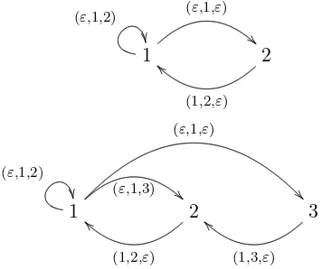
Definition 2.2. The prefix-suffix automatonΓσ associated to a substitution σ has
• Set of states A. Each of the states is an initial state. • Set of labels P.
• There exists an edge from ito j labelled by e= (p, i, s) if and only if
σ(j) =pis.
1
(ε,1,2)
(ε,1,ε)
2
(1,2,ε)
`
`
1
(ε,1,2)
(ε,1,3) (ε,1,ε)
2
(1,2,ε)
`
` 3
(1,3,ε)
`
`
Figure 1. The prefix-suffix automata corresponding to the Fibonacci (above) and the Tribonacci substitution (below).
Let D ⊂ PN
be the set of labels of infinite walks in Γσ. According to
[11] the map Gis continuous and maps onto D. It is one-to-one except at the orbit of periodic points ofσ. This implies that the sets
τkσ[i] (i∈ A, k <|σ(i)|)
partition Ω with countable overlap (cf. [11, Proposition 6.2]). For each
i∈ Awe get the decomposition
(2.1) [i] = [
j∈A,(p,i,s)∈P
σ(j)=pis
τ|p|σ[j].
An analogous representation can be obtained for suffixes. Just note that forσ(j) =piswe have τ|p|σ[j] =τ−|s|−1σ[j.]. Thus (2.1) implies
(2.2) [i.] = [
j∈A,(p,i,s)∈P
σ(j)=pis
τ−|s|σ[j.].
2.3. Construction of the Rauzy fractal. Our first aim is to define a tile X related to a unimodular Pisot substitution σ. Such a tile was first defined for the Tribonacci substitution by Rauzy [34]. First we need the abelianization f of σ. It is defined as follows. Let ei be the canonical i-th
basis vector of Rd. Then
f :A → Zd,
The domain of f is extended to A∗ in the following way. Let w =
be a basis ofCd of right eigenvectors. Then we can select a basis
VC:={v=v1 ≥1, v2, . . . , vr, vr+1,v¯r+1, . . . , vr+s,¯vr+s}
of left eigenvectors such thatUC and VC are dual bases, i.e. ifk= 1, . . . , r
In [12, Lemma 2.4] it is shown that
{u1, u2, . . . , ur,ℜur+1,ℑur+1, . . . ,ℜur+s,ℑur+s}
forms a basis ofRd. This basis is used to define the contracting invariant hyperplane
LetE0(σ)|Pbe the restriction of the linear operatorE0(σ) to the contractive
hyperplanePand set Σr+k=
ℜλr+k ℑλr+k
−ℑλr+k ℜλr+k
(1≤k≤s).
In what follows we identifyC with R2 via the mapping z7→ (ℜz,ℑz) and {0} ×Rd−1 with Rd−1 via the mapping (0, z1, . . . , zd−1) 7→ (z1, . . . , zd−1). Then there exists a regular real matrix TP such that E0(σ)|P = TP−1ΛTP
with
Λ = diag (λ2, . . . , λr,Σr+1, . . . ,Σr+s)
and πf =TP−1δ holds. Now we set
Xi :=TP−1ψ([i]) (i∈ A),
X := [
i∈A
Xi.
Xi(i∈ A) andXare compact subsets of the contracting hyperplaneP. We
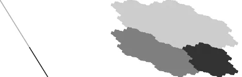
call these sets theatomic surfacesor theRauzy fractalsofσ. In Figure 2 the atomic surfaces of the Fibonacci and Tribonacci substitution are depicted.
Figure 2. The atomic surfaces associated to the Fibonacci (left) and the Tribonacci (right) substitution.
The setsXi (i∈ A) will form the prototiles in the tiling we are going to
define. We mention also the following alternative definition of X and Xi.
Letw= (wℓ)∈Ω be a periodic point of σ. Then
Xi =−{πf(w1. . . wk) : k≥0, wk=i} (i∈ A), X =−{πf(w1. . . wk) : k≥0}.
In Proposition 3.1 we will show that this definition agrees with the definition ofXi and X given above.
Another possibility to define the setsXiruns via graph directed systems.
E its set of edges. To each edgeǫ∈ E assign a contractive affine mapping
where the union is extended over all edgesǫofGstarting ati. The relations (2.4) are called agraph directed system. If the mappingsξǫ are similarities,
we callA=A1∪. . .∪Aq a graph directed self-similar set. The non-empty
compact setsA1, . . . , Aq are uniquely defined by the graph directed system
in (2.4). This can be shown with help of a fix point argument. For a detailed account on graph directed sets we refer the reader to [28].
Observe thatψis one-to-one almost everywhere on each cylinder [i.] (cf. [12, Proposition 4.4]). Now (2.2) yields the following self-affinity property of the sets Xi.
on P, (2.5) is a graph directed system and can be taken as the definition ofXi (i∈ A). ThusX is a graph directed self-affine set.
For the Fibonacci substitution the set equation (2.5) reads
X1 =
for the Tribonacci substitution we get the system
X1=
It has been shown by Sirvent and Wang [40, Theorem 4.1] that Xi has
non-empty interior for each i ∈ A. In fact, they even proved that Xi =
int(Xi).
We want to sum up the results discussed previously in the following proposition.
Proposition 2.3. Let σbe a unimodular Pisot substitution ofdletters and letXi (i∈ A) andX=X1∪. . .∪Xdbe the associated Rauzy fractals. Then
by the graph directed system
Xi =
[
(p,i,s),j
i−−−→(p,i,s) j
E0(σ)Xj+πf(s).
Furthermore,X and Xi are regular sets in the sense that
X= int(X) and Xi= int(Xi) (i∈ A).
2.4. Relations to β-expansions. Atomic surfaces are strongly related to β-expansions of real numbers with respect to a Pisot unit. For a real numberβ >1 we define theβ-transformation
Tβ : [0,1] → [0,1), x 7→ βxmod 1.
Theβ-expansion ofx∈[0,1] is defined by
x=X
ℓ≥1
uℓβ−ℓ
where the “digits”uℓ ∈ {0,1, . . . ,⌈β⌉ −1} are given by uℓ :=⌊βTβℓ−1(x)⌋.
Letdβ(1) =u1u2. . . denote the digit string corresponding to theβ -expan-sion of 1. The structure ofdβ(1) reflects many properties of the associated β-expansions (cf. [2]). If β is a unimodular Pisot unit and the length of
dβ(1) is equal to the degree of β we can find strong relations between β-expansions and prefix-suffix expansions. For instance, let Irrβ(x) = xd−k1xd−1− · · · −kd−1x−1 withk1 ≥k2≥ · · · ≥kd−1 ≥1 be the minimal
polynomial of a Pisot unit β. In this case we have dβ(1) = k1k2. . . kd−11
(cf. [21, Theorem 2]) and we can associate to β the substitution (2.6) σβ(j) = 1. . .1
| {z }
kj−times
(j+ 1) (1≤j≤d−1), σβ(d) = 1
(cf. [10, 26]). The admissible β-expansions (cf. [32]) are exactly the ex-pansions of the shape
(2.7)
∞
X
ℓ=0
|pℓ|β−ℓ
where (pℓ, iℓ, sℓ)ℓ≥0 is the labelling of a reversed path in Γσ. The
funda-mental domains associated to these expansions (cf. for instance [1, 2, 3]) are the same as the atomic surfaces apart from affine transformations.
For Irrβ(x) = x2−x−1 we have β = 1+
√ 5
2 . In this case the
admis-sible β-expansions are characterized by the prefix-suffix automaton of the Fibonacci substitution depicted on the left hand side of Figure 1. From this graph it is easy to see that a digit sequence {uℓ}ℓ≥1 ∈ {0,1}N gives
pattern 11. Similarly, one can check that theβ-expansions with respect to the root ofx3−x2−x−1 = 0 correspond to the Tribonacci substitution. Their admissible sequences must not contain the pattern 111. The funda-mental domains associated to these β-expansions are affine images of the atomic surfaces depicted in Figure 2.
Note that the above correspondence does not hold forβ-expansions where the length ofdβ(1) is bigger than the degree of β or even infinite (cf. [2]). In this case the corresponding substitutions need more letters (cf. [10]) and their geometric realizations do not fit in our framework.
2.5. Stepped surface and tilings. Since P={x ∈Rd : x·v = 0} we set
P≥0 :={x∈Rd : x·v≥0}, P<0 :={x∈Rd : x·v <0}.
For x ∈ Zd and i ∈ A let [x, i] := {x−ei +θei : θ ∈ [0,1]} be a line of length 1 inRd and
[x, i∗] :={x+θ1e1+· · ·+θi−1ei−1+θi+1ei+1+· · ·+θded : θi∈[0,1]}
a (d−1)-dimensional cube inRd(note that in what follows we set−[x, i∗] = [−x, i∗]). With help of this notion we define the stepped surface S
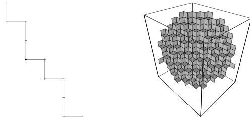
S:={[x, i∗] : x∈Zd,1≤i≤dsuch thatx∈P≥0 and x−ei∈P<0}. Following [6] we call the elements ofS unit tips. The subset ofS with zero translates is especially needed in what follows. Thus we setS0 :={[0, i∗] :
i∈ A} ⊂S. S0consists of three faces of the unit cube located at the origin.
Figure 3. The stepped surfaces associated to the Fibonacci (left) and the Tribonacci (right) substitution.
Letσ be an unimodular Pisot substitution and{Xi}i∈A its atomic sur-faces. It is conjectured that the collection
(2.8) I:={π(x) +Xi : [x, i∗]∈S}
tiles the hyperplaneP(cf. for instance [25]). Up to now, it has been shown that for unimodular Pisot substitutions this is equivalent to the so-called super coincidence condition (cf. [7, 25]; we will give the exact definition in Definition 4.1 below). This condition is conjectured to hold at least for each unimodular Pisot substitution. However, up to now it has been proved only for the case of Pisot substitutions with two letters (cf. Barge and Diamond [7]) as well as for some classes of substitutions with more letters. If this condition does not hold then overlaps occur.
3. Definition of the contact graph
3.1. Geometric realization of substitutions. With help of the prefix-suffix automaton we are in a position to define the one dimensional geo-metric realizationE1(σ) ofσ (cf. [6] or [20, Chapter 8]).
E1(σ)[y, j] :=E0(σ)y− [
(p,i,s),i
i−−−→(p,i,s) j
[f(s), i].
The union is extended over all incoming edges ofj ∈ A in the automaton Γσ. Note thatE1n(σ)[0, i] (i∈ A,n∈N) is a broken line that approximates
the direction of the eigenvector u. Furthermore, we need thedual of this map, namely
E1∗(σ)[x, i∗] :=E0(σ)−1x+
[
(p,i,s),j
i−−−→(p,i,s) j
[E0(σ)−1f(s), j∗].
Here the union is extended over all outgoing edges ofi∈ Ain the automaton Γσ. Note that E1∗(σ)[x, i∗] is the union of all [y, j∗] for which [x, i] occurs
inE1(σ)[y, j], i.e.
(3.1) [y, j∗]∈E1∗(σ)[x, i∗] ⇐⇒ [x, i]∈E1(σ)[y, j].
In the Fibonacci case we have
E1∗(σ)[x,1∗] =E(σ)−1x+ ([e1−e2,1∗]∪[0,2∗]),
In the Tribonacci case one computes
E∗1(σ)[0,1∗] =E(σ)−1x+ ([e1−e3,1∗]∪[e2−e3,2∗]∪[0,3∗]),
E∗1(σ)[0,2∗] =E(σ)−1x+ [0,1∗], E∗1(σ)[0,3∗] =E(σ)−1x+ [0,2∗].
The dual of the one dimensional geometric realization of σ can be used in order to approximate the atomic surfaces ofσ. To make this clear, set (3.2) Xˆi(n) :=
[
[y,j∗]∈E∗
1(σ)n[0,i∗]
π[y, j∗] =πE1∗(σ)n[0, i∗] (n≥0).
Note that ˆXi(0) = π[0, i∗]. Let n ≥ 1. Using the definition of E1∗(σ) we
easily compute that ˆ
Xi(n) =
[
[y1,j∗1]∈E1∗(σ)[0,i∗]
[
[y,j∗]∈E∗
1(σ)n−1[y1,j1∗]
π[y, j∗]
= [
[y1,j∗1]∈E1∗(σ)[0,i∗]
( ˆXj1(n−1) +πE0(σ)−
(n−1)y 1)
= [
i−−−→(p,i,s) j1
( ˆXj1(n−1) +πE0(σ)−nf(s)).
Multiplying by E0(σ)n and setting
(3.3) Xi(n) =E0(σ)nXˆi(n)
we obtain
Xi(n) =
[
i−−−→(p,i,s) j1
(E0(σ)Xj1(n−1) +πf(s)).
This means that if we putXj1(n−1) in the left hand side of the set equation
(2.5) we obtainXi(n). By the general theory of graph directed systems (cf.
for instance [18, Chapter 3] or [28]) this implies that
(3.4) lim
n→∞Xi(n) =Xi and nlim→∞
[
i∈A
Xi(n) =X
in Hausdorff metric. Thus E1∗(σ) can be used to approximate the atomic surfaces in the sense of the Hausdorff metric.
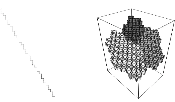
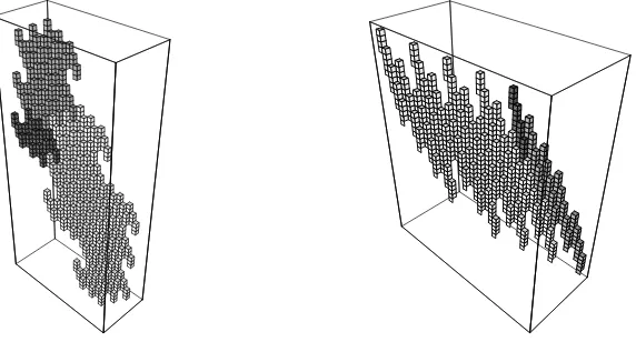
In Figure 4 we see E1∗(σ)8[0, i∗] (i ∈ {1,2}) for the Fibonacci as well asE1∗(σ)10[0, i∗] (i∈ {1,2,3}) for the Tribonacci substitution. In the first case, the approximation consists of unit line segments, in the second case it consists of unit squares.
Figure 4. Approximation of the atomic surfaces with help ofE1∗(σ) for the Fibonacci (left) and the Tribonacci (right) substitution.
Proposition 3.1. Let w= (wℓ)ℓ∈N∈Ωbe a one sided periodic point of σ. Then
Xi=−{πf(w1. . . wk) : k≥0, wk=i} (i∈ A) and X=−{πf(w1. . . wk) : k≥0}.
Proof. We prove the assertion only for X. For Xi everything runs along similar lines. From the set equation (2.5) we see that changing σ to σk
withk≥1 does not change the Rauzy fractalsXi and X. Thus, since σ is
primitive, we may assume w.l.o.g. thatE0(σ) is a positive matrix and that
(after possible rearrangement ofA) w= (wℓ)ℓ∈N = limn→∞σn(1) is a one sided fix point ofσ starting with 1. By (3.4) we know that
X = lim
n→∞π
[
i∈A
E0(σ)nE1∗(σ)n[0, i∗].
Using the duality between E1(σ) and E1∗(σ) we obtain
X=− lim
n→∞π
[
j∈A
Now we have lim
n→∞πE1(σ)
n[0,1] = lim n→∞π
[
(p,i,s)
i−−−→(p,i,s) 1
E1(σ)n−1[−f(s), i]
= lim
n→∞π
[
(p,i,s)
i−−−→(p,i,s) 1
(−E0(σ)n−1f(s) +E1(σ)n−1[0, i])
= lim
n→∞π
[
j∈A
E1(σ)n−1[0, j]
where the last equality follows from the fact thatE0(σ) is a positive matrix
which is a contraction onP. Thus
(3.5) X=− lim
n→∞πE1(σ)
n[0,1].
This is still valid if we take only the limit of the vertices of the broken line
E1(σ)n[0,1]. These vertices are exactly the points of the shapef(w1. . . wk)
(k≥0). Thus we may rewrite (3.5) as
X=−{πf(w1. . . wk) : k≥0}
This proves the result.
3.2. A sequence of sets related to the contact graph. Now we are in a position to construct certain sets, which lead to a generalization of the contact graph, which is well known for lattice tilings (cf. for instance [22, 37]), to atomic surfaces. We will use the above mentioned approxima-tion property in order to approximate the boundary of the setsXi by the
boundary of the setsXi(n) defined in (3.3). We start with the description
of∂Xi(0).
We easily see that
I0 :={π(x) +π[0, i∗] : [x, i∗]∈S}
is a tiling ofP in the sense that it coversPwith overlaps of zero measure. In [25, Theorem 2.5] (see also Arnoux-Ito [6]) it is shown that E1∗(σ) is a so-called “tiling-substitution” which means that
(3.6) In:={π(x) +Xi(n) : [x, i∗]∈S}
also forms a tiling of Pfor each n∈N. First considerI0. Because I0 is a tiling of P, the boundary of a tile π[0, i∗] (i∈ A) is a union of sets of the form
π([0, i∗]∩[y, j∗]) (π[y, j∗]∈ I0, [y, j∗]6= [0, i∗]).
is a uniformly discrete subset of P. Moreover, since the tiles are (d− 1)-dimensional prisms, we only have to take intersections with tiles which pair a (d−2)-dimensional face with π[0, i∗]. Let Ui be the set of all unit tips, which pair at least (d−2)-dimensional faces with the unit tip [0, i∗] (i∈ A), i.e.
Ui :={[y, j∗]∈S : Ld−2([y, j∗]∩[0, i∗])>0}
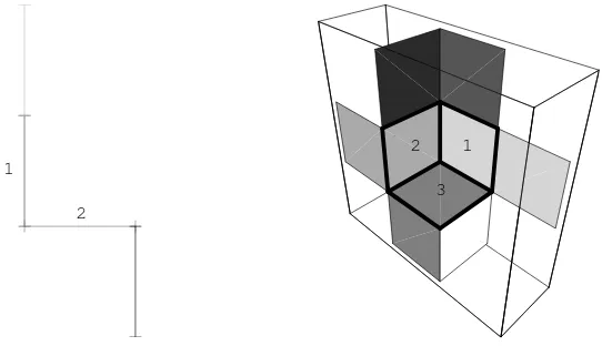
(Lk is the k-dimensional Lebesgue measure). In Figure 5 we depict the
elements ofU1∪U2for the Fibonacci as well as the elements ofU1∪U2∪U3
for the Tribonacci substitution. In the case of the Fibonacci substitution the boundary ofπ[0, i∗] (i∈ {1,2}) consists of exactly two points (the end points of the line segment [0, i∗]). In the Tribonacci case the boundaries of the “central” unit tips [0, i∗] (i ∈ {1,2,3}) are indicated by boldface lines. These boundaries are unions of line segments which come from the intersection of two unit tips.
1
2
3 1 2
Figure 5. The unit tips which pair at least (d − 2)-dimensional faces with the “central” unit tips [0, i∗] for the Fibonacci (left) and the Tribonacci (right) substitution. The set [0, i∗] is indicated byi.
Let
(3.7) Q:={([x, i∗],[y, j∗]) : [x, i∗],[y, j∗]∈S withx= 0 ory= 0}.
Throughout the present paper we identify the elements ([x, i∗],[y, j∗]) and ([y, j∗],[x, i∗]). We will say that an element of Q is written in canonical orderif it is written in the form
(
([0, i∗1],[z, i∗2]) ifz6= 0,
In order to keep the analogy to the contact matrix of lattice tilings (cf. [22]) we set
R0 := [
i∈A
{([0, i∗],[y, j∗])∈ Q : [y, j∗]∈Ui}.
Note that R0 is the set of all pairs which correspond to non-empty
inter-sections of the formπ([0, i∗]∩[y, j∗]). Thus (3.8) ∂π[0, i∗] = [
([0,i∗][y,j∗])∈R0 [0,i∗]6=[y,j∗]
π([0, i∗]∩[y, j∗]) (i∈ A).
Looking at Figure 5 again, we see that for the Fibonacci substitution we have #R0 = 5 (two line segments plus three end points), while in the
Tribonacci case we have #R0 = 12 (3 surfaces corresponding to the
ele-ments ([0, i∗],[0, i∗]); furthermore, the boundary consists of 9 different line segments).
Thus R0 contains full information on the boundary of the sets Xi(0) =
π[0, i∗]. We now want to set up a sequence of sets Rn which contains full
information on the boundaries of the sets Xi(n). Before we do this in full generality, we want to provide the construction of R1 starting from R0 in
full detail. To this end we defineϕ:S×S→ Q by (3.9) ϕ([x1, i∗1],[x2, i∗2]) :=
(
([0, i∗1],[x2−x1, i∗2]) if (x1−x2)·v <0,
([0, i∗2],[x1−x2, i1∗]) if (x1−x2)·v≥0.
It remains to check thatϕmaps toQ. If the first alternative in the definition of ϕ holds it suffices to show that [x2−x1, i∗2] ∈ S. For this alternative (x2−x1)·v >0 holds. Furthermore, we have
(x2−x1−ei2)·v= (x2−ei2)·v−x1·v <−x1·v≤0
because [x1, i∗1],[x2, i∗2]∈S. This proves that [x2−x1, i∗2]∈S. The second
alternative is treated likewise. We set
R1 :=R0∪
n
ϕ([x1, i∗1],[x2, i∗2])∈ Q : ∃([0, j1∗],[y, j2∗])∈R0
with [x1, i1]∈E1(σ)[0, j1] and [x2, i2]∈E1(σ)[y, j2]o.
Lemma 3.2. Let [x1, i∗1] and [x2, i∗2] be elements of S. Then π([x1, i∗1]∩
[x2, i∗2])forms a (d−2)-dimensional face if and only ifϕ([x1, i∗1],[x2, i∗2])∈
R0.
Proof. This is an easy consequence of the definitions of ϕand R0.
Proposition 3.3. The boundary of Xi(1) is given by
(3.10) ∂Xi(1) =
[
([0,i∗][y,j∗])∈R
1
[0,i∗]6=[y,j∗]
(Xi(1)∩(Xj(1) +π(y))) (i∈ A).
Proof. As mentioned above, I1 forms a tiling of P. Thus the boundary of
the setXi1(1) (i1 ∈ A) consists of sets of the shapeXi1(1)∩(Xi2(1)+π(x)). SinceXi1(1) is a finite union of (d−1)-dimensional prisms, it suffices to take
into account only intersections that contain at least one (d−2)-dimensional face. Because
Xi1(1) =
[
[y,j∗]∈E∗
1(σ)[0,i∗]
E0(σ)(Xj(0) +π(y))
the intersectionXi1(1)∩(Xi2(1) +π(x)) contains a (d−2)-dimensional face
if and only if there exist
[y1, j1∗]∈E1∗(σ)[0, i∗1] and [y2, j2∗]∈E1∗(σ)[x, i∗2]
such thatπ([y1, j1∗]∩[y2, j2∗]) forms a (d−2)-dimensional face, i.e., in view
of Lemma 3.2, if and only if (3.11)
[y1, j∗1]∈E1∗(σ)[0, i1∗], [y2, j2∗]∈E1∗(σ)[x, i∗2] and ϕ([y1, j1∗],[y2, j2∗])∈R0.
Using the duality relation (3.1) betweenE1(σ) andE1∗(σ) we see that (3.11)
is equivalent to the existence of [y1, j1∗],[y2, j2∗]∈S such that
(3.12)
[0, i1]∈E1(σ)[y1, j1], [x, i2]∈E1(σ)[y2, j2] and ϕ([y1, j1∗],[y2, j2∗])∈R0.
We have to distinguish two cases according to the two cases in the defi-nition of ϕin (3.9).
• Suppose first thatϕ([y1, j1∗],[y2, j2∗]) = ([0, j1∗],[y2−y1, j2∗]) holds and sety =y2−y1. Translating the first two statements of (3.12) by the
vector−E0(σ)y1 yields
[−E0(σ)y1, i1]∈E1(σ)[0, j1], [x−E0(σ)y1, i2]∈E1(σ)[y, j2] and
([0, j1∗],[y, j2∗])∈R0.
Because [x, i∗2] is a unit tip we have
ϕ([−E0(σ)y1, i∗1],[x−E0(σ)y1, i∗2]) = ([0, i∗1],[x, i∗2]).
• Now suppose thatϕ([y1, j1∗],[y2, j2∗]) = ([0, j2∗],[y1−y2, j1∗]) holds and
sety =y1−y2. Translating the first two statements of (3.12) by the
vector−E0(σ)y2 yields
and
([0, j2∗],[y, j1∗])∈R0.
Because [x, i∗2] is a unit tip we have
ϕ([−E0(σ)y2, i∗1],[x−E0(σ)y2, i∗2]) = ([0, i∗1],[x, i∗2]).
In both cases (3.12) implies the existence of [x1,˜i∗1],[x2,˜i∗2] ∈Zd× A and
([0, j1∗],[y, j2∗])∈R0 such that
([0, i∗1],[x, i∗2]) =ϕ([x1,˜i∗1],[x2,˜i∗2]),
[x1,˜i1]∈E1(σ)[0, j1] and [x2,˜i2]∈E1(σ)[y, j2].
By the definition ofR1 this implies that ([0, i∗1],[x, i∗2])∈R1.
Summing up we have shown that Xi1(1)∩(Xi2(1) +π(x)) contains a
(d−2)-dimensional face only if ([0, i∗1],[x, i∗2])∈R1. Hence, we may write
the boundary ofXi(1) as
∂Xi(1) = [
([0,i∗
1][x,i∗2])∈R1
[0,i∗
1]6=[x,i∗2]
(Xii(1)∩(Xi2(1) +π(x))) (i∈ A)
and the result is proved.
The fact that we addR0 in the definition ofR1 has technical reasons. It
ensures that the sequence {Rn}n≥0 defined below is increasing.
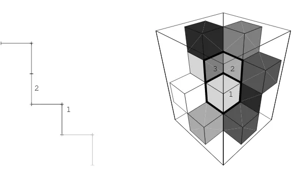
In Figure 6 the sets E1∗(σ)[y, j∗] for which ([0, i∗][y, j∗]) ∈ R1 are
de-picted. In the Fibonacci case we have ˆ
X1(1) =πE1∗(σ)[0,1∗] =π([e1−e2,1∗]∪[0,2∗]),
ˆ
X2(1) =πE1∗(σ)[0,2∗] =π[0,1∗].
In the Tribonacci case one computes ˆ
X1(1) =πE1∗(σ)[0,1∗] =π([e1−e3,1∗]∪[e2−e3,2∗]∪[0,3∗]),
ˆ
X2(1) =πE1∗(σ)[0,2∗] =π[0,1∗],
ˆ
X3(1) =πE1∗(σ)[0,3∗] =π[0,2∗].
1 2
1 2 3
Figure 6. Illustration of the setR1 for the Fibonacci (left)
and the Tribonacci (right) substitution. The setE1∗(σ)[0, i∗] is indicated byi.
Now we turn to the general case. We constructRn+1 starting fromRnin
the same way as we constructedR1 starting fromR0. Thus starting with
R0 we define the sequence {Rn}n∈N by a recurrence relation. This is done by the following set function. Let 2Q be the set of all subsets ofQ. Then
Ψ : 2Q → 2Q,
M 7→ M∪nϕ([x1, i∗1],[x2, i∗2])∈ Q : ∃([0, j1∗],[y, j2∗])∈M
with [x1, i1]∈E1(σ)[0, j1] and [x2, i2]∈E1(σ)[y, j2]
o .
Now suppose thatR0, . . . , Rnare already defined. Then Rn+1 is defined in
terms ofRn by
(3.13) Rn+1 := Ψ(Rn).
In Lemma 4.2 we will show that the setsRnadmit a generalization of (3.10)
for the boundaries ∂Xi(n) (n ≥ 1). The following lemma shows that the sequence {Rn}n∈N is ultimately constant.
Lemma 3.4. Let σ be a unimodular Pisot substitution and attach to it the sequence of sets {Rn} defined in (3.13). Then there exists an effectively
computable integer N ∈N such that RN =Rn for all n≥N. Thus we set
R:=RN. R contains only finitely many elements.
Proof. Let ΛC:= diag(λ1, . . . , λd) and letT be a regular matrix satisfying E0(σ) := T−1ΛCT. Let n ≥ 1 be arbitrary. By the definition of Rn an
element ([0, i∗1],[r, i∗2])∈Rn satisfies r=±E0(σ)nx+
n−1
X
k=0
where ([0, j∗1],[x, j2∗])∈R0 andsk andtk are suffixes of strings of the shape σ(j) for certain j ∈ A. Setting rk = (rk(1), . . . , rk(d)) := T(f(sk)−f(tk)) (0≤k≤n−1) and q= (q(1), . . . , q(d)) :=T xthis yields
T r =±ΛnCq+
n−1
X
k=0
ΛkCrk
= ±λn1q(1)+
n−1
X
k=0
λk1r(1)k , . . . ,±λndq(d)+
n−1
X
k=0
λkdr(kd) !
.
The first coordinate of T r is bounded by a constant L1 depending only
on the choice of T because [r, j∗] is a unit tip. The other coordinates are bounded by a constantL2 because rk and q can attain only finitely many
values and|λi|<1 for 2≤i≤d.
In other words, the elements ([0, i∗],[r, j∗])∈Rn satisfy
||T r||∞≤L
for some absolute constant L. This implies that the number of elements in Rn is uniformly bounded in n. Since Rn ⊆ Rn+1 it follows that the
sequence {Rn}is ultimately constant.
Corollary 3.5. Let R0⊆M ⊆R. Then Ψ(M) =M implies thatM =R. Proof. Note that M1 ⊆ M2 implies that Ψ(M1) ⊆Ψ(M2). Select N such
thatRN = ΨN(R0) =R. Suppose that Ψ(M) =M. Then
R= ΨN(R0)⊆ΨN(M) =M ⊆R
and we are done.
3.3. The contact graph. Before we give the exact definition of the con-tact graph we recall the definition of the adjacency matrix AG = (aij) of
a finite directed graph G (cf. [27, Definition 2.2.3]). Let V = {1, . . . , q} be the set of states ofG. Then AG is aq×q matrix with aij equal to the
number of edges inGleading formitoj. The order of the states will play no role in our context. In particular, changing the order of the states ofG
does not change the eigenvalues ofAG.
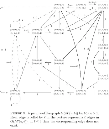
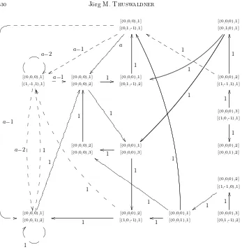
Definition 3.6. Let σ be a unimodular Pisot substitution and let Q be defined as in (3.7). If M ⊂ Q then the contact graph G(M) of M is given in the following way. The states ofG(M) are the elements of M. Each of the states is an initial state. Furthermore, there exists an edge
(3.14)
([0, i∗1],[x, i∗2])−−→P|Q ([0, j1∗],[y, j2∗]) (states written in canonical order) withP := (p1, i1, s1) and Q:= (p2, i2, s2) in G(M) if
and
(3.15) σ(jk) = (pk, ik, sk)∈ P (1≤k≤2) or
σ(j3−k) = (pk, ik, sk)∈ P (1≤k≤2).
If the first alternative in (3.15) holds, the corresponding edge is said to be of type 1, if the second alternative holds, it is of type 2. If both alternatives hold, we also say that the edge is of type 1.
The adjacency matrix of G(M) is called the contact matrix ofM. IfM =R thenC:=G(R) is called the contact graph ofσ. Its adjacency matrix is called the contact matrix of σ.
Obviously, all the graphs G(M) are subgraphs of the graph G(Q). Remark 3.7. Note that the two alternatives we have for the edges corre-spond to the two alternatives in the definition of ϕ. In fact, inserting the definition ofΨ we see that the edge (3.14)exists if either
x=E0(σ)y+f(s1)−f(s2) such that σ(jk) = (pk, ik, sk)∈ P
(1≤k≤2)or
x=−E0(σ)y−f(s2) +f(s1) such that σ(j3−k) = (pk, ik, sk)∈ P
(1 ≤ k ≤ 2). Indeed, ([0, i∗1],[x, i2∗]) ∈ Ψ{([0, j1∗],[y, j2∗])} implies that ([0, i∗1],[x, i∗2]) = ϕ([−f(˜s1),˜i∗1],[E0(σ)y−f(˜s2),˜i∗2]) with σ(jk) = ˜pk˜iks˜k
(1≤k≤2). According to the definition of ϕ this implies that ([0, i∗1],[x, i∗2]) =
(
[0,˜i∗1],[E0(σ)y−f(˜s2) +f(˜s1),˜i∗2] or
[0,˜i∗2],[−E0(σ)y+f(˜s2)−f(˜s1),˜i∗1].
The desired formulas are obtained by setting(pk, ik, sk) = (˜pk,˜ik,s˜k) in the
first case and(pk, ik, sk) = (˜p3−k,˜i3−k,˜s3−k)in the second case (1≤k≤2). Both alternatives (type 1 and type 2) can hold for an edge simultaneously only if σ(j1) = σ(j2) and, hence, (p1, i1, s1) = (p2, i2, s2). This implies
j1 = j2. Thus we must have x =E0(σ)y and x = −E0(σ)y. Since E0(σ) is a regular matrix we must therefore have x = y = 0. Summing up we conclude that both alternatives can hold simultaneously only for an edge of the shape
([0, i∗],[0, i∗])−−→P|P ([0, j∗],[0, j∗]).
Throughout the paper we will always assume that the states of the oc-curring graphs are written in canonical order. It is easy to see that the edge
(3.16) ([0, i∗],[0, i∗])−−→P|Q ([0, j∗1],[y, j∗2]) exists if and only if
exists. Thus we will always identify these two edges.
Definition 3.6 generalizes the graphG(R), which was defined by Scheicher and Thuswaldner [36, 37] for lattice tilings. The contact matrix for lattice tilings first appears in Gr¨ochenig and Haas [22].
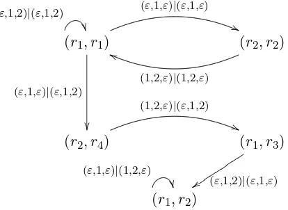
For the Fibonacci substitution it is fairly easy to calculate the contact graph. In fact, we have R0 = R1 = R. Thus R has 5 elements. From
Figure 5 we easily see that
R={(r1, r1),(r1, r2),(r1, r3),(r2, r2),(r2, r4)}
with r1 = [0,1∗], r2 = [0,2∗], r3 = [(0,1),1∗] and r4 = [(1,−1),1∗]. If we
draw the edges between these states according to Definition 3.6 we arrive at the graph depicted in Figure 7 (ε denotes the empty word). Observe that it contains a copy of the corresponding prefix-suffix automaton.
(r1, r1)
(ε,1,2)|(ε,1,2)
(ε,1,ε)|(ε,1,ε)
(
(
(ε,1,ε)|(ε,1,2)
(r2, r2)
(1,2,ε)|(1,2,ε)
h
h
(r2, r4)
(1,2,ε)|(ε,1,2)
(
(
(r1, r3) (ε,1,2)|(ε,1,ε)
y
y
tttt tttt
t
(r1, r2) (ε,1,ε)|(1,2,ε)
Figure 7. The contact graph of the Fibonacci substitution.
The contact graph of the Tribonacci substitution will be constructed later. It is described in Theorem 6.4.
Lemma 3.8. Let σ be a unimodular Pisot substitution and let H be a subgraph ofG(Q). If from each state([0, i∗1],[x, i∗2])of H there leads a walk to a state ([0, j1∗],[y, j2∗])∈R0 then H⊂ C =G(R).
Proof. By definition,Rcontains all elements ([0, i∗1],[x, i∗2])∈ Qfrom which there leads a walk to a state of the shape ([0, j1∗],[y, j2∗])∈R0inG(Q). Since
H⊆G(Q) we are done.
4. On the boundary of a tile
of the tilings In defined in (3.6) for n → ∞yields a tiling. Let Xi(n) be
defined as in (3.3). SinceXi(n)→Xi this is tantamount to saying thatI
in (2.8) tiles P. As mentioned in the introduction this is true only if the so-called super coincidence condition holds.
Definition 4.1 (cf. [7, 25]). Let[x, i]and[y, j]with x, y∈Zdand i, j∈ A be given. We say that[x, i]and [y, j]have strong coincidence if there exists ann∈Nsuch thatE1(σ)n[x, i]∩E1(σ)n[y, j]have at least one line segment in common.
Let π′ be the projection ofRd to u along P. We say that [x, i] and [y, j] have the same height if
int(π′[x, i])∩int(π′[y, j])6=∅.
Furthermore, σ satisfies the super coincidence condition if [x, i] and [y, j] have strong coincidence whenever they have the same height.
If this condition holds for σ then [25, Theorem 1.3] yields that I tiles P. Together with [25, Theorem 3.3] this implies that ( ˆXi(n) is defined in (3.2))
(4.1) lim
n→∞E0(σ)
n∂Xˆ
i(n) =∂Xi (i∈ A)
in Hausdorff metric (cf. also [20, Chapter 8] and [6]; for the lattice tile analogue of these results we refer to Vince [43, Theorem 4.2]). Setting
ˆ
X(n) :=Si∈AXˆi(n) an analogous identity holds for ∂X.
4.1. The boundaries of the approximations of Xi. For fixed n the set ˆXi(n) in (3.2) is the union of (d−1)-dimensional prisms of the shape π[x, i∗]. Its boundary is a union of (d−2)-dimensional prisms of the shape (4.2) π[x1, i∗1]∩π[x2, i∗2].
LetQ be defined as in (3.7). For ([0, i∗1],[x, i∗2])∈ Qlet
(4.3) B(([0, i∗1],[x, i∗2]), n) := ˆXi1(n)∩( ˆXi2(n) +E0(σ)−nπ(x)).
If [0, i∗1]6= [x, i∗2] then B(([0, i∗1],[x, i∗2]), n) consists of a union of prisms of the shape (4.2). The number of these prisms will be denoted by
Π (B(([0, i∗1],[x, i∗2]), n)).
Lemma 4.2. Let σ be a unimodular Pisot substitution. If [0, i∗1]6= [x, i∗2] then forn≥0 we have
Π(B(([0, i∗1],[x, i∗2]), n))>0 =⇒ ([0, i∗1],[x, i∗2])∈Rn.
If n is large enough such thatRn=R then this becomes
This implies that
Proof. We use induction on nin order to prove the lemma. For n= 0 the result is true by (3.8). Now suppose that it is true for n−1. Then we get
Inserting the definition ofE1∗(σ) in the first union yields
Changing the order of the unions and inserting the definition of ˆXℓ(n−1) forℓ=j1 and j2 yields that this is equal to
[
i1
(p1,i1,s1) −−−−−−→j1
[
i2
(p2,i2,s2) −−−−−−→j2
ˆ
Xj1(n−1) +πE0(σ)−
nf(s 1)
∩Xˆj2(n−1) +πE0(σ)−
n(f(s 2) +x)
= [
i1
(p1,i1,s1) −−−−−−→j1
[
i2
(p2,i2,s2) −−−−−−→j2
[E0(σ)−1(f(s2)−f(s1)+x),j2∗]∈S
B ([0, j1∗],[E0(σ)−1(f(s2)−f(s1) +x), j2∗]), n−1
+ πE0(σ)−nf(s1)
∪ [
i1
(p1,i1,s1) −−−−−−→j1
[
i2
(p2,i2,s2) −−−−−−→j2
[−E0(σ)−1(f(s2)−f(s1)+x),j1∗]∈S
B ([0, j2∗],[−E0(σ)−1(f(s2)−f(s1) +x), j1∗]), n−1
+πE0(σ)−n(f(s2) +x)
.
The fact that we have to split up the double unions in two parts comes from the definition ofϕ. Note that one of the quantities [E0(σ)−1(f(s2)−
f(s1) +x), j2∗] and [−E0(σ)−1(f(s2)−f(s1) +x), j1∗] is always contained
by definition. Summing up we proved that Π(B(([0, i∗1],[x, i∗2]), n))
= Π [
i1
(p1,i1,s1) −−−−−−→j1
[
i2
(p2,i2,s2) −−−−−−→j2
[E0(σ)−1(f(s2)−f(s1)+x),j2∗]∈S
B ([0, j1∗],[E0(σ)−1(f(s2)−f(s1) +x), j2∗]), n−1
+πE0(σ)−nf(s1)
∪ [
i1
(p1,i1,s1) −−−−−−→j1
[
i2
(p2,i2,s2) −−−−−−→j2
[−E0(σ)−1(f(s2)−f(s1)+x),j1∗]∈S
B ([0, j2∗],[−E0(σ)−1(f(s2)−f(s1) +x), j1∗]), n−1
+
πE0(σ)−n(f(s2) +x)
! .
By the induction hypothesis this is greater than zero if and only if at least one of the elements
([0, j1∗],[E0(σ)−1(f(s2)−f(s1) +x), j2∗])
or
([0, j2∗],[−E0(σ)−1(f(s2)−f(s1) +x), j1∗])
is contained in Rn−1. If this is the case then by the definition of Rn in
terms ofRn−1 we have ([0, i∗1],[x, i∗2])∈Rnand we are done.
4.2. A set equation for the boundaries of Xi. In the remaining part
of the paper we will always assume that σ satisfies the super coincidence condition. We are now in a position to give a description of the boundaries ofXi (i∈ A) as a graph directed system.
Letǫ: ([0, i∗1],[x, i2∗])−−−−−−−−−−−−→(p1,i1,s1)|(p2,i2,s2) ([0, j1∗],[y, j2∗]) be an edge inC(the states are written in canonical order) and set
F(ǫ) :=
(
f(s1) ifǫis of type 1,
f(s2) +x ifǫis of type 2.
Remark 3.7 we have x = 0 and s1 = s2 in this case. An easy calculation
shows thatF(ǫ) is the same for the identified edges (3.16) and (3.17). We define the non-empty compact setsC(v)⊂P(v∈R) by the following graph directed system:
(4.4) C(v1) =
[
ǫ:v1→v2
E0(σ)C(v2) +πF(ǫ).
The union is extended over all outgoing edges ofv1 in the contact graphC.
In particular,C(v) is empty if the state v has no outgoing edges.
Theorem 4.3. Let σ be a unimodular Pisot substitution which satisfies the super coincidence condition and let X and {Xi}i∈A be the associated atomic surfaces. The boundaries of X andXi (i∈ A) can be characterized
as follows.
∂X = [
([0,i∗],[y,j∗])∈R
y6=0
C(([0, i∗],[y, j∗])),
(4.5)
∂Xi=
[
([0,i∗],[y,j∗])∈R
i fixed,[0,i∗]6=[y,j∗]
C(([0, i∗],[y, j∗])) (i∈ A),
(4.6)
where C(v) (v∈R) is uniquely defined by the graph directed system (4.4). Remark 4.4. Note that equation (4.4) is related to the dual map E∗2(σ) of the two dimensional realization E2(σ) of σ in Sano et al. [35]. With help of this dual map one also gets a parametrization of the boundary ofXi
(cf. [35, Proposition 3.1]). This technique was used in Ito-Kimura [24] to determine the Hausdorff dimension of the boundary of the classical Rauzy fractal.
Proof. Let N be large enough such that RN = R. Then by the same
reasoning as in the proof of Lemma 4.2 we get
B(v1, n) =
[
ǫ:v1→v2
B(v2, n−1) +πE0(σ)−nF(ǫ).
ThusE0(σ)nB(v, n) converges toC(v) forn→ ∞in Hausdorff metric (cf.
[18, Theorem 2.6 and Chapter 3]), i.e.
(4.7) C(v) = lim
n→∞E0(σ)
nB(v, n)
holds for eachv∈R. Since
∂Xˆ(n) = [
([0,i∗
1],[x,i∗2])∈Q
x6=0
Lemma 4.2 implies that
(4.8) ∂Xˆ(n) = [
([0,i∗
1],[x,i∗2])∈R
x6=0
B(([0, i1],[x, i∗2]), n).
Note that ifAn→A,Bn→B andAn∪Bn→C in Hausdorff metric then
C =A∪B. Thus multiplying by E0(σ)n and taking limits in (4.8), (4.1)
yields (4.6). (4.5) is shown analogously.
Forv ∈Rlet C(v) be defined as in (4.4). Using (4.7), (4.3) and (4.1) we see that
C(([0, i∗],[0, i∗])) = lim
n→∞E0(σ)
nB([0, i∗],[0, i∗], n) = lim
n→∞E0(σ)
nXˆ i(n)
=Xi.
Thus the state ([0, i∗],[0, i∗]) inC corresponds to the set Xi. Suppose that
there exists an edge ([0, i∗1],[x, i∗2]) → ([0, j∗],[0, j∗]) in C. Then, by (4.4) the set C(([0, i∗1],[x, i∗2])) contains a shrinked copy of Xj. Thus the set C(([0, i∗1],[x, i∗2])) has inner points because Xj has inner points by Propo-sition 2.3. But since by assumption there are no overlaps in the tiling I this implies that i1 = i2 and x = 0 and, hence, C(([0, i∗1],[x, i∗2])) = Xi1. Thus we may omit the states ([0, i∗],[0, i∗]) from C without affecting (4.4) for those setsC(v) which are subsets of the boundary of one of the setsXi.
From the resulting subgraph we may successively omit all states having no outgoing edge because the sets C(v) corresponding to these states v are empty. Thus we loose nothing by omitting these states. This motivates the following definition.
Definition 4.5. Let Cbe the contact graph. Delete the states([0, i∗],[0, i∗]) fromC and from the resulting subgraph successively delete all states having no outgoing edges. The boundary graph emerging from this process will be denoted by C∂.
In the sequel we will need the following definitions (cf. for instance [27, p. 37]). LetGbe a directed graph. We call a statevofGastranding state if no edges start atv or no edges terminate at v. Gis called essentialif it contains no stranding states. The graph emerging fromGby removing all stranding states is called theessential partof G.
LetC∂′ be the essential part of C∂ (i.e. remove all states ofC∂ having no
incoming edges) and let V ∈ C∂ be an arbitrary state. Since each state of
C∂ has outgoing edges we conclude that each walk starting atV arrives at
a stateV′∈ C′
4.3. Using prefixes instead of suffixes. Let σ be a unimodular Pisot substitution. All the definitions and results of this paper can be estab-lished also by working with prefixes instead of suffixes. In this case the set equation in (2.5) for the atomic surfacesXi′ associated to σ reads
Xi′ = [
(p,i,s),j
i−−−→(p,i,s) j
E0(σ)Xj′ −πf(p)
where
Xi′ =Xi+π(ei) (i∈ A)
(cf. [6, Lemma 8]). Moreover, the following slight modifications are needed (cf. [6]). Firstly, we have to set [x, i] :={x+θei : θ∈[0,1]} and
[x, i∗] :={x+ei+θ1e1+. . .+θi−1ei−1+θi+1ei+1+. . .+θded) : θi∈[0,1]}.
The stepped surfaceS has to be
S :={[x, i∗] : x∈Zd,1≤i≤dsuch thatx∈P<0 and x+ei∈P≥0} in the prefix setting, the setS0 is defined byS0:={[−ei, i∗] : i∈ A} ⊂S. The definitions of ϕ and Q have to be changed accordingly. For the one dimensional geometric realizationE1(σ) and its dual E1∗(σ) we have
E1(σ)[y, j] :=E0(σ)y+ [
(p,i,s),i
i−−−→(p,i,s) j
[f(p), i]
and
E1∗(σ)[x, i∗] :=E0(σ)−1x− [
(p,i,s),j
i−−−→(p,i,s) j
[E0(σ)−1f(p), j∗].
These modifications cause that different pairs of unit tips pair (d− 2)-dimensional faces with each other. However, the structure of the resulting contact graph is of course the same because both constructions are equiv-alent.
5. Hausdorff and box counting dimension of the boundary Throughout this section we assume that the super coincidence condition is fulfilled for the substitutions under discussion. By Theorem 4.3 we know that ∂X is a graph directed self-affine set directed by C∂. We will now
determine the box counting dimension of ∂X and ∂Xi (i ∈ A). If ∂X
5.1. Preparation: construction of covers. We will use the notation
WL(V, V′) for all walks from a state V to a stateV′ of length L inC∂ and WL(V) for all walks in C∂ starting at V. The set of all walks of length L
inC∂ will be denoted by WL.
Let
(5.1) ǫ: ([0, i∗1],[x, i2∗])−−−−−−−−−−−−→(p1,i1,s1)|(p2,i2,s2) ([0, j∗1],[y, j∗2]) (states written in canonical order) be an edge inC∂ and define
χǫ: P → P,
t 7→ E0(σ)t+πF(ǫ).
More generally, let
(5.2) w: VL−−−−→PL|QL VL−1 −−−−−−−→ · · ·PL−1|QL−1 −−−−→P1|Q1 V0
be a walk inWL and setVℓ := ([0, iℓ∗],[xℓ, jℓ∗]) (written in canonical order). Denote the edgeVℓ−−−→Pℓ|Qℓ Vℓ−1 by ǫℓ. Then set
χw : P → P,
t 7→ χǫL◦ · · · ◦χǫ1(t).
Note that the functionsχw are contractions sinceE0(σ) is a contraction on P.
We associate two walks of the prefix-suffix automaton Γσ (see
Defini-tion 2.2) to the walkw in (5.2) in the following way. First we set
(p1, i1, s1) :=
(
P1 ifǫ1 is of type 1, Q1 ifǫ1 is of type 2,
(q1, j1, t1) :=
(
P1 ifǫ1 is of type 2,
Q1 ifǫ1 is of type 1.
For 2 ≤ℓ≤ L we define (pℓ, iℓ, sℓ) and (qℓ, jℓ, tℓ) iteratively as follows. If
we have defined (pℓ−1, iℓ−1, sℓ−1) :=Pℓ−1 then
(pℓ, iℓ, sℓ) :=
(
Pℓ ifǫℓ is of type 1, Qℓ ifǫℓ is of type 2,
(qℓ, jℓ, tℓ) :=
(
If, at the contrary, we have defined (pℓ−1, iℓ−1, sℓ−1) :=Qℓ−1 then
(pℓ, iℓ, sℓ) :=
(
Qℓ ifǫℓ is of type 1, Pℓ ifǫℓ is of type 2,
(qℓ, jℓ, tℓ) :=
(
Qℓ ifǫℓ is of type 2, Pℓ ifǫℓ is of type 1.
The reason why we defined these quantities in this way is that according to the definition ofC∂ the sequences (pℓ, iℓ, sℓ)L≥ℓ≥1 and (qℓ, jℓ, tℓ)L≥ℓ≥1 give
rise to walks in Γσ (with L ≥ ℓ ≥ 1 we mean that the walk starts with
(pL, iL, sL) and ends with (p1, i1, s1)).
Lemma 5.1. Let w∈WL be the walk in (5.2)and associate the sequences
(pℓ, iℓ, sℓ)L≥ℓ≥1 and(qℓ, jℓ, tℓ)L≥ℓ≥1 to it as above. If PL= (pL, iL, sL) then
(5.3) x0 =E0(σ)−LxL+
L
X
ℓ=1
E0(σ)−ℓ(f(tℓ)−f(sℓ)),
if PL= (qL, jL, tL) then
(5.4) x0=−E0(σ)−LxL+ L
X
ℓ=1
E0(σ)−ℓ(f(tℓ)−f(sℓ)).
Proof. This can easily be proved by induction on L. If (5.3) holds for a certain L ∈ N we will say for short that A1(L) holds. Similar, if (5.4) is true for a certain L∈Nwe will say that A2(L) holds.
Let Vℓ be defined as above. We start with L = 1. If ǫ1 is of type 1
then P1 = (p1, i1, s1) and Q1 = (q1, j1, t1). Using the definition of C∂ we
get x0 = E0(σ)−1x1+E0(σ)−1(f(t1)−f(s1)). If ǫ1 is of type 2 we have
P1 = (q1, j1, t1) and Q1 = (p1, i1, s1). This yields x0 = −E0(σ)−1x1 +
E0(σ)−1(f(t1)−f(s1)).
Now we turn to the induction step. We will proveA1(L) andA2(L) as-sumingA1(L−1) andA2(L−1): Suppose first thatPL−1 = (pL−1,iL−1,sL−1)
and that A1(L−1) is true. If ǫL is of type 1 then PL = (pL, iL, sL) and QL= (qL, jL, tL). Applying the definition of C∂ this implies that
xL−1 =E0(σ)−1xL+E0(σ)−1(f(tL)−f(sL)).
Inserting this inA1(L−1) provesA1(L) in this case. IfǫLis of type 2 then PL= (qL, jL, tL) and QL= (pL, iL, sL). The proof of A2(L) is done in the same way in this case.
Now assume that PL−1 = (qL−1,jL−1,tL−1) holds and that A2(L−1)
is true. If ǫL is of type 1 then PL = (qL, jL, tL) and QL = (pL, iL, sL).
Applying the definition ofC∂ this implies that
Inserting this inA2(L−1) provesA2(L) in this case. IfǫLis of type 2 then PL= (pL, iL, sL) and QL= (qL, jL, tL). The proof of A1(L) is done in the
same way in this case.
Let ρ > 0 and let B be an arbitrary ball of radius ρ. Iterating (2.5) L
times, multiplying byE0(σ)−Land observing that the setsXj are compact
and have non-empty interior by Proposition 2.3, we see that there is a con-stantcρindependent ofLwhich bounds the number of walks (qℓ, jℓ, tℓ)L≥ℓ≥1
of Γσ having lengthL and satisfying L
X
ℓ=1
E0(σ)−ℓf(tℓ)∈ B.
Lemma 5.2. The number of walks in WL corresponding to a given walk
(pℓ, iℓ, sℓ)L≥ℓ≥1 of Γσ is uniformly bounded inL.
Proof. Let wbe defined as in (5.2). By Lemma 5.1 we have
x0=±E0(σ)−LxL+
follows from the remark preceding this lemma.
Lemma 5.3. Let w∈WL be as in (5.2)and associate (pℓ, iℓ, sℓ)L≥ℓ≥1 and
We proceed with the induction step. Let w′ be the walk emerging from
If ǫL is of type 2, i.e. PL = (qL, jL, tL), then F(ǫL) = f(sL) +xL and the
Proof. Let L be arbitrary, but fixed. We will prove the assertion for
E0(σ)−Lχw(Z) instead of χw(Z). Because E0(σ) is regular, this does not make a difference. In what follows let (pℓ, iℓ, sℓ)L≥ℓ≥1and (qℓ, jℓ, tℓ)L≥ℓ≥1be
walks in Γσ. SinceZ is bounded, the remark preceding Lemma 5.2 assures
that there exists an absolute constantc1such thatZ+πPLℓ=1E0(σ)−ℓf(tℓ)
has non-empty intersection with at mostc1 sets of the shape
Xj +π L
X
ℓ=1
E0(σ)−ℓf(sℓ).
From the same fact it follows that there even exists an absolute constant
c2 such that Z+πPLℓ=1E0(σ)−ℓf(tℓ) has non-empty intersection with at
By Lemma 5.2 there is an absolute constantc3which bounds the number of
w∈WLcorresponding to a given walk (pℓ, iℓ, sℓ)L≥ℓ≥1 of Γσ. Furthermore,
Let Λ and TP be defined as in Subsection 2.3. The dimension
calcula-tions are done for the sets C(v) with v ∈ C∂ defined in (4.4). Since it is
more convenient to work with affine transformations whose linear part is in diagonal form we work with the sets
D(v) :=TPC(v).
From (4.4) we immediately get that
D(v1) =
[
ǫ:v1→v2
ΛD(v2) +TPπF(ǫ).
Letǫbe an edge in C∂ as in (5.1). Then we set ψǫ(t) := Λt+TPπF(ǫ).
More generally, for a walk w in C∂ consisting of the edges ǫL, . . . , ǫ1 we
write
ψw=ψǫL◦ · · · ◦ψǫ1.
The following is an immediate consequence of Lemma 5.4.
Lemma 5.5. Let Y =TPZ with Z as in Lemma 5.4, i.e. int(Y)⊃TPX,
and L ∈ N. Then there is a constant ν independent of L such that the collection {ψw(Y) : w∈WL} covers each point in Rd−1 at most ν times.
5.2. Dimension calculations. Let g : Rd−1 → Rd−1 be a contractive linear map with singular values α1(g) ≥ · · · ≥ αd−1(g) >0. The singular value functionφκ(g) is defined for each 0≤κ≤d−1 by
φκ(g) =α1(g)α2(g)· · ·αm−1(g)αm(g)κ−m+1 wherem∈N is given by m−1< κ≤m.
If the essential partC′
∂ of C∂ is strongly connected then for eachV ∈ C∂
there exists a constantC >0 such that (5.5) |WL(V)| ∼C|µ|L,
whereµis an eigenvalue of the adjacency matrix ofC∂ having largest
mod-ulus. ForV ∈ C∂′ formula (5.5) follows from the Perron-Frobenius Theorem (cf. [27, Theorem 4.2.3]). ForV ∈ C∂\ C∂′ formula (5.5) is still true because
— as mentioned after Definition 4.5 — each walk starting at V leads to a stateV′ ∈ C′
∂ after finitely many steps.
ψw withw∈WL have the same linear part ΛL we get
this quantity is equal to 1. Then
(5.7) dσ =d−1 +log
λ−log|µ| log|λ′| . We are now in a position to prove the following results.
Proposition 5.6. Let d ≥ 2 and let X and Xi (i ∈ A) be the atomic
surfaces for a unimodular Pisot substitution σ fulfilling the super coinci-dence condition. If the essential part of the boundary graph C∂ is strongly
connected we have the estimates
dimB(∂X)≤dσ and dimB(∂Xi)≤dσ (i∈ A)
withdσ as in (5.7).
Proof. In Falconer [15, Theorem 5.4] this is proved for self-affine sets rather than graph directed self-affine sets. Falconer’s proof can easily be adapted to our situation (for the two-dimensional case cf. also Deliu et al. [13]). We refer the reader also to Feng et al. [19], where a similar result was established for another graph, which is more difficult to handle than the
contact graph.
In some cases we can even show equality.
Proposition 5.7. Let d≥2 and let X and Xi (i∈ A) be the atomic
sur-faces for a unimodular Pisot substitution σ fulfilling the super coincidence condition. Let C′
∂ be the essential part of C∂. If C∂′ is strongly connected,
and if the contracting eigenvalues ofE0(σ) all have the same modulus then
dimB(∂X) = dimH(∂X) =dσ and dimB(∂Xi) = dimH(∂Xi) =dσ
(i∈ A) with dσ as in (5.7).
Proof. cf. Falconer [18, Corollary 3.5].
Note that Proposition 5.7 also covers the case d= 2 and the cased= 3 withλ′ non-real. In order to prove dimB(∂Xi) =dσ in a more general case