34
Development of Navigation Control Algorithm for
AGV Using D* search Algorithm
Jeong Geun Kim
#1, Dae Hwan Kim
$2, Sang Kwun Jeong
*3, Hak Kyeong Kim
#4Sang Bong Kim
#5#
Department of Mechanical and Automotive Eng., Pukyong National University, Busan 608-739, Korea
5
$
Department of Fluid Mechanics Engineering, Friedrich Alexander University, Busan campus 1276, Korea
*
Han Sung Well Tech Co, Ltd, Busan 720-20, Korea
Abstract — In this paper, we present a navigation control algorithm
for Automatic Guided Vehicles (AGV) that move in industrial environments including static and moving obstacles using D* algorithm. This algorithm has ability to get paths planning in unknown, partially known and changing environments efficiently. To apply the D* search algorithm, the grid map represent the known environment is generated. By using the laser scanner LMS-151 and laser navigation sensor NAV-200, the grid map is updated according to the changing of environment and obstacles. When the AGV finds some new map information such as new unknown obstacles, it adds the information to its map and re-plans a new shortest path from its current coordinates to the given goal coordinates. It repeats the process until it reaches the goal coordinates. This algorithm is verified through simulation and experiment. The simulation and experimental results show that the algorithm can be used to move the AGV successfully to reach the goal position while it avoids unknown moving and static obstacles.
[Keywords— navigation control algorithm; Automatic Guided Vehicles (AGV); D* search algorithm]
I. INTRODUCTION
As factory automation has been progressed, logistics systems have required increasing intelligence and flexibility. Automated guided vehicle (AGV) currently uses in logistics systems features high flexibility and easy configurability. Nowadays the most popular navigation method for AGV is trajectory tracking navigation method such as in [17]. This navigation method follows the given path, but unresponsive to unknown obstacle on AGV’s trajectory. P.S. Pratama et al [18] was developed the obstacle avoidance algorithm for unknown environment. However, the path is not optimal because the optimal trajectory is not planned before the AGV moved.
To navigate the AGV from one point to another point optimally, the path planning algorithm is needed. To generate the optimal path from start to goal position using given map, configuration space method [1], potential field [2-5] and gradient method (GM) [6] were proposed. Those algorithms are called global path planning. Those algorithms work only for known and static environments. Furthermore, if there are many obstacles, complex structures and suddenly path changing, those algorithms spend a lot of energy and calculation time.
To deal with dynamic environment, VFH (Vector Field Histogram) [7], CVM (Curvature Velocity Method) [8], Fuzzy rule [9], MPC (Model Predictive Control) [10], DWA (Dynamic Window Approach) [11-13] have been researched. Those algorithms generate the optimal path in local area based on the environment information obtained from the sensor. Those algorithms are called local path planning. Those algorithms find the obstacles using real-time processing.
Those algorithms deal with unknown obstacle therefore suitable for obstacles avoidance. On the other hand, because the calculated area is limited, the goal position is unreachable. Therefore, an algorithm that combines both path planning algorithms is needed.
This paper proposes a fusion algorithm using the D* search algorithm that combines global path planning and the local path planning algorithm for collision avoidance algorithm. D* search algorithm is possible to make global path planning and the local path planning at same time, so the fixed obstacles or unexpected obstacles are successfully detected and avoided and destination point can be reached quickly. To verify the effectiveness of proposed algorithm, simulation and experiment are done. The simulation and experimental result shows that the proposed algorithm successfully generates the optimal path using global path planning and local path planning.
II. PATH PLANNING
A. Algorithm Description
The D* algorithm was first introduced by Stentz [14]. The name of the algorithm, D*, was chosen because it resembles A* [15], except that it is dynamic in the sense that arc cost parameters can change during the problem solving process. A* algorithm is widely used in off-line path planning and robot motion planning. The D* is path length optimal algorithm and saves a lot of computational time compared with A*. Provided that robot motion is properly coupled to the algorithm, D* generates optimal trajectories.
35
B. Global Path Planning
Global path planning method in D* is similar with A* algorithm except the direction of calculation. A shortest path in A* can be computed forwards, from origin to destination. On the other hand, in D*, it is computed backwards, from destination to origin. The robot starts at a particular state SP and moves across arcs (incurring the cost of traversal) to other states until it reaches the goal state, denoted by G. Every state except G has a back pointer to a next state Y denoted by
b(X)=Y. D* uses back pointers to represent paths to the goal.
The cost of traversing an arc from state Y to state X is a positive number given by the arc cost function c(X,Y). If Y
does not have an arc to X, c(X,Y) is undefined. Two states X
and Y are neighbours in the space if c(X,Y)or c(X,Y) is defined. Like A*, D* maintains an OPEN list of states. The OPEN list is used to propagate information about changes to the arc cost function and to calculate path costs to states in the space. Every state Y has an associated tag t(Y), such that t(Y)=NEW if
Y has never been on the OPEN list, t(Y)=OPEN if Y is currently on the OPEN list, and t(X)=CLOSED if Y is no longer on the OPEN list. For each state X, D* maintains an estimate of the sum of the arc costs from X to G given by the path cost function h(G,X). For each state X on the OPEN list (i.e., t(Y)=OPEN), the key function, k(G,X), is defined to be equal to the minimum of h(G,X) before modification and all values assumed by h(G,X) since X on the OPEN list. The parameter
Ć
\eyis defined to be (k(X)) for all X such thatt(X)=OPEN. The parameter Ć\ey represents an important
threshold in D*: path costs less than or equal to Ć\eyare optimal, and those greater than Ć\ey may not be optimal. The parameter k is defined to be equal to Ć\ey prior to most recent removal of a state from the OPEN list.
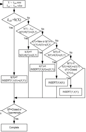
The optimal path for global path planning can be obtained using D* algorithm flow chart as shown in Fig.1.
Fig. 1 Complete flowchart of D* algorithm
C. Local Path Planning
Fig. 2 shows the condition when D* re-planning the path. When an obstacle is detected, A*and D* algorithms restart the general search process. This is equivalent to find a “broken” arc r in an initial path e of a graph. e is a time or length optimal path between an starting node and a goal node . Arc r is defined by two nodes: (current node), which represents the current robot position and y (next node), which represents the next robot’s movement destination. Nodes { , , and y }∈N. Every node connected to the current node , except y, is used to generate a new partial solution path set. Each new path ycƼ from the new path set is added to the D* OPEN list. The
OPEN list contains a set of partial solution paths that are expanded until is reached. Thus, a first path/node expansion implies to generate new partial solution paths ycƼ composed of nodes included in e∗=( , , )⊂ e and the set of neighbour nodes connected to . Arc r is ignored and cannot be a part of any solution.
Fig. 2 D* re-planning path
Plan A shows an initial path e. is the current node and r the “broken” arc. Plan B shows the algorithm to find the path until it reaches the goal. Plan C shows final re-planed path using D* algorithm.
The whole search process ends when:
1) y or another node included in the original path e is found and the rest of partial paths (solutions) included in the OPEN list have a higher f value. f = g + h, where g is the accumulated path cost and h is the heuristic value that estimates path cost from to (see Fig. 2). Usually, function f implements the Euclidean distance.
2) The goal node is reached and the rest of partial paths have a higher f value. This is equivalent to a brute-force method and represents the worst case.
3) The OPEN list is empty. This means that there are no solutions without r .
Fig. 3 Example of local path planning
Fig. 3 shows path-planning example for loc avoidance applied on a subsection of the search spa
III. SYSTEM CONFIGURATION
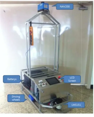
Fig. 4 shows the system configuration for exp this paper. Tank-800 industrial computer is use controller. Half PCI MMC Board connects the computer with motor driver, all inputs an 200W/3000 rpm BLDC motor are used to move wheel. For monitoring, LCD screen is used. A systems are powered by 2x 12V/8Ah batteries.
Fig. 4 AGV system
For positioning the AGV in absolute coordinat is used. NAV200 system is a laser-based position that returns an absolute position of the scanner wit a user-defined local coordinate frame. Nav2 comprises of two main units, a laser scanner Transputer Position Unit (TPU). This lase continuously rotates 360 degrees to scan the ref then sends the information to the TPU to co scanner’s position. This system can provide accur mm with an update rate up to 8Hz [16]. Th navigation system is shown in Fig. 5.
local obstacle space.
experiment in sed for main the industrial and outputs. ve the driving All of those
ate, NAV200 ioning system ith respect to v200 system r unit and a aser scanner reflectors and compute the uracy up to 1 The NAV200
Fig.5 NAV200 laser navigation s
For obstacle detection, the laser m LMS151 is employed. LMS151 system is system that recognizes obstacles in 270 LMS151 is an electro-sensitive distance for stand-alone or network operation. applications in which precise, electro-sen of contours and surroundings are require to realize systems, for instance, for col building surveillance or for access monito up to 50 m and rotation frequency is 2 measurement system is shown in Fig. 6.
Fig. 6 LMS151 laser measuremen
IV. SIMULATION AND EXPERIMEN
A. Simulation Results
Simulation is done to confirm the f Algorithm as shown in Fig.7.
START
GOAL
Fig.7 Simulation result for path
The map is obtained by converting t into simple grid map. In this simul represented as one unit square. To simpli
36
n scanner
measurement system is a laser measurement 270 degrees scan. The ce measurement system on. It is suitable for sensitive measurements ired. It is also possible ollision protection, for itoring. Scanning range s 25 Hz. The LMS151
ent scanner
ENTAL RESULTS
feasibility of the D*
ath planning
37 this simulation, one grid size 30 cm x 30 cm is chosen. The
optimal path that is calculated by D* algorithm is shown in Fig.7.The slashed area represents the known obstacle in environment. The darker area represents the higher cost, and the lighter area represents the lower cost. The dot line represents the shortest trajectory from start position to the goal position.
B. Experimental Results
Fig. 8 shows the comparison between simulation result and real experiment result. Fig. 8 shows that the simulation result is similar with experimental result. They show that the proposed algorithm successfully generates the optimal path and the AGV can reach the goal position without colliding with the obstacles. Numbers on x axis and y axis in Fig.8 is in grid number
Fig. 8 Simulation and experimental results using the proposed algorithm
Fig. 9 shows the error between simulation and real experimental result.
-5 -4 -3 -2 -1 0 1 2 3 4 5 6 7 8 9 10
0 50 100 150 200
E
rr
o
r
(c
m
)
Fig. 9 Error between simulation and experimental results
The error between simulation and experimental results is defined as:
Â
= [(
c−
) + (
c−
) ]
Where, e is position error, , are AGVposition from simulation result and c , c are AGV position from experimental result. The error is bounded within ±5cm. Therefore, it shows that the proposed algorithm can be successfully implemented in real system.
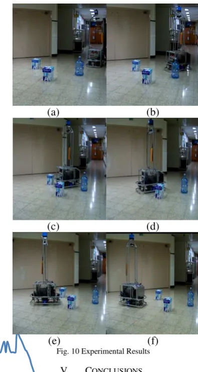
Fig. 10 shows the experimental results using D* algorithm. Fig. 10(a) shows the experimental AGV using the laser
scanner LMS-151 and laser navigation sensor NAV-200 in start position. The AGV calculates the optimal path to the goal position using D* algorithm. After generating the optimal path, the AGV moves forward while it is scanning the environment to update the information according to changing of environment and obstacle as shown in Fig. 10(b). When AGV finds some new obstacles that are different from the given map information such as unknown obstacle as shown in Fig. 10(c), it adds the information to its map and re-plans a new shortest path from its current coordinates to the given goal coordinates as shown in Figs. 10(d) ~ (e). It repeats the process until it reaches the goal position as shown in Fig. 10(f).
(a)
(b)
(c)
(d)
(e)
(f)
Fig. 10 Experimental Results
V. CONCLUSIONS
38
ACKNOWLEDGMENT
This research was supported by a grant from Construction Technology Innovation Program (CTIP) funded by Ministry of Land, Transportation and Maritime Affairs (MLTM) of Korean government.
REFERENCES
[1] T. Loazno-Perez and M.A. Weslsy, “An Algorithm for Planning
Collision-free Paths among Polyhedrial Obstacles,” Commun. ACM, pp. 560-570,1979.
[2] O. Khatib, “Real-Time Obstacle Avoidance for manipulator and
Mobile Robots,” The International Journal of Robotic Research, MIT Press, Cambridge, pp. 90-98,1986.
[3] E. Rimon and E.E. Koditschek, “Exact Robot Navigation Using
Artificial Potential Functions,” IEEE Transactions on Robotics and Automation, Vol. 8, No. 5, pp. 501-518,October, 1992.
[4] H.I. Yoo and B.S. Kang, “Precise Motion Control of a Mobile Robot
Based on Potential Field Method,” The KSME 2008 Dynamics and Control spring annual meeting, pp. 177-180, 2008.
[5] M.G. Park and M.C. Lee, “A New Technique to Escape Local
Minimum in Artificial Potential Field Based Path Planning,” KSME International Journal, Vol.17, No.12,pp. 1876-1885, 2003.
[6] J. Bruce and M. Veloso, “Real-Time Randomized Path Planning for
Robot Navigation,” Proc. of the 2002 IEEE/RSJ Int. Conference on Intelligent Robots and Systems EPFL, Lausanne, Switzerland,pp. 2383-2388,October, 2002.
[7] K. Konolige, “A Gradient Method for Realtime Robot Control,” Proc.
of International Conf. on Intelligent Robots and Systems, pp. 639-646, 2000.
[8] J. Borenstein and Y. Koren, “The Vector Field Histogram-Fast
Obstacle Avoidance for mobile Robots,” IEEE Journal of Robotics and Automation Vol. 7, No. 3, pp. 278-288, June 1991.
[9] D. Fox, W. Burgard and S. Thrun, “The Dynamic Window Approach
to Collision Avoidance,” IEEE Robotics and Automation, Vol. 4, No. 1,pp. 23-33, 1997.
[10] R. Simmons, “The Curvature-Velocity Method for Local Obstacle
Avoidance,” Proc. Of International Conf. on Robotics and Automation, pp. 3375-3382,1996.
[11] H.J. Kim, D.H. Shim and S. Sastry, “Nonlinear Model Predictive
Tracking Control for Rotorcraft-Based Unmanned Aerial Vehicles,” Proceedings of the American Control Conference, Anchorage, AK pp. 8-10,May, 2002.
[12] P. Ogren and N.E. Leonard, “A Convergent Dynamic Window
Approach to Obstacle Avoidance,” IEEE Transactions on Robotics and Automation, pp. 188-195, 2003.
[13] C. Stachniss and W. Burgard, “An Integrated Approach to
Goal-Directed Obstacle Avoidance Under Dynamic Constraints for Dynamic Environments,” Proceedings of the 2002 IEEE/RSJ, intl, Conference on Intelligent Robots and Systems EPFL, Lausanne, Switzerland, pp. 508-513, October, 2002.
[14] A. Stentz, “Optimal and Efficient Path Planning for Partially-known
Environments”, in: Proceedings of the IEEE International Conference on Robotics and Automation (ICRA’94), Vol. 4, pp. 3310-3317, 1994.
[15] N.J. Nilsson, “Principles of Artificial Intelligence”, Tioga Publishing
Company, pp. 76-79, 1980.
[16] “NAV200 Positioning System for Navigation Support Technical
Description,” SICK.
[17] T.L. Bui et al, “AGV Trajectory Control Based on Laser Sensor
Navigation”, International Journal of Science and Engineering, Vol. 4(1), pp. 39-43, 2013.
[18] P.S. Pratama, Sang K..J., Soon S.P, S.B. Kim, “Moving Object