O R I G I N A L A R T I C L E
Strength and deformability of corroded steel plates
under quasi-static tensile load
Md. Mobesher AhmmadÆY. Sumi
Received: 25 April 2009 / Accepted: 2 August 2009 / Published online: 10 September 2009 JASNAOE 2009
Abstract The objective of this study was to estimate the strength and deformability of corroded steel plates under quasi-static uniaxial tension. In order to accurately simulate this problem, we first estimated the true stress–strain rela-tionship of a flat steel plate by introducing a vision sensor system to the deformation measurements in tensile tests. The measured true stress–stain relationship was then applied to a series of nonlinear implicit three-dimensional finite element analyses using commercial code LS-DYNA. The strength and deformability of steel plates with various pit sizes, degrees of pitting intensity, and general corrosion were estimated both experimentally and numerically. The failure strain in relation to the finite element mesh size used in the analyses was clarified. Two different steels having yield ratios of 0.657 and 0.841 were prepared to examine the material effects on corrosion damage. The strength and deformability did not show a clear dependence on the yield ratios of the present two materials, whereas a clear depen-dence was shown with respect to the surface configuration such as the minimum cross-sectional area of the specimens, the maximum depth of the pit cusp from the mean corrosion diminution level, and pitting patterns. Empirical formulae for the reduction of deformability and the reduction of energy absorption of pitted plates were proposed which may be useful in strength assessment when examining the structural integrity of aged corroded structures.
Keywords StrengthDeformabilityQuasi-static load Pitting corrosionGeneral corrosionTrue stress–strain relationshipMesh sensitivityYield ratio
1 Introduction
Marine structures are subjected to age-related deterioration such as corrosion wastage, fatigue cracking, or mechanical damage during their service life. These forms of damage can give rise to significant issues in terms of safety, health, environment, and financial costs. It is thus of great importance to develop advanced technologies that can assist proper management and control of such age-related deterioration [1]. In order to assess the structural perfor-mance of aged ships, it is of essential importance to predict the strength and absorbing energy during the collapse and/ or fracture of corroded plates.
Nowadays, numerical simulation is being used to replacing time-consuming and expensive experimental work. An exact simulation of tension tests requires a complete true stress–strain relationship. Here we first estimate the true stress–strain relationship of steel plate with a rectangular cross section. A vision sensor system is employed to estimate the deformation field from the specimen surface from which an averaged least cross-sec-tional area and a correction factor due to the triaxial stress state can be evaluated. The measured true stress–strain relationship is then applied to an elastoplastic material model of LS-DYNA (Livermore Software Technology, Livermore, CA, USA) to assess the strength and defor-mability of corroded steel plates.
A great number of research projects have been carried out on the structural integrity of aged ships. Nakai et al. [2] studied the strength reduction due to periodical array of Md. M. Ahmmad
Graduate School of Engineering,
Yokohama National University, 79-5 Tokiwadai, Hodogaya-ku, Yokohama 240-8501, Japan
Y. Sumi (&)
Faculty of Engineering, Systems Design for Ocean-Space, Yokohama National University, 79-5 Tokiwadai, Hodogaya-ku, Yokohama 240-8501, Japan e-mail: [email protected]
pits, while Sumi [3] investigated the self-similarity of surface corrosion experimentally. Paik et al.[4,5] studied the ultimate strength of pitted plates under axial com-pression and in-plane shear. They also derived empirical formulae for predicting the ultimate compressive strength and shear strength of pitted plates. Yamamoto [6] discussed the simulation procedure for pitting corrosion by using probabilistic models.
In the present article, we shall discuss the geometrical effect on the strength and deformability of steel plates with various pit sizes, degrees of pitting intensity, and with general corrosion. Using the probabilistic models proposed by Yamamoto and Ikegami [7], pitted surfaces of various pitting intensities were simulated and tested to obtain strength and deformability both experimentally, and numerically. The shape of pits is assumed to be conical. Empirical formulae are proposed to estimate the reductions in deformability and energy absorption capacity, and these were verified by experimental and numerical results. In the case of general corrosion, replica specimens were made to simulate corroded surfaces sampled from an aged heavy oil carrier. In experiments, the geometries of corroded surfaces were generated by a computer-aided design (CAD) system and were mechanically processed by a numerically con-trolled (NC) milling machine in a computer-aided manu-facturing (CAM) system. Investigations were made for two different steels with the same ultimate strength, but having yield ratios of 0.657 (steel A) and 0.841 (steel B), to identify the material effects of corrosion damage. Note that the former type of steel is commonly used for marine structures.
2 Measurement of true stress–strain relationship
The true stress–strain relationship, including the material response in both pre- and postplastic localization phases, is necessary as input for numerical analyses. In some cases, structural analysts use a power law stress–strain relation-ship. It has been demonstrated that power law stress–strain curves for certain steels may overestimate the actual stress– strain curve at low plastic strain, while underestimating it in the later stages [8]. For thick sections, the true stress–strain relationship can conveniently be determined by using a round tensile bar, while for thin sections it is better to use specimens with a rectangular cross section [9]. However, strain measurement becomes complicated, especially for flat tensile specimens, due to the inhomogeneous strain field and triaxial stress state. Two practical difficulties can be mentioned here. The first problem is the measurement of the instantaneous area of minimum cross section after necking. During plastic instability, the cross section at the largest deformed zone forms a cushion-like shape [10], so that it is
difficult to measure the cross-sectional area at the neck. The second challenge is the measurement ofa/R, whereais the half-thickness andRis the radius of curvature of the surface at the neck (see Fig.1), to estimate a correction factor, e.g., Bridgman [11] and Ostsemin [12] correction factors for the triaxial stress condition after necking.
2.1 True stress and true strain
For any stage of deformation, true stress and true strain are defined by: whereA,F,l0, andlare the instantaneous area, the applied force, the initial length of a very small gauge length (say 1 mm) at the possible necking zone, and its deformed length, respectively. As long as uniform deformation occurs, the true stress and strain can be calculated in terms of engineering stress,re, and engineering strain, ee, by:
eT¼ln 1ð þeeÞ; rT¼reð1þeeÞ ð2Þ
The effective strain,e; after bifurcation was calculated by Scheider et al.[10] as: whereeIandeIIare the true strains in the specimen’s length and width directions, respectively. Usually bifurcation phenomena occur soon after the maximum load. In our calculations, we shall use Eq.3to measure the true strain. After the initiation of necking, true stress can be cal-culated by:
whereeIIIis the strain in the thickness direction. In the case of uniform deformation, Eq. 4can be calculated as: Fig. 1 Illustration of necked geometry.ahalf-thickness of the neck,
rT¼
F A0
expðeIÞ ð5Þ
In practice, the axial strain over the cross section, as shown in Fig.2a, is not uniform, so that an average true stress can be obtained from Eq.6 by measuring an average axial strain,eI (see Fig.2b):
rT¼
F A0
expðeIÞ ð6Þ
The true equivalent stress after the correction due to the triaxial stress state can be expressed as:
req¼ whereCBandCOare two analytical correction factors that can be used for rectangular cross-section specimens after the initiation of necking. These factors are given by Bridgman [11]: whereaandRare defined as illustrated in Fig.1, in which the solid bold line represents the upper surface of the centerline section of the neck. The correction factors CB andCOdepend on a parameter,a/R, given by: thickness,a0, is estimated at a distancebfrom the center of the neck (see Fig.1). The continuous values of the thickness can be estimated by the surface strains in the
length and width directions by the vision sensor by applying the following relations:
a¼a0expðeIIIÞ ¼a0expðeIeIIÞ ð11Þ
a0¼a0expðe0IIIÞ ¼a0expðe0Ie0IIÞ: ð12Þ
2.2 Experimental procedures
The geometry of the flat specimen is shown in Fig.3a. The specimen surface is prepared as shown in Fig. 3b: white dots on permanent black ink are painted on the specimen. The relatively long length, 40 mm, of the measuring zone is designed so that necking occurs within this range without introducing any imperfections to the test specimen.
Figure4 shows the experimental setup. The mono-chromic vision sensor traces the white dots during the experiment. Since the white paint should have high deformability to follow the large deformation, we use correction fluid for the white dots. An extensometer is also used to measure the strain of gauge length 100 mm. Having read the position of the dots on the specimen surface, these digital data are converted to analog data by a D/A con-verter, where the deformation data and load data are syn-chronized on a personal computer through a voltage signal interface. A programmable logical controller is used to synchronize the whole system.
2.3 Test results
In this study we observe that uniform deformation occurs until the first bifurcation (initiation of diffuse neck) at strain 0.25, and the strain at maximum load is 0.16 for steel A. The correction factor due to the triaxial stress state becomes effective after the second bifurcation at strain
Fig. 2 aDeformed grid on the surface of necked zone.bEstimation of average axial strainðeIÞ:CLcenter line
Fig. 3 aThe tensile specimen (all dimensions in mm).bWhite dots
0.45. The correction factor varies from 1 to 1.03, which implies that the true stress is reduced by 0–3% after the second bifurcation. Applying the procedure discussed in the previous subsection, the true stress–strain relationships are obtained for steel A and steel B as illustrated in Fig.5a and b. Note that the true stress–strain relationships with the Ostsemin correction factor are used for the finite element analyses in the subsequent sections.
3 Numerical analysis
Numerical analyses were carried out by using a nonlinear implicit finite element code, LS-DYNA, as the problem is a quasi-static type. The constitutive material model is an elastoplastic material where an arbitrary stress versus strain curve can be defined. This material model is based on the J2flow theory with isotropic hardening [14].
3.1 Finite element model and material properties
The basic problem that was analyzed is the quasi-static uniaxial extension of a rectangular bar, as shown in Fig.6. Due to the symmetry, only one octant of the specimen is analyzed using the finite model discretized by 8-node brick elements as shown in Fig.6b. A constant velocity,V(t), of
3 mm/min is prescribed in the x direction. The material properties are listed in Table1, and the strain hardening is defined by the true stress–strain curves illustrated in Fig.5a and b. The fracture strain,ef, is measured by:
ef ¼ln
A0
Af
ð13Þ where Af is the projected fracture surface area measured after the experiments.
3.2 The effect of mesh size
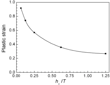
Mesh size effects are crucial in the failure analyses of structures. In general, a finer mesh size is needed for accurate results when large deformation accompanies strain localization. However, a significant complication arises because of mesh size sensitivity whereby the strain to failure increases on refining the mesh. The failure strain of the finite element analyses is defined as the maximum plastic strain, i.e., when the nominal strain reaches 0.284 (steel A), at which the flat specimen failed in the experiments. In Fig.7, we compare the failure strains of five finite element models at the same nominal strain at failure. In these cases, we only change the ele-ment size, hx, in the loading direction, keeping the mesh
size constant at 1 mm in the remaining two directions, hy
andhz, because their effect is not so significant. From the
figure, it can be seen that the finer the mesh size the higher the maximum plastic strain. Figure8 represents a comparison of experimental and numerical nominal stress–strain relationships for a flat plate of steel A. The element size is 0.59192 (mm). Similar results were
obtained for steel B, for which the numerical results agree well with the experimental values.
4 Pitting corrosion and its effect
Pitting is an extremely localized form of corrosion. It typ-ically occurs in the bottom plating of oil tankers, in struc-tural details that trap water, and in the hold frames of cargo Fig. 4 Experimental setup and vision system.D/Adigital to analog
holds of bulk carriers that carry coal and iron ore. When the effect of corrosion on local strength and deformability is considered, pitting corrosion is of great concern. The effect of pitting corrosion on the compressive and shear strengths has been studied both experimentally and numerically by several researchers. In the present study, we shall investi-gate in detail the tensile strength, focusing attention on the deformability and energy absorption capacity.
4.1 Simulation of plates with a single pit and periodical arrays of pits
In this subsection, we shall discuss the simulation procedure of steel plates with a single pit or a periodical array of pits. In addition, we shall observe the effect of pit size on the nominal stress–strain relationship of plates with a single pit. To estimate the effect of pit size on strength and deforma-bility, we consider three different pit sizes (diameters of 10, 20, and 40 mm) whose depth-to-diameter ratio is 1:8.
At first, the true stress–strain relationships of steels A and B will be applied to specimens with surface pit con-figurations as specified in Table2. Figure9a and b show the specimens and mesh pattern of the one quadrant of the model, respectively. The mesh sensitivity within the pit cusp was analyzed by changing the mesh size along the thickness direction, while those in the other directions remained constant; the radial mesh size and the circum-ferential mesh angle were 0.5 mm and 4.5, respectively.
By refining the mesh size within the pit cusp, the maximum plastic strain in the longitudinal direction calculated at nominal failure strain, 0.175, sharply increased, as shown in Fig.10. The experimental and numerical results of the nominal stress–strain relationship of steel A are shown in Fig.11a and b, respectively, in which we can observe good agreement. Similar results were also obtained for steel B.
Nakai et al. [2] and Sumi [3] have experimentally investigated the strength and deformability of steel plates with periodical arrays of surface pits (see Fig.12a–d). Periodical pits were made on both surfaces of a plate and they were arranged asymmetrically with respect to the middle plane of the specimen (see Fig.12e). To make a finite element model, we first generated an array of points that describes the surfaces with these pits. From this point data we can obtain a nonuniform rational B-spline (NURBS) surface [15] that can be discretized using iso-mesh. Having obtained the data for the front and back surfaces, solid elements (8-node hexahedrons) can be generated by a sweeping action, as shown in Fig.12f. The
Fig. 6 Finite element model of a flat specimen. a the one-eighth analyzed,bmesh and element pattern
Table 1 Material properties
Material Yield strength (N/mm2)
Tensile strength (N/mm2)
Y/T ratio E (GPa) Poisson’s ratio
Elongation (%)
Failure strain
Steel A 344 523 0.657 206.5 0.3 28.41 0.92
Steel B 440 523 0.841 204.5 0.3 28.94 0.90
SM490A 325 513 0.634 206 0.3 32.46
Y/Tyield strength to tensile strength ratio,EYoung’s modulus
Fig. 7 Effect of mesh size on maximum plastic strain at failure (steel A).hxlength of each element,Tsample thickness
numerical and experimental nominal stress–strain curves of steels A and B are shown in Fig.13. Here the failure strain is defined as 0.7, as the element size is 1 91 94 mm. A
good agreement is observed among experimental and numerical nominal stress–strain curves until the strain reaches about 0.15 (see Fig. 13).
4.2 Validation of numerical results
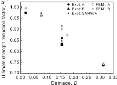
Nakai et al. [2] and Paik et al. [4] have confirmed that the ultimate strength of a steel plate with pitting corrosion is governed by the smallest cross-sectional area. Here we also consider the ultimate strength reduction factor, Ru, as a function of damage. The damage value depends on the smallest cross-sectional area, Ap, due to surface pits and can be defined as:
Damage; Dm¼
A0Ap
A0 ð
14Þ whereA0is the intact sectional area, andRuis defined as: Ru ¼
rup
ru0 ð
15Þ whereru0andrupare the ultimate tensile strength of intact plates and pitted plates, respectively. Figure14shows that the strength reduction factor decreases with increasing damage of steels A and B. Sumi [3] experimentally investigated the strength and deformability of artificially pitted plates of SM490A steel with a yield ratio 0.63, whose results as well as the present numerical results are presented in this section (see Figs.14, 15,16). Note that the damage value of all models with periodical array of surfaces pits is 0.15625. In Fig.14,Ru, slightly decreases with the increase of pit number for periodical pits.
We define the reduction of deformability, Rd, due to surface pits as:
Rd ¼
ep
e0 ð
16Þ wheree0andepare the total elongation of flat and pitted specimens, respectively, under uniaxial tension. Figure15
shows the reduction of deformability, Rd, as a function of damage of plates with a single pit and a periodical array of pits obtained by experiments and simulations. It is observed in single-pit problems that the deformability decreases with increasing damage, while in periodical-pit problems it increases with the total number of pits.
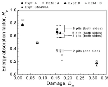
Let us introduce another parameter—the reduction of energy absorption,Re, as:
Re¼
Ep
E0 ð
17Þ whereE0andEpare the total energy absorbed by an intact flat plate and a pitted plate, respectively, in uniaxial Table 2 List of tensile test specimens of flat plate and plate with a
single pit or a periodical array of pits
No. Material No. of pits Pit diameter (mm)
Side 1 Side 2
A3-F3 A 0 0 0
A3-F6 A 0 0 0
A3-F8 A 0 0 0
A3-10 A 1 0 10
A3-20 A 1 0 20
A3-40 A 1 0 40
A3-20-8 (1) A 8 8 20
A3-20-8 (2) A 8 8 20
B3-F1 B 0 0 0
B3-10 B 1 0 10
B3-20 B 1 0 20
B3-40 B 1 0 40
B3-20-8 (1) B 8 8 20
B3-20-8 (2) B 8 8 20
SM490A-20-2a SM490A 2 0 20 SM490A-20-4a SM490A 4 4 20 SM490A-20-4a SM490A 6 6 20 SM490A-20-8a SM490A 8 8 20
All specimen dimensions are as shown in Fig.3a The diameter to depth ratio of all pits is 8:1 a
From Sumi [3]
Fig. 9 Pitting surfaces:aspecimens with a single pit,bmesh pattern of the quadrant of the processed zone (5092098 mm)
tension. The energy can be measured by integrating the area under the nominal stress–strain curves. Figure16
shows the reduction of energy absorption,Re, as a function of damage, Dm, for various pitted plates. Here, also, Re decreases with the increase in damage value in single-pit problems, and it increases with the increase in the number of pits in periodical-pit problems.
From Figs.14, 15, 16, it can easily be seen that the deformability and energy absorption capacity reduce con-siderably with increasing pit size, while the strength
reduces moderately. Also, we can observe that the differ-ences in the reduction of the strength, deformability, and energy absorbing capacity of steels A and B are insignifi-cant. In general, we observed a good agreement between the numerical and experimental results for the pit problems.
Fig. 11 Nominal stress–strain curves for various single-pit specimens made of steel A.aExperimental values,bcalculated values
Fig. 12 Periodical array of pits;apits on one side,b–dpits arranged asymmetrically on both sides,etest specimen with periodical pits and pit geometry, andfmesh pattern of pitted model
Fig. 13 Verification of numerical stress–strain relationships using experimental data for plates with periodical array of surface pits
5 Simulation of plates with random arrays of pits
Yamamoto and Ikegami [7] discussed the mathematical models by which the surface condition of structural members with corrosion pits can be generated. According to their probabilistic models, the generation and progress of corrosion involves the following three sequential pro-cesses: the generation of active pitting points, the genera-tion of progressive pitting points, and the progress of pitting points. The life of a paint coating can be assumed to follow a lognormal distribution given by:
fT0ðtÞ ¼ ffiffiffiffiffiffi1 the mean and standard deviation of ln(T0). Active pitting points are generated after time,T0. The transition time,Tr,
from active pitting points to progressive pitting points is assumed to follow an exponential distribution:
gTrðtÞ ¼aexpðatÞ ð19Þ where a is the inverse of the mean transition time. The progress behavior of pitting points after generation is expressed as:
zðsÞ ¼csb ð20Þ
where s is the time elapsed after the generation of progressive pitting points with the coefficients c and b. Coefficientcis determined as a lognormal distribution: hcðcÞ ¼ ffiffiffiffiffiffi1
where lc andrc are the mean and standard deviation of
ln(c). The value of coefficientbis considered to vary from 1 to 1/3, depending on the materials and the corrosive environment.
In this study, the shape of the corrosion pit is defined by the following shape function:
The position vectors of the pit center and that of an arbitrary surface point are denoted by x0 and x, respectively. The depth and diameter of a corrosion pit at x0are represented byz0andD0. The ratio of the diameter to the depth of the pits was observed to vary from 6 to 10. It is assumed thatv0is a random variable that follows a normal distribution given by:
We shall consider a plate taken from a hold frame of a bulk carrier with dimensions of 200980916 mm. Having generated various stochastic pitting patterns due to corrosion, we shall simulate the resulting strength and deformability. The numerically generated corroded surface depends considerably on the number of possible pitting points on the surface. We assume that the maximum den-sity of pitting initiation points is, approximately, 1 pit/ 53 mm2. The assumed parameters of the probabilistic models are given in Table3.
Fig. 15 The reduction of deformability,Rd, as a function of damage for plates with a single pit and periodical pits under uniaxial tension. The samples had one pit unless otherwise stated
5.1 Statistics of the corrosion condition
Once we obtain the probabilistic parameters, we can sim-ulate the corroded surface by using the shape function given by Eq.22. Let us discuss some statistical charac-teristics of pitting corrosion. Average corrosion diminution is defined as the average thickness loss due to corrosion in each year. If z(x) denotes the depth of corrosion at any point x(x, y) on the surface, we can obtain the average corrosion diminution,zavg, by:
zavg¼E½zðx;yÞ ¼
whereM andNare the number of sections in thexandy directions. In general, Eq.24 can be evaluated from dis-crete point data. Figure17shows the thickness diminution of five sampled plates over 20 years obtained from the same probabilistic parameters as those listed in Table3. Thickness diminution progresses linearly after the failure of the coating protection system (CPS). In this case, thickness diminution starts after approximately 5 years.
The degree of pitting intensity (DOP) is defined as the ratio of the pitted surface area to the whole surface area. According to the unified rules of the International Asso-ciation of Classification Societies (IACS), if the DOP in an area where coating is required is higher than 15%, then thickness measurement is required to check the extent of corrosion. Figure17 shows the increase in the degree of pitting intensity with a structure’s increasing age. During the first 2.5–10 years, DOP increases rapidly because of the quick deterioration of the protective coating system.
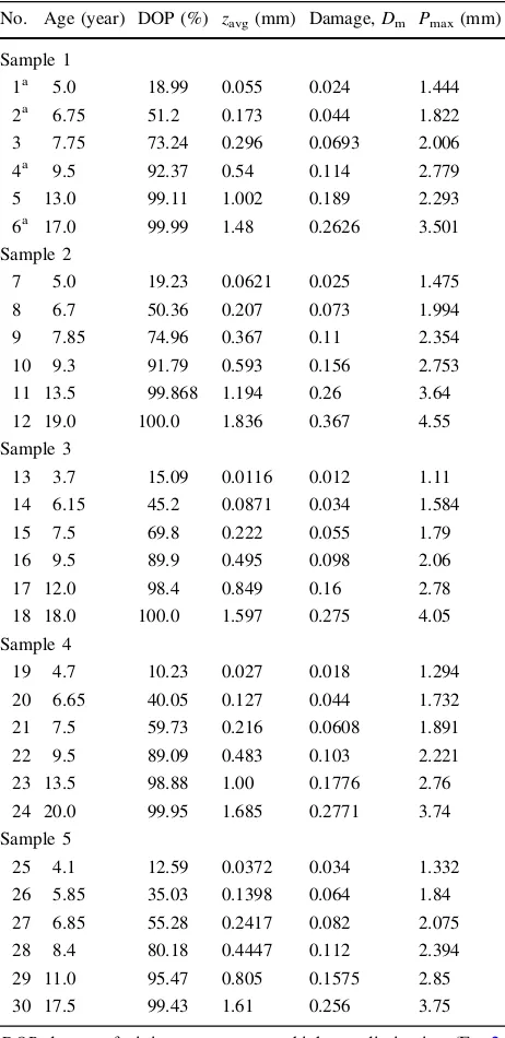
We shall investigate the strength and deformability of these five sampled plates at various corrosion stages. For finite element simulations, we intend to select six charac-teristic points from each sample. The various characteris-tics of numerical calculations and experiments are shown in Table4. We carried out four experiments for the pos-sible validation of the corresponding finite element results. 5.2 Simulated corrosion surfaces based
on a probabilistic model
In order to simulate the strength and deformability of corroded plate, a question may arise as to how the results
may change with the plate width. This problem has been discussed by Nakai et al. [2] by using small and wide specimens, where the width and gauge length were 80 and 200 mm for small specimens and 240 and 400 mm for wide specimens. Although there is some scatter in their experimental data, the strength reduction can basically be estimated in both cases by using the area of minimum cross section,Ap, perpendicular to the loading axis. On the other hand, deformability obviously depends on the definition of the gauge length of the plate. They also observed the same level of deformability in a small specimen as that in a wide plate when the elongation of a wide plate was measured in a similar gauge length along the fracture zone. From these observations, we decided to simulate the mechanical behavior of an area of 200980 mm in the following analyses.
The surface corrosion conditions of the corroded area are simulated for six different DOPs from each sample. Figure18a–f show the simulated corrosion conditions of sample 1. Figure19shows the test specimens with 19, 51, 92, and 100% DOP (sample 1). Note that the sizes of the processed area of the test specimens are self-similar with a scale factor of 0.5 with respect to the original size. According to Sumi [3], a self-similar specimen behaves similarly within this scaling factor if the same quantity of geometrical information is contained in both models.
The procedure of surface processing of test specimens is briefly explained. We first make an array of points that describe the corroded surface based on probabilistic cor-rosion models. From this data we obtained a NURBS surface generated by CAD software Rhinoceros (McNeel, Seattle, WA, USA). The generated surface was imported into CAM software Mastercam (CNC, Tolland, CT, USA) to process the specimen surfaces for the experiments, and it was also imported into Patran (MSC, Santa Ana, CA, USA) for the finite element analyses. The top and the bottom Table 3 Parameters of probabilistic models [7]
l0 r0 1/a 1/b lc rc
Bulkhead (cargo hold) 1.701 0.68 1.90 2.0 0.0374 0.3853
l0, r0, mean and standard deviation of ln(T0); a, b, parameters defined by Eqs.19and 20;lc,rc, mean and standard deviation of
ln(c) in Eq.21
surfaces as well as the internal surface of the specimen are generated so that they are discretized by isomesh. The three-dimensional solid finite element model was obtained by the same procedure discussed in Sect.4.1. It consists of 16720 8-node solid elements with a minimum size in the processed area of 0.591 91 mm. We control the
mini-mum element size in the thickness direction by defining a two-layered model with an internal surface 1 mm below the cusp of the deepest pit.
The accuracy of the geometries of the test specimens and finite element models were confirmed by comparing them with the original data of the probabilistic corrosion model. Figure 20compares the various thickness distribu-tions of the finite element models and the test specimens along their length. These are obtained by:
E½zWðxÞ ¼ 1 W
Z
W=2
W=2
zðx;yÞdy ð25Þ
whereW is the width of the corroded plate, andz(x,y) is the corrosion diminution at point (x,y) on the surface. The finite element data coincides with the original data. Having Table 4 Characteristics of the simulated plates and test specimens
with random pits
No. Age (year) DOP (%) zavg(mm) Damage,Dm Pmax(mm)
Sample 1
1a 5.0 18.99 0.055 0.024 1.444 2a 6.75 51.2 0.173 0.044 1.822 3 7.75 73.24 0.296 0.0693 2.006 4a 9.5 92.37 0.54 0.114 2.779 5 13.0 99.11 1.002 0.189 2.293 6a 17.0 99.99 1.48 0.2626 3.501 Sample 2
7 5.0 19.23 0.0621 0.025 1.475 8 6.7 50.36 0.207 0.073 1.994 9 7.85 74.96 0.367 0.11 2.354 10 9.3 91.79 0.593 0.156 2.753 11 13.5 99.868 1.194 0.26 3.64 12 19.0 100.0 1.836 0.367 4.55 Sample 3
13 3.7 15.09 0.0116 0.012 1.11 14 6.15 45.2 0.0871 0.034 1.584 15 7.5 69.8 0.222 0.055 1.79 16 9.5 89.9 0.495 0.098 2.06 17 12.0 98.4 0.849 0.16 2.78 18 18.0 100.0 1.597 0.275 4.05 Sample 4
19 4.7 10.23 0.027 0.018 1.294 20 6.65 40.05 0.127 0.044 1.732 21 7.5 59.73 0.216 0.0608 1.891 22 9.5 89.09 0.483 0.103 2.221 23 13.5 98.88 1.00 0.1776 2.76 24 20.0 99.95 1.685 0.2771 3.74 Sample 5
25 4.1 12.59 0.0372 0.034 1.332 26 5.85 35.03 0.1398 0.064 1.84 27 6.85 55.28 0.2417 0.082 2.075 28 8.4 80.18 0.4447 0.112 2.394 29 11.0 95.47 0.805 0.1575 2.85 30 17.5 99.43 1.61 0.256 3.75
DOPdegree of pitting,zavgaverage thickness diminution (Eq.24), Dmdamage,Pmaxmaximum depth of pit
a
Test with steel A
Fig. 18 Simulated pitting corrosion surfaces (sample 1)
used a cutting tool of 2-mm diameter for processing the test specimens, a slight difference is observed with the original data as shown in the figure.
5.3 Results and discussions
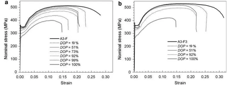
Figure21a, b show the nominal stress–strain curves of steel A obtained by simulations and experiments (sample 1). Generally speaking, strength and deformability decrease with increasing DOP. If we compare the numerical and experimental results, we can see that the experimental results give approximately 3% higher strength values than those generated by the numerical calculations. Of course, we observe a slight variation of strength and deformability in different tests of the same material (Y/T=0.657). Note
that all finite element analyses with steel A were carried out for a constant ultimate strength of 513 MPa.
Figure22a–d show comparisons of the location of fail-ure in simulations and experiments for four different cor-rosion conditions (sample 1). In the numerical simulations, considering the mesh size sensitivity shown in Fig.7, element failure is assumed when the strain of an element reaches 0.92, and the corresponding element stiffness is set to zero afterwards. The location of maximum pit depth, the
minimum cross-sectional area, and the location of failure in numerical and experimental specimens are listed in Table5
for sample 1. For numerical models with their DOPs of 19, 92, 99, and 100%, failure occurs at or near the minimum cross-sectional area, while for DOP 51 and 73% it occurs along the favorable shear band formed prior to the failure. We can see that the simulated failure locations certainly coincide with their experimental counterparts.
To understand the cause of failure, we have monitored the whole process of plastic deformation in simulations as well as in experiments. We observe that stress concentra-tion occurs at each pit cusp during the entire loading pro-cess. After the maximum load, unloading starts from both ends of the specimen. A shear band forms at a favorable direction in relation to the pit orientation, which leads to failure initiation from the minimum thickness on the shear band.
In Sect. 4.2we discussed the strength reduction factor for plates with a single pit and a periodical array of pits as a function of damage, which is estimated based on the smallest cross-sectional area. In the case of the probabi-listic corrosion model, the total number of pits as well as the damage increases with time. Figure23 shows the experimental and numerical results of ultimate strength reduction with increasing damage due to pitting corrosion for all pitted models of steels A and SM490A. The strength reduces approximately 20% within 20 years. It was con-firmed that the tensile strength of pitted plates can be predicted by the empirical formula proposed by Paik et al. [4] for the compressive strength of pitted plates:
Ru ¼ ð1DmÞ0:73 ð26Þ
How much does deformability reduce with the progress of corrosion? Which parameters does it depend on? We have investigated the answers of these questions. We found that deformability does not have a good correlation with the maximum pit depth (Pmax) or with damage (Dm), directly. Rather, it has a very good correlation with surface roughness, characterized by the quantityRpor Rs, defined by:
Fig. 20 Accuracy check for test specimens and finite element (FE) models (sample 1)
Fig. 21 Numerical and experimental nominal stress– strain curves of plates with random pits (sample 1, steel A): asimulation results,
Rp¼
Pmaxzavg
T ð27Þ
or
Rs¼Dm
zavg
T ð28Þ
whereTis the thickness of the intact plate. The maximum surface roughness, Rp, is the relative difference between the depth of the deepest pit,Pmax, and the average corro-sion diminution,zavg. On the other hand, the parameterRs is the relative difference between the average thickness at
the section of the minimum cross-sectional area and the average corrosion diminution,zavg.
Figure24 shows the reduction of deformability, Rd, (Eq. 16) of all the pitted models of steel A and SM490A discussed earlier as a function of maximum surface roughness,Rp. Based on the simulation results of randomly distributed pits, the following empirical formula can be derived by regression analysis to predict the deformability: Rd ¼10:2Rp5:3R2p; for 0Rp0:35 ð29Þ
As shown in Fig.24, the experimental results of specimens with a single pit, a periodical array of pits, and randomly distributed pits fall closely to the values given by Eq.29in the range 0.0BRpB0.35.
Figure25 shows the reduction of deformability as a function of surface roughness based on Rs values. Simi-larly, based on the simulation results of randomly distrib-uted pits, the following empirical formula can be derived to predict the deformability:
Rd ¼18:14Rsþ26:4R2s; for 0Rs0:15 ð30Þ
As shown in Fig.25, the experimental and numerical results of specimens with a single pit and with randomly distributed pits fall closely to the values given by Eq.30in the range 0.0BRsB0.15, while some deviations exist for specimens with periodical pits.
The relationship of the reduction of energy absorption, Re, in terms of Ru and Rd is illustrated in the three-dimensional plot of Fig.26. The value of Re can be approximated by the following empirical formula: ReðDm;RporRsÞ RuðDmÞRdðRporRsÞ ð31Þ
the surface of which is also illustrated in Fig. 26. The validity of the above equation is examined in Fig.27 by applying Eqs.15–17 to the experimental and simulated data; a good correlation results. The simple predictions of the reduction of energy absorption,Re, by Eq.31with the use ofRufrom Eq.26andRdfrom Eqs.29or30are also examined in the same figure by comparing with the sim-ulated and experimental results. The correlation is again very satisfactory.
In order to estimate the reduction of strength, defor-mability, and energy absorption, it is essential to know the parameter Dm(Ap), the direct measurement of which is difficult for corroded plates. Nakai et al. [16] investigated the relation between Dm and DOP, where DOP may be measured via image processing of visual data from cor-roded surfaces when pits are sparsely overlapped, say up to 50% of DOP. The average corrosion diminution can also be estimated in terms of DOP as illustrated in Fig.17. From this point of view, Yamamoto [6] discusses the random distribution of pitting corrosion in more detail. With all the necessary parameters estimated from DOP, Eqs.26and30 Fig. 22 Locations of failure for different DOP values in simulation
can be evaluated. The practical applicability of Eq.29may rest on the possible estimation of the maximum pit depth in a plate.
6 General corrosion and its effect
6.1 Replica specimen and finite element model
In order to investigate the mechanical behavior of steel plate subjected to general corrosion, a steel plate (250 mm9100 mm) was sampled from the bottom plate
of an aged heavy oil carrier; the two surfaces of the sample Table 5 Locations of failure (sample 1)
DOP (%) Age (year)
Max. pit depth (mm)
Location (x, y) of max. depth (mm)
Minimum sectional area (mm2)
Location of min. sectional areax(mm)
Numerical failure point (x,y) (mm)
Experimental failure point (x,y) (mm)
19 5.0 1.444 (15.5, 12.5) 312.344 80.0 (81.0, 35.5) (81, 35.5) 51 6.75 1.822 (15.5, 12.5) 306.006 38.5 (81.0, 35.5) (81, 35.5) 73 7.75 2.006 (15.5, 12.5) 297.817 48.0 (81.0, 35.5) –
92 9.5 2.293 (15.5, 12.5) 283.3742 48.0 (47.0, 26.0) (47.0, 26.0) 99 13.0 2.779 (15.5, 12.5) 259.547 48.0 (47.0, 26.0) –
100 17.0 3.501 (100.0 3.0) 235.97 48.0 (47.0, 26.0) (47.0, 26.0)
The originx=y=0 is located at the lower left end of the processed area
Fig. 23 The ultimate strength reduction factor,Ru, as a function of damage (steel A is used unless otherwise indicated)
Fig. 24 The reduction of deformability, Rd, as a function of maximum surface roughness, Rp, of pitted plates under uniaxial tension (steel A is used unless otherwise indicated).Pmaxmaximum pit depth,zavgaverage corrosion diminution
Fig. 25 The reduction of deformability,Rd, as a function of surface roughness,Rs, of pitted plates under uniaxial tension (steel A is used unless otherwise indicated)
had been contacting heavy oil and seawater, respectively. The surface geometry of the sample plate was scanned at 0.5-mm intervals by a laser displacement sensor, and the results were stored as data for the CAD system. Based on the result of self-similarity [3], the replica specimen was reduced to 40% of the original size (100 mm940 mm),
and the plate thickness before surface processing was 8 mm. The specimen surfaces were processed by a numerically controlled milling machine, and its surface was finished as shown in Fig.28.
In the finite element analysis, both the top and bottom surfaces of the model have the corroded geometry. The
three-dimensional finite element model consisted of 17040 elements. The element size in the processed area was 0.59194 mm in thex,y, andzdirections, respectively. The accuracy of the replica specimen and the finite element model was confirmed by comparing with the actual average corrosion diminution calculated by Eq.25.
6.2 Results and discussions
Figure29shows the nominal stress–strain curves obtained by experiment and numerical calculation for steels A and B. In all cases the strength reduction is in proportion to the average thickness diminution, while the deformability is slightly less than that of a flat plate (see Table6). Failure Fig. 27 The correlation of the reduction of energy absorption,Re,
and the simple estimate by (Ru9Rd) for pitted plates, where four sets of data are plotted, i.e., the numerical simulation results, experimental results, and the results from the empirical formula (Eq.31) usingRp orRsto estimate the reduction of deformability
Fig. 28 Replica specimen of general corrosion
Fig. 29 Stress–strain curves of specimens with general corrosion
Table 6 Comparison of experimental results and empirically pre-dicted values of general corroded steels
Ultimate strength reduction factor,Ru
Reduction of deformability,
Rd
Reduction of energy absorption,Re
Steel A (experiment)
0.8537 0.8215 0.718
Steel B (experiment)
0.838 0.868 0.74
Present prediction
0.862a 0.8969b 0.7731b
Present prediction
0.862a 0.84217c 0.7259c
a
Paik et al.[4]
b R
papproach, Eq.29
c R
sapproach, Eq.30
occurs by pure shear deformation, which is followed by a cross diagonal shear band. In comparison with the experi-ments, shear deformation (slip) is less localized in the finite element analysis, so that the calculated deformability is slightly less than that seen in the experiments. Note that a plastic strain of 0.92 was set as the failure strain for the simulation of steel A with an element size 0.590.59
4 (mm). The fracture location is also shown in Fig.30a, b. The failure occurs in the zone of maximum thickness diminution.
The reductions in strength, deformability, and energy absorption are approximated fairly well by Eqs.26–31, as listed in Table6, where the damage,Dm, was 0.1841, the DOP was 100%, the maximum diminution, Pmax, was 2.282 mm, and the average diminution, zavg, was 1.307 mm. With regard to the application of the proposed empirical formulae, since DOP is considerably high in the case of general corrosion, it is difficult to predict the average diminution, zavg, and maximum pit depth, Pmax, from DOP. Detailed thickness measurements are required to obtain these quantities in this case.
7 Conclusions
After the true stress–strain relationship was successfully measured using a vision sensor system, the strength and deformability of steel plates with randomly distributed pits and with general corrosion were investigated both experi-mentally and numerically. Two steels with yield ratios of 0.657 and 0.841 were used in this study to investigate their integrity in the corroded state. We may draw the following conclusions:
• After the average axial strain has been measured, the
correction factor for the triaxial stress state can be estimated to obtain the true stress–strain relationship after the bifurcation.
• The fracture strain from the finite element analysis is
properly calibrated to the mesh size.
• The strength reduction factor given by Paik et al. [4] is
also applicable to the tensile strength reduction factor.
• The reduction in deformability and energy absorption
capacity due to pitting corrosion and general corrosion under uniaxial tension can properly be estimated by the proposed empirical formulae.
Acknowledgments The authors express their earnest gratitude to Professors Y. Kawamura and T. Wada for their valuable sug-gestions and comments on this work, and thanks are extended to
Mr. N. Yamamura, Mr. Y. Yamamuro, Mr. K. Shimoda, and Mr. S. Michiyama for their support. This work was supported by Grant-in-Aid for Scientific Research (A(2) 17206086) from the Ministry of Education, Culture, Sports, Science and Technology of Japan to Yokohama National University. The materials used for the experiments were specially processed and provided by the Nippon Steel Corporation. One of the authors, Md. M.A., is supported by a Japanese Government Scholarship. The authors are most grateful for these supports.
References
1. ISSC (2006) Committee Report V.6. Condition assessment of aged ships. In: Proceedings of the 16th international ship and offshore structures congress. University of Southampton, England, pp 255–307
2. Nakai T, Matsushita H, Yamamoto N, Arai H (2004) Effect of pitting corrosion on local strength of hold frame of bulk carriers (1st report). Mar Struct 17:403–432
3. Sumi Y (2008) Strength and deformability of corroded steel plates estimated by replicated specimens. J Ship Prod 24–3:161– 167
4. Paik JK, Lee JM, Ko MJ (2003) Ultimate strength of plate ele-ments with pit corrosion wastage. J Eng Marit Environ 217:185– 200
5. Paik JK, Lee JM, Ko MJ (2004) Ultimate shear strength of plate elements with pit corrosion wastage. Thin Wall Struct 42:1161– 1176
6. Yamamoto N (2008) Probabilistic model of pitting corrosion and the simulation of pitted corroded condition. In: Proceedings of the ASME 27th international conference of offshore mechanics and arctic engineering. Estoril, Portugal, OMAE2008-57623 7. Yamamoto N, Ikegami K (1998) A study on the degradation of
coating and corrosion of ship’s hull based on the probabilistic approach. J Offshore Mech Arct Eng 120:121–127
8. Bannister AC, Ocejo JR, Gutierrez-Solana F (2000) Implications of the yield stress/tensile stress ratio to the SINTAP failure assessment diagrams for homogeneous materials. Eng Fract Mech 67(6):547–562
9. Zang ZL, Hauge M, Ødega˚rd J, Thaulow C (1999) Determining material true stress–strain curve from tensile specimens with rectangular cross-section. Int J Solids Struct 36:3497–3516 10. Scheider I, Brocks W, Cornec A (2004) Procedure for the
determination of true stress–strain curves from tensile tests with rectangular cross-sections. J Eng Mater Technol 126:70–76 11. Bridgman PW (1964) Studies in large plastic flow and fracture.
Harvard University Press, Cambridge
12. Ostsemin AA (1992) Stress in the least cross section of round and plane specimens. Strength Mater 24(4):298–301
13. Cabezas EE, Celentano DJ (2004) Experimental and numerical analysis of the tensile test using sheet specimens. Finite Elem Anal Des 40(5–6):555–575
14. Hallquist JO (2006) LS-DYNA theoretical manual. Livermore Software Technology Corporation, Livermore
15. Robert McNeel and Associates (2003) Rhinoceros user guide: NURBS modeling for windows. Version 3.0, McNeel, Seattle 16. Nakai T, Sumi Y, Saiki K, Yamamoto N (2006) Stochastic


![Table 3 Parameters of probabilistic models [7]](https://thumb-ap.123doks.com/thumbv2/123dok/1115120.648808/9.595.330.519.61.204/table-parameters-of-probabilistic-models.webp)