Full Terms & Conditions of access and use can be found at
http://www.tandfonline.com/action/journalInformation?journalCode=ubes20
Download by: [Universitas Maritim Raja Ali Haji] Date: 11 January 2016, At: 23:08
Journal of Business & Economic Statistics
ISSN: 0735-0015 (Print) 1537-2707 (Online) Journal homepage: http://www.tandfonline.com/loi/ubes20
A Comparison of Sales Response Predictions From
Demand Models Applied to Store-Level versus
Panel Data
Rick L. Andrews, Imran S. Currim & Peter S. H. Leeflang
To cite this article: Rick L. Andrews, Imran S. Currim & Peter S. H. Leeflang (2011) A Comparison of Sales Response Predictions From Demand Models Applied to Store-Level versus Panel Data, Journal of Business & Economic Statistics, 29:2, 319-326, DOI: 10.1198/ jbes.2010.07225
To link to this article: http://dx.doi.org/10.1198/jbes.2010.07225
View supplementary material
Published online: 01 Jan 2012.
Submit your article to this journal
Article views: 198
View related articles
A Comparison of Sales Response Predictions
From Demand Models Applied to Store-Level
versus Panel Data
Rick L. A
NDREWSLerner College of Business and Economics, University of Delaware, Newark, DE 19716 (andrewsr@udel.edu)
Imran S. C
URRIMPaul Merage School of Business, University of California, Irvine, CA 92697-3125 (iscurrim@uci.edu)
Peter S. H. L
EEFLANGFaculty of Economics, University of Groningen, P.O. Box 800, 9700 AV Groningen, The Netherlands (P.S.H.Leeflang@rug.nl)
In order to generate sales promotion response predictions, marketing analysts estimate demand mod-els using either disaggregated (consumer-level) or aggregated (store-level) scanner data. Comparison of predictions from these demand models is complicated by the fact that models may accommodate differ-ent forms of consumer heterogeneity depending on the level of data aggregation. This study shows via simulation that demand models with various heterogeneity specifications do not produce more accurate sales response predictions than a homogeneous demand model applied to store-level data, with one major exception: a random coefficients model designed to capture within-store heterogeneity using store-level data produced significantly more accurate sales response predictions (as well as better fit) compared to other model specifications. An empirical application to the paper towel product category adds additional insights. This article has supplementary material online.
KEY WORDS: Finite mixture model; Heterogeneity; Nested logit; Random coefficients model
1. INTRODUCTION
Household-level scanner panel data and store-level scanner data often have complementary uses for manufacturers of con-sumer packaged goods (Bodapati and Gupta2004). Panel data, which tracks purchases of a sample of households on an ongo-ing basis, allows managers to explore differences in purchase behaviors and preferences that lead to segmentation and target-ing, to determine how these segments differ in terms of demo-graphic characteristics, to examine brand switching and loyalty patterns, to track new product trial and repeat rates, to under-stand the impact of marketing variables on purchase timing and stockpiling, and to test theories of consumer behavior (Gupta et al.1996).
Though the advantages of panel data are well known, store-level data are widely available to marketing managers, are used as a key resource for managerial decision making, are less ex-pensive for firms to acquire, and require fewer computational resources than household-level data (Chintagunta, Dubé, and Singh2002). In addition, Gupta et al. (1996) showed that in-ferences from panel data are not statistically representative of those obtained from store-level data, though the differences in inferences made from panel and store data may not be substan-tively significant when certain procedures are used for house-hold purchase selection. Traditionally, store-level data were used primarily to monitor category and brand performance over time. However, partly due to these advantages of store-level data, recent work (e.g., Chintagunta 2001; Sudhir 2001; Be-sanko, Dubé, and Gupta2003; Bodapati and Gupta2004) used it to recover heterogeneity and segmentation structure, a task traditionally in the domain of panel data.
While panel and store-level data have several complementary uses, analysts in academic and industry settings use either type of data to predict sales response to price reductions and pro-motions. However, it is unclear whether the predictions from demand models using panel versus store-level scanner data are more or less biased and under what conditions they are more or less biased. Complicating the comparison of promotional re-sponse predictions from models applied to panel and store-level data is the fact that different forms of consumer heterogeneity can be captured using the two types of data. With panel data, the focus is on heterogeneity in preferences and responses to mar-keting activity across households. Since store-level data lack household identifiers (Bodapati and Gupta2004), heterogene-ity recovered by typical store-level applications is actually het-erogeneity across store visits (Besanko, Dubé, and Gupta2003) and is often referred to as within-store heterogeneity. Bodapati and Gupta (2004) demonstrated that parameters from a store-level model explaining within-store heterogeneity can approx-imate those of panel data models explaining household hetero-geneity, especially when sample sizes are very large.
Though less common in the marketing literature, it is also feasible and potentially beneficial to capture across-store and across-week (temporal) heterogeneity with store-level data (e.g., Hoch et al. 1995; Montgomery 1997; Van Heerde, Leeflang, and Wittink2000). Demographic and psychographic
© 2011American Statistical Association Journal of Business & Economic Statistics April 2011, Vol. 29, No. 2 DOI:10.1198/jbes.2010.07225
319
320 Journal of Business & Economic Statistics, April 2011
profiles of consumers typically vary across stores in different market areas. Consumer responses to promotions may also change over time in response to changes in the frequency and/or depth of promotions (Raju1992), causing consumers to change their expectations of future promotional activities and hence their responses to current promotional activities. Thus, the preferences and response sensitivities of consumers may vary across stores and over time.
Based on research showing the importance of the number of households and the number of purchases per household on the recovery of household-level parameter estimates (e.g., An-drews, Ainslie, and Currim2002), data characteristics such as the number of stores, the number of observations per store (i.e., the number of weeks), and the number of households per store can also affect bias in sales response predictions from store-level and panel data models. However, the nature and extent of the effects of such data characteristics in typical analysis set-tings remains unknown.
Endogeneity in prices (Shugan 2004) can affect models’ sales response predictions in different ways depending on the heterogeneity specification and the level of data aggregation. Endogeneity arises when there are variables for which data are not available (such as shelf space allocation, reputation, or other factors that vary over time but are constant across households) that can influence a brand’s sales, and these variables are corre-lated with included marketing variables such as price (Chinta-gunta2001). Whether endogeneity in prices affects the bias in sales response predictions for store-level and panel data mod-els, and if so to what extent, is not known.
This study designs a simulation experiment to determine the effects of data aggregation (panel versus store level), hetero-geneity, endohetero-geneity, and the number of households, stores, and weeks on bias in sales response predictions. With the ever-increasing variety of model specifications for panel and store data available to research analysts, it will be useful to know the conditions under which prediction bias occurs and when it oc-curs to understand why. Knowing that complex models produce nearly the same sales response predictions as simpler homoge-neous models under certain conditions will allow analysts the freedom to use simpler models in those conditions (though the analyst should never knowingly utilize misspecified models). Likewise, knowing the conditions under which panel data and store-level data provide similar promotional response predic-tions can allow managers to use less costly, more widely avail-able, and more computationally efficient store data for predict-ing promotional responses in those conditions.
In the next section, we describe the simulation study in de-tail. Following an examination of the simulation results, we ap-ply various store-level and panel data models to actual Infor-mation Resources, Inc. (IRI) scanner data to investigate corre-spondence with the simulation results. Finally, we summarize the study and describe directions for future research.
2. RESEARCH DESIGN
2.1 Data Generation Process
In this study, both the data generation process and the models fitted to the simulated data are based on a nested logit formu-lation (Bucklin, Gupta, and Siddarth1998; Bodapati and Gupta
2004). Given that the household makes a purchase (known as
incidence) in storesand weekt, the choice probability for brand
btakes the form
whereXstcontains brand-specific dummy variables, price, and
promotion variables for storesand weekt. The purchase inci-dence probabilities take the form
P(incidence|Xst,γ)=
exp(γ0+γ1CVst)
1+exp(γ0+γ1CVst)
, (2)
whereCVstis defined as the category value for storesand week
t, defined as the log of the denominator of Equation (1). The category value represents the maximum utility available to the household from making a purchase.
If the “no purchase” option is represented byb=0, and if the brands are represented byb=1, . . . ,B, then the probability that the consumer will purchase brandbin storesin week t,
pbst, is
The incidence probabilities are determined by a constant and the coefficient for the inclusive value (two parameters,γ0 and
γ1), while the brand choice probabilities are determined by
price, promotion, and four brand-specific constants for the five brands assumed to be available to households (six parameters inβ).
The data characteristics that are manipulated and the levels of those characteristics are as follows (see justification in Ap-pendix A):
1. The degree of heterogeneity between consumer segments: Mean difference=0.5 or 1.0;
2. The degree of heterogeneity within consumer segments: Variance=0.05 or 0.25;
3. Number of weeksT: 50 or 100; 4. Number of storesS: 10 or 50;
5. Number of households per store: 400 or 800;
6. Correlation between error terms of price and demand equations (strength of endogeneity): 0 or 0.50.
We use the following data generation process to create the choices comprising the 320 panel and store-level datasets. First, the response parameters for the incidence model (γ) and the brand choice model (β) are generated. We generate across household heterogeneity from a mixture of normal dis-tributions, but with different stores drawing from the mixture components (i.e., segments) with different weights to reflect across-store differences in clientele composition. We assume two segments of consumers for all datasets. The means of the segment-specific coefficient vectors differ on average by ei-ther 0.5 or 1.0, depending on Factor 1. In addition, we as-sume within-segment variation in each segment (i.e., conas-sumers within a segment are not exactly alike), having a normal distri-bution with variance 0.05 or 0.25, depending on the level of Factor 2. Factors 1 and 2 taken together result in the coeffi-cients having a mixture of normal distributions, with the modes
being nearer or farther apart, depending on Factor 1, and being more or less peaked, depending on Factor 2. The composition of store clientele is determined from a uniform distribution for each dataset, with as little as 10% and as much as 90% of a store’s clientele being drawn from a given segment.
Marketing mix dataXst, consisting of price and promotion,
are then constructed. Prices must be generated in such a man-ner that an endogeneity condition can be created. A linear price equation is used to generate prices in which prices are deter-mined by (i) a cost factor (drawn from a standard normal dis-tribution), (ii) an unobserved factor (normally distributed) that will also affect demand, thus giving rise to the endogeneity problem, and (iii) a normally distributed error term. Demand is a function of (i) brand-specific constants, price, and promo-tion, (ii) an extreme value error term, and in datasets with an endogeneity condition, (iii) the unobserved factor affecting the price setting of firms, such as brand reputation or style. The unobserved factor affects demand only in datasets with an en-dogeneity condition. (See Appendix A for the parameters as-sumed for the price and demand equations.) The unobserved factor is assumed to vary across brands and weeks, but is con-stant across stores, consistent with the literature on endogeneity (e.g., Villas-Boas and Winer1999). The extreme value distrib-ution for the demand equation error term gives rise to the logit functional form.
After generating demand utilities in this manner, we use the nested logit formulation [Equations (1) to (3)] to calculate the probabilities for the “no purchase” (brand 0) option and for the purchase of each of the five brandsb,b=1, . . . ,5. Household-level purchase behavior on a store visit is simulated by us-ing a uniform random draw to pick from the vector of choice probabilities. All purchases are assumed to be single-unit pur-chases (see also Bodapati and Gupta 2004). Household-level store visits are aggregated across households to form a store-level dataset withS×Tobservations. The observation for store
sand weektrecords the number of purchases for each brandb. Panel datasets are formed by randomly sampling 500 panelists across 50 weeks from the household-level store visits generated previously; it will not be computationally feasible to retain all store visits given the massive numbers (four million) generated for some datasets.
2.2 Models Fitted to Simulated Datasets
We estimate 10 different model specifications for the simu-lated datasets depending on the specification of consumer het-erogeneity (across store visits, households, weeks, or stores). The models also assume that heterogeneity is described by ei-ther continuous distributions (random coefficients models) or nonparametric, discrete distributions (finite mixture models). All model specifications are based on the same nested logit formulation described earlier [Equations (1) to (3)]. For each
store-leveldataset we estimate:
1. A homogeneous nested logit model;
2. A finite mixture nested logit model with within-store het-erogeneity;
3. A random coefficients nested logit model with within-store heterogeneity;
4. A finite mixture nested logit model with across-store het-erogeneity;
5. A random coefficients nested logit model with across-store heterogeneity;
6. A finite mixture nested logit model with temporal hetero-geneity; and
7. A random coefficients nested logit with temporal hetero-geneity.
For eachpaneldataset, we estimate: 1. A homogeneous nested logit model;
2. A random coefficients nested logit model with across-household heterogeneity; and
3. A finite mixture nested logit model with across-household heterogeneity.
The mathematical formulations of these models, including the expressions for the log-likelihood functions, are described in Appendix B.
For datasets in which prices are endogenous, we use a con-trol function approach (Petrin and Train 2010) to account for the endogeneity. The control function approach involves first estimating a price equation by regressing observed prices on suitable instruments. Then the fitted residuals from the price equation are inserted as an additional regressor into the demand equation. Model specifications with and without an additional random demand shock in the demand equation are estimated (analogous to random brand-specific intercepts that vary across weeks but not households/stores) and without exception models without the additional random demand shock produced more accurate sales response predictions. Petrin and Train (2010) also found that the additional random demand shock did not result in a better model performance. Thus, we report results in which model specifications do not include an additional random demand shock in the demand equation.
The study by Andrews and Ebbes (2009) compared the con-trol function approach with other approaches for concon-trolling en-dogeneity in logit-based demand models and found that it per-forms almost identically to a simultaneous equations procedure (e.g., Villas-Boas and Winer1999) and better than other widely used procedures for controlling endogeneity (e.g., Berry, Levin-sohn, and Pakes 1995). We assume a worst-case scenario in which the analyst does not have access to the cost variables used to generate prices, which will serve as useful instruments if available. Instead, we utilize the readily available instruments
˜
Zsjt=(Psjt− ¯Pjt), wherePsjtis the price of brandjin stores
dur-ing weektandP¯jtis the average price of brandjat timetacross
stores. It is possible to show that these store mean-centered price instruments are uncorrelated with the unobserved factor affecting prices and demand and that the instruments are also correlated with actual prices (Andrews and Ebbes2009), satis-fying all properties of desirable instruments.
In our study, the linear pricing equation assumed for the main simulation is consistent with marginal cost pricing (pure com-petition) and cost-plus (fixed markup) pricing since the unob-served demand shock enters the price equation linearly and is normally distributed. Studies showed that such pricing mod-els are very widely used in the industry (see the discussion in Park and Gupta 2009). In addition to a linear pricing model,
322 Journal of Business & Economic Statistics, April 2011
the study by Andrews and Ebbes (2009) also generated prices using Nash pricing, as will occur in a differentiated products oligopoly, for which the unobserved demand shock enters the price equation in a highly nonlinear fashion. They found that, even under a Nash pricing scenario, the store mean-centered price instruments used in conjunction with the control func-tion approach very effectively correct endogeneity problems in logit-based demand models.
Calculation of sales response predictions, described in the following, requires the estimation of unit-level parameters for each model. For the finite mixture models, this is done by cal-culating the posterior probabilities of segment membership us-ing Bayes’ theorem and then usus-ing the posterior probabilities to form a weighted average of the segment-level parameters. For the random coefficients models, a simulation-based proce-dure, also based on Bayes’ theorem, is required for estimating unit-level parameters (see Train 2003, chap. 11). This proce-dure, which is not time intensive computationally, allows ran-dom coefficients models estimated with simulated maximum likelihood to share the same advantages as those estimated with hierarchical Bayes techniques.
2.3 Calculating Sales Response Predictions
Our goal is to compare the promotional response predic-tions from panel and store-level models accommodating differ-ent types of heterogeneity. To create a measure of promotional response, we randomly select one brand for each dataset and institute changes in the promotionaldepthandfrequencyover the entire 50 or 100-week period. To change thedepthof pro-motion, for every existing promotional event, we increase the baseline depth for the focal brand by a randomly determined amount, uniformly distributed between $0.10 and $0.25 (the baseline mean promotional price reductions were $0.25–$0.50). To increase thefrequency, we count the number of promotional events for the focal brand over the entire period, create 10%– 25% more events, uniformly distributed, and lower the price by the average price reduction (including the additional depth described earlier) for the additional promotional events. Using each of the 10 estimated models, we then calculate the predicted percentage change in market share for the focal brand compared to the predicted baseline market share before the changes in the promotional environment were made. That is, for each of the 10 models, we calculate the baseline predicted market share for the focal brand before making any promotional changes,P0, make
changes in the promotional environment, and then calculate the average predicted choice probability of the focal brand,P1. The estimated promotional response for a model is calculated as the percentage changeRest=(P1−P0)/P0.
To assess the accuracy of these sales response predictions, we calculate the true promotional response predictions(Rtrue)
us-ing the household-level store visit data, the true household-level
γ andβ parameters, the newly generated price and promotion data, and the unobserved variables affecting demand. We calcu-late the percentage change in market share for the focal brand due to the promotion increase, as we did for each of the 10 esti-mated models. Once the true percentage changes are calculated, we calculate for each model the squared errors between the esti-mated and true percentage sales responses,(Rest−Rtrue)2, and
use them as dependent variables in our analysis. Since mean squared errors capture bias and variance, we also calculate bias alone(Rest−Rtrue)and use them as dependent variables as well.
3. SIMULATION RESULTS
3.1 Analysis of Fit
We begin by examining the posterior fit of the various mod-els. The posterior fit is obtained by first calculating estimates of unit-level parameters for models capturing some type of het-erogeneity (store visit, household, store, or week), as discussed in Section2.2. Using the unit-level parameters, we calculate the likelihood of the data.
To assess the effects of experimental factors on model fit, we conducted a repeated measures analysis of variance (ANOVA) in which the posterior model likelihood is the dependent vari-able, model type is a within-datasets factor, and the data char-acteristics are between-datasets factors; interactions of model type with each data characteristic are also included. According to the ANOVA results (not shown for brevity), there are sig-nificant differences in fit among model types. Simple contrasts show that all model specifications fit better than the baseline homogeneous nested logit applied to store level data (M1), with the exception of the homogenous nested logit applied to panel data (M8,P=0.127). Thus, accommodating any type of con-sumer heterogeneity improves model fit, but the level of data aggregation (panel versus store-level) does not affect the results for fit. All manipulated factors except the number of households per store have either significant main effects or significant inter-actions with model type.
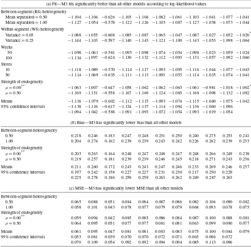
Table1[part (a)] shows the mean log-likelihood values by model type and experimental factor for all factors having signif-icant interactions with model type (for other factors, the pattern of results does not depend on model specification). Model M3 (random coefficients nested logit explaining within-store het-erogeneity using store data) has by far the best fit to the data. In general, the best-fitting models are the ones that allow the most flexible heterogeneity structures. For the random coeffi-cients models, for example, the best-fitting models are the ones that allow heterogeneity across store visits (within-store hetero-geneity), across households, across weeks, and across stores, in that order, coinciding with the number of units allowed to have different sets of parameters. (Similar results are obtained for the finite mixture specifications.) The worst-fitting models are M1 (homogeneous model for store data), M8 (homogeneous model for panel data), and M5 (random coefficients model, across-store heterogeneity), which allow little (in the case of M5) or no (in the case of M1 and M8) heterogeneity in parameters.
The factor-level means in the right-most column of Table1, part (a), generally have the expected patterns. Only within-segment heterogeneity and the strength of endogeneity have statistically significant main effects, the largest of which is for the endogeneity factor. Endogeneity in prices results in signifi-cantly worse fit because random demand shocks correlated with prices are added to the utility function to create the endogeneity condition, and additional randomness always produces worse fit. The end result is an increase in the variance of the error term.
3.2 Analysis of Bias in Sales Response Predictions
We also conducted an ANOVA on the bias in sales response predictions. Simple contrasts show that model M3 (random
Table 1. Simulation results for fit, bias, and MSE
Data factors M1 M2 M3 M4 M5 M6 M7 M8 M9 M10 Means*
(a) Fit—M3 fits significantly better than all other models according to log-likelihood values
Between-segment (BS) heterogeneity
Mean separation=0.50 −1.104 −1.104 −0.626 −1.103 −1.104 −1.082 −1.061 −1.103 −1.041 −1.077 −1.041 Mean separation=1.00 −1.127 −1.054 −0.578 −1.122 −1.126 −1.105 −1.087 −1.127 −1.038 −1.073 −1.044 Within-segment (WS) heterogeneity
Variance=0.05 −1.088 −1.055 −0.608 −1.085 −1.087 −1.065 −1.047 −1.087 −1.027 −1.052 −1.020* Variance=0.25 −1.144 −1.103 −0.597 −1.140 −1.143 −1.121 −1.100 −1.143 −1.053 −1.098 −1.064 Weeks
50 −1.098 −1.061 −0.581 −1.095 −1.098 −1.074 −1.054 −1.098 −1.023 −1.059 −1.024 100 −1.134 −1.097 −0.624 −1.130 −1.132 −1.112 −1.093 −1.131 −1.057 −1.092 −1.060 Stores
10 −1.118 −1.089 −0.570 −1.114 −1.117 −1.093 −1.095 −1.116 −1.044 −1.077 −1.043 50 −1.114 −1.069 −0.635 −1.111 −1.113 −1.093 −1.053 −1.114 −1.035 −1.074 −1.041 Strength of endogeneity
ρ=0.00** −1.063 −1.007 −0.647 −1.058 −1.062 −1.062 −1.063 −1.061 −0.981 −1.018 −1.002* ρ=0.50 −1.169 −1.151 −0.558 −1.167 −1.169 −1.124 −1.085 −1.168 −1.098 −1.132 −1.082
Means −1.116 −1.079 −0.602 −1.112 −1.115 −1.093 −1.074 −1.115 −1.040 −1.075 −1.042 95% confidence intervals −1.138 −1.116 −0.617 −1.134 −1.137 −1.114 −1.094 −1.136 −1.060 −1.096
−1.094 −1.042 −0.588 −1.091 −1.093 −1.072 −1.054 −1.093 −1.019 −1.054
(b) Bias—M3 has significantly lower bias than all other models
Between-segment heterogeneity
0.50 0.218 0.246 0.183 0.247 0.248 0.251 0.250 0.240 0.275 0.253 0.241 1.00 0.204 0.274 0.162 0.239 0.239 0.243 0.242 0.226 0.262 0.239 0.233 Strength of endogeneity
ρ=0.00** 0.203 0.263 0.164 0.248 0.247 0.248 0.247 0.248 0.266 0.249 0.238 ρ=0.50 0.219 0.257 0.181 0.239 0.239 0.246 0.245 0.218 0.271 0.243 0.236
Means 0.211 0.260 0.172 0.243 0.243 0.247 0.246 0.233 0.269 0.246 0.237 95% confidence intervals 0.197 0.242 0.158 0.227 0.227 0.231 0.230 0.217 0.250 0.229
0.225 0.278 0.186 0.259 0.259 0.263 0.262 0.249 0.287 0.263
(c) MSE—M3 has significantly lower MSE than all other models
Between-segment heterogeneity
0.50 0.065 0.088 0.051 0.084 0.084 0.087 0.086 0.082 0.106 0.090 0.082 1.00 0.058 0.101 0.043 0.078 0.077 0.079 0.079 0.068 0.093 0.078 0.075 Strength of endogeneity
ρ=0.00** 0.059 0.094 0.042 0.085 0.085 0.086 0.084 0.087 0.100 0.088 0.081 ρ=0.50 0.064 0.095 0.051 0.077 0.077 0.081 0.081 0.063 0.099 0.080 0.077
Means 0.061 0.095 0.047 0.081 0.081 0.083 0.083 0.075 0.100 0.084 0.079 95% confidence intervals 0.053 0.081 0.039 0.070 0.070 0.072 0.071 0.065 0.086 0.072
0.070 0.109 0.054 0.092 0.092 0.094 0.094 0.085 0.113 0.096
NOTE: Only factors with statistically significant main effects or interactions with model type are shown. * indicates statistically significant main effects for factor; ** is correlation between price and demand equation error terms. Models fitted to store-level data: M1, Homogeneous nested logit; M2, Finite mixture nested logit, within-store heterogeneity; M3, Random coefficients nested logit, within-store heterogeneity; M4, Finite mixture nested logit, across-store heterogeneity; M5, Random coefficients nested logit, across-store heterogeneity; M6, Finite mixture nested logit, temporal heterogeneity; M7, Random coefficients nested logit, temporal heterogeneity. Models fitted to panel data: M8, Homogeneous nested logit; M9, Random coefficients nested logit, across-household heterogeneity; M10, Finite mixture nested logit, across-household heterogeneity.
coefficients nested logit, within-store heterogeneity) produces significantly lower bias than the baseline homogeneous nested logit model applied to store-level data (M1), whereas all other model specifications produce significantlyhigherbias than M1. The number of stores and the number of households per store have significant main effects on bias (increases in both factors produce lower bias, as expected), while between-segment het-erogeneity and strength of endogeneity have significant
interac-tions with model type (but no main effects). Other manipulated factors have no effects on bias.
Table1, part (b) shows the mean bias values by model type and experimental factor for all factors having significant inter-actions with model type (for other factors, the pattern of results does not depend on the model specification). Consistent with the results for fit we find that M3 (random coefficients nested logit, within-store heterogeneity) has significantly lower bias
324 Journal of Business & Economic Statistics, April 2011
in sales response predictions than all other models. Though all other specifications produce significantly higher bias than the homogeneous nested logit applied to store-level data, these dif-ferences across model types are small from a practical stand-point, regardless of the heterogeneity specification and regard-less of the level of data aggregation. M9 (random coefficients nested logit, across-household heterogeneity) and M2 (finite mixture nested logit, within-store heterogeneity) have higher bias values than all other models, which is surprising given the good fit of these models [Table1, part (a)].
Though endogeneity affects model biases in slightly differ-ent ways, resulting in a significant model by endogeneity inter-action, the strength of endogeneity has no significant main ef-fect [note the mean values in the right-most column of Table1, part (b)]. The lack of a significant main effect for endogeneity indicates that the instrumental variables estimation is effective for parameter estimation and generation of sales response pre-dictions, despite its detrimental effect on fit.
3.3 Analysis of Mean Squared Error in Sales Response Predictions
Finally, we conducted a repeated measures ANOVA on the squared sales response prediction errors. The mean squared er-ror (MSE) captures bias and variance in sales response predic-tions and is thus a more comprehensive measure of error. As with the bias measure, M3 produces significantly lower MSE values than the baseline homogeneous logit model applied to store-level data, while all other specifications produce signif-icantly higher MSE values than the homogeneous logit. All MSE results in Table1, part (c) are completely consistent with the bias results in part (b), so we do not discuss these results in detail.
To see how the results of the simulation translate to an actual scanner panel dataset, we estimate all 10 model specifications using scanner panel data from IRI.
4. APPLICATION TO ACTUAL DATA
The panelists for this application, who shopped in nine stores located in a Chicago suburban area, are tracked over the 112-week period from September 1995 to November 1997. A ran-dom sample of 300 households tracked over 52 weeks is used for analysis. The total number of store trips made by the sample panelists during the calibration period was 25,105, with 2022 of the trips resulting in the purchase of paper towels; panelists pur-chased 3499 rolls of paper towels. We focus on single-roll packs in the paper towel category. Brand names with 3% or greater market share were retained for analysis. Price, store feature ad-vertising, and aisle display data are available. The price vari-able is shelf price, inclusive of promotions. We found that, of the two promotional variables, only aisle display was important as a predictor.
To create a measure of promotional response, we use the same general procedure used in the simulation for instituting random price reductions through increases in the promotional depth (0.10–0.25) and frequency (10%–25%), with three differ-ences. First, since we have only one dataset, we simulate new promotion environments for each brand separately, whereas in
the simulation study we randomly selected one brand for analy-sis in each dataset. Second, to control simulation error associ-ated with the generation of the new promotion environments, we generate 300 new promotional environments (replications) for each brand for the one dataset, whereas in the simulation, we generated one new promotional environment for each of 320 datasets. Finally, for the simulation, since the true sales re-sponse predictions were known, we computed bias and MSE criteria to assess the accuracy of the models’ sales response predictions. Since the true sales response predictions are not known with the actual data, we assess the convergence of pre-dictions from different heterogeneity specifications by present-ing the correlations of the models’ sales response predictions across simulated promotional scenarios.
In Table2we show (a) the posterior fit of the various mod-els and (b) the correlations of the modmod-els’ sales response pre-dictions across simulated promotional scenarios. Looking first at model fit, we see that, as was the case with the simulation, M3 fits far better than any other model, with M9 and M2 also fitting better than most other models. Consistent with the simu-lation results, models specified with within-store heterogeneity or across household heterogeneity fit the data best due to their less restrictive assumptions on the nature of heterogeneity.
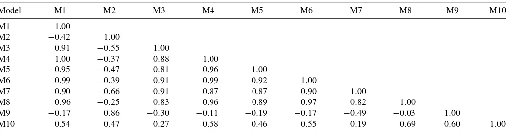
The correlations of sales response predictions across simu-lated scenarios are shown in part (b) of Table2. The conver-gence of predictions from the homogeneous models (M1 and M8) and various store-level specifications (M4, M5, M6, and M7) is generally high and consistent with the findings of the simulation. The predictions of M9 (random coefficients nested logit, across-household heterogeneity) and M2 (finite mixture nested logit, within-store heterogeneity) are not convergent with those of other models, despite the good fit of these mod-els. For M9 (random coefficients nested logit, across-household heterogeneity), the distribution of price coefficients is not cred-ible, with a mean of−6.01 and a standard deviation of 4.19. As a point of reference, the homogeneous models M1 and M8 produce statistically significant price coefficient estimates of
−1.09. The posterior estimates of household-level price coef-ficients from M9 range from−10.53 to 3.95, which is a very wide range for the coefficients and is not very believable. These estimates should serve as warning signals to an analyst that per-haps the model should not be used as a basis for managerial decision making.
Closer inspection of the M2 model estimates shows that the model is poorly identified and unstable. The standard error of one of the brand constants is 502, and in some runs, the co-variance matrix of the parameters even fails to invert. These are clear signals to the analyst that the model should not be used for managerial decision making.
M3 (random coefficients nested logit, within-store hetero-geneity) produces predictions that are reasonably consistent with those of other models. Inspection of the model estimates reveals believable parameters for the distribution of the price coefficients (mean= −2.24, SD=0.32) and promotion coeffi-cients (mean=1.89, SD=0.73). Thus, we have no reason to believe that M3 performs any differently in the empirical appli-cation than it did in the simulation study, given its excellent fit and reasonable parameter estimates.
In conclusion, we observe a general consistency between the analysis of the paper towel category and the simulation results.
Table 2. Empirical application to data from paper towel product category (a) Posterior fit
Model Posterior fit, LL
M3 −0.1610
M9 −0.3054
M10 −0.3614
M2 −0.3655
M5 −0.3929
M4 −0.3996
M7 −0.4002
M6 −0.4071
M1 −0.4100
M8 −0.4100
(b) Correlations of sales response predictions across simulated scenarios
Model M1 M2 M3 M4 M5 M6 M7 M8 M9 M10
M1 1.00
M2 −0.42 1.00
M3 0.91 −0.55 1.00
M4 1.00 −0.37 0.88 1.00
M5 0.95 −0.47 0.81 0.96 1.00
M6 0.99 −0.39 0.91 0.99 0.92 1.00
M7 0.90 −0.66 0.91 0.87 0.87 0.90 1.00
M8 0.96 −0.25 0.83 0.96 0.89 0.97 0.82 1.00
M9 −0.17 0.86 −0.30 −0.11 −0.19 −0.17 −0.49 −0.03 1.00
M10 0.54 0.47 0.27 0.58 0.46 0.55 0.19 0.69 0.60 1.00
NOTE: Models fitted to store-level data: M1, Homogeneous nested logit; M2, Finite mixture nested logit, store heterogeneity; M3, Random coefficients nested logit, within-store heterogeneity; M4, Finite mixture nested logit, across-within-store heterogeneity; M5, Random coefficients nested logit, across-within-store heterogeneity; M6, Finite mixture nested logit, temporal heterogeneity; M7, Random coefficients nested logit, temporal heterogeneity. Models fitted to panel data: M8, Homogeneous nested logit; M9, Random coefficients nested logit, across-household heterogeneity; M10, Finite mixture nested logit, across-household heterogeneity.
The ordering of the models according to fit is generally consis-tent, with M3 having vastly superior fit and M2 and M9 fitting better than most other models. We observe in the empirical ap-plication that M9 and M2 produce sales response predictions that are inconsistent with those of other models; in the simu-lation, we observe that M9 and M2 have the largest biases in sales response predictions as well as the largest MSE. In the empirical application, inspection of the model estimates pro-duces strong signals as to the validity of the predictions.
We do not mean to suggest that M2 and M9 produce such poor results across all empirical applications. The analysis of a single dataset from the paper towel category shows that the idio-syncrasies of any particular dataset can result in very poor out-comes for some models. In contrast, simulation results produce insights into the patterns of model convergence and divergence over a large number of conditions and replications, pointing to most likely outcomes.
5. CONCLUSION
The goal of this study is to explore via simulation whether the sales response predictions from demand models with vari-ous heterogeneity specifications converge or diverge under dif-ferent levels of data aggregation and various heterogeneity con-ditions, endogeneity concon-ditions, and sample size conditions. No prior study has explored the convergence of sales response pre-dictions from a wide variety of models fitted to store and panel
data across a variety of conditions commonly faced by market-ing analysts.
With regard tofit, the study shows that, on average, the flexi-bility of the heterogeneity specification for a demand model has much impact on fit, whereas the level of data aggregation does not. The model with the least restrictive heterogeneity specifica-tion (within-store heterogeneity, which refers to heterogeneity across store visits) fits better than all other models, while ho-mogeneous models assuming parameter invariance across store visits, households, weeks, and stores produced the worst fit. Models with the best fit did not necessarily produce the most ac-curate predictions of sales response to promotions. This is rem-iniscent of findings of other panel data-based simulation studies using different measures of model performance, as well as other empirical studies (e.g., Foekens, Leeflang, and Wittink1994).
With regard to the accuracy of sales response predictions, the simulation shows compelling evidence that sales response pre-dictions are similarly accurate across models, including models applied to panel and store-level data, models explaining hetero-geneity across households, stores, and weeks, and even mod-els explaining no heterogeneity, with one important exception: models explaining within-store heterogeneity (i.e., heterogene-ity across store visits) using random distributions for the coef-ficients produced predictions that were significantly more ac-curate than those of all other models. One implication of this finding is that if the sole objective of the analysis is to predict market response to a new promotional environment, store-level
326 Journal of Business & Economic Statistics, April 2011
data should suffice for such a task. Since store-level data are generally cheaper to obtain, more widely available, and more computationally efficient than panel data, this is an important finding.
We note that, technically, none of the model specifications has a completely correct specification of consumer heterogene-ity since we adopted a mixture of normal distributions for within-market across-consumer heterogeneity, with the mixture components weighted differently for different markets. The ran-dom coefficients within-store specification produces the most accurate sales response predictions because it is capable of cap-turing heterogeneity across store visits, which is a more flexi-ble specification than those used to capture heterogeneity across households, stores, or weeks. The finite mixture version of this specification is not as flexible as the random coefficients version and is, therefore, not as effective. In addition, as was demon-strated in the empirical application, the finite mixture version sometimes produces unstable results.
An empirical application to actual scanner data shows that models producing the least accurate sales response predictions in the simulation also produce divergent sales forecasts in the empirical application, despite good fit statistics. Our analysis indicates that the face validity of model results (e.g., evidence of instability of estimates or lack of identification or unrealistic parameters for coefficient distributions, particularly the distri-butions of price and promotion coefficients) provides a good indication as to whether a model might perform poorly. The idiosyncrasies of any particular dataset can produce very differ-ent outcomes for some models, underscoring the value of the simulation results, which point to most-likely, big-picture out-comes.
Much work remains to be done in the area of logit-based de-mand models. In this study, the specifications of the panel and store-level models are equivalent apart from the heterogeneity specification. One question that arises is how will the conver-gence of predictions between store-level and panel data mod-els be affected if more household-specific constructs such as purchase-event feedback or choice sets were included in the model specification? Such constructs are invariably important predictors of household-level choices, yet they cannot be used for store-level data. We hope that our research will stimulate ongoing research on modeling promotional response with store-level data versus panel data.
SUPPLEMENTAL MATERIALS
Appendices: Appendix A contains the simulation design and procedures. Appendix B contains the models fitted to simu-lated datasets. (Supplemental appendices.pdf)
ACKNOWLEDGMENTS
The authors thank the co-editors, the area editor, and the re-viewers for their very helpful comments on this manuscript.
[Received September 2007. Revised October 2009.]
REFERENCES
Andrews, R. L., and Ebbes, P. (2009), “Properties of Instrumental Variables Estimation in Logit-Based Demand Models: Finite Sample Results,” un-published manuscript, University of Delaware. [321,322]
Andrews, R. L., Ainslie, A., and Currim, I. S. (2002), “An Empirical Compari-son of Logit Choice Models With Discrete versus Continuous Representa-tions of Heterogeneity,”Journal of Marketing Research, 39, 479–487. [320] Berry, S., Levinsohn, J., and Pakes, A. (1995), “Automobile Prices in Market
Equilibrium,”Econometrica, 63, 841–890. [321]
Besanko, D., Dubé, J. P., and Gupta, S. (2003), “Competitive Price Discrimi-nation Strategies in a Vertical Channel Using Aggregate Retail Data,” Man-agement Science, 49, 1121–1138. [319]
Bodapati, A. V., and Gupta, S. (2004), “The Recoverability of Segmentation Structure From Store-Level Aggregate Data,”Journal of Marketing Re-search, 41, 351–364. [319-321]
Bucklin, R. E., Gupta, S., and Siddarth, S. (1998), “Determining Segmenta-tion in Sales Response Across Consumer Purchase Behaviors,”Journal of Marketing Research, 35, 189–197. [320]
Chintagunta, P. K. (2001), “Endogeneity and Heterogeneity in a Probit Demand Model: Estimation Using Aggregate Data,”Marketing Science, 20, 442– 456. [319,320]
Chintagunta, P. K., Dubé, J. P., and Singh, V. (2002), “Market Structure Across Stores: An Application of a Random Coefficients Logit Model With Store Level Data,” inAdvances in Econometrics, eds. P. H. Franses and A. Mont-gomery, Amsterdam, NY: JAI Press. [319]
Foekens, E. W., Leeflang, P. S. H., and Wittink, D. R. (1994), “A Comparison and an Exploration of the Forecasting Accuracy of a Loglinear Model at Different Levels of Aggregation,”International Journal of Forecasting, 10, 245–261. [325]
Gupta, S., Chintagunta, P. K., Kaul, A., and Wittink, D. R. (1996), “Do Household Scanner Panels Provide Representative Inferences From Brand Choices? A Comparison With Store Data,”Journal of Marketing Research, 33, 383–398. [319]
Hoch, S. J., Kim, B. D., Montgomery, A. L., and Rossi, P. E. (1995), “Determi-nants of Store-Level Price Elasticity,”Journal of Marketing Research, 32, 17–29. [319]
Montgomery, A. L. (1997), “Creating Micro-Marketing Pricing Strategies Us-ing Supermarket Scanner Data,”Marketing Science, 16, 315–337. [319] Park, S., and Gupta, S. (2009), “Simulated Maximum Likelihood Estimator for
the Random Coefficient Logit Model Using Aggregate Data,”Journal of Marketing Research, 46 (August), 531–542. [321]
Petrin, A., and Train, K. (2010), “A Control Function Approach to Endogeneity in Consumer Choice Models,”Journal of Marketing Research, 46, 3–13. [321]
Raju, J. S. (1992), “The Effect of Price Promotions on Variability in Product Category Sales,”Marketing Science, 11, 207–220. [320]
Shugan, S. M. (2004), “Endogeneity in Marketing Decision Models,” Market-ing Science, 23, 1–3. [320]
Sudhir, K. (2001), “Competitive Pricing Behavior in the Auto Market: A Struc-tural Analysis,”Marketing Science, 20, 42–60. [319]
Train, K. E. (2003),Discrete Choice Methods With Simulation, Cambridge: Cambridge University Press. [322]
Van Heerde, H. J., Leeflang, P. S. H., and Wittink, D. R. (2000), “The Esti-mation of Pre- and Postpromotion Dips With Store-Level Scanner Data,” Journal of Marketing Research, 37, 383–395. [319]
Villas-Boas, J. M., and Winer, R. S. (1999), “Endogeneity in Brand Choice Models,”Management Science, 45, 1324–1338. [321]