Full Terms & Conditions of access and use can be found at
http://www.tandfonline.com/action/journalInformation?journalCode=ubes20
Download by: [Universitas Maritim Raja Ali Haji] Date: 11 January 2016, At: 23:05
Journal of Business & Economic Statistics
ISSN: 0735-0015 (Print) 1537-2707 (Online) Journal homepage: http://www.tandfonline.com/loi/ubes20
Nonparametric Identification and Estimation in a
Roy Model With Common Nonpecuniary Returns
Patrick Bayer, Shakeeb Khan & Christopher Timmins
To cite this article: Patrick Bayer, Shakeeb Khan & Christopher Timmins (2011) Nonparametric Identification and Estimation in a Roy Model With Common Nonpecuniary Returns, Journal of Business & Economic Statistics, 29:2, 201-215, DOI: 10.1198/jbes.2010.08083
To link to this article: http://dx.doi.org/10.1198/jbes.2010.08083
View supplementary material
Published online: 01 Jan 2012.
Submit your article to this journal
Article views: 205
Nonparametric Identification and Estimation
in a Roy Model With Common
Nonpecuniary Returns
Patrick BAYER
Department of Economics, Duke University, Durham, NC 27708 and NBER (patrick.bayer@duke.edu)
Shakeeb KHAN
Department of Economics, Duke University, Durham, NC 27708 (shakeebk@econ.duke.edu)
Christopher TIMMINS
Department of Economics, Duke University, Durham, NC 27708 and NBER (christopher.timmins@duke.edu)
We consider identification and estimation of a Roy model that includes a common nonpecuniary utility component associated with each choice alternative. This augmented Roy model has broader applications to many polychotomous choice problems in addition to occupational sorting. We develop a pair of non-parametric estimators for this model, derive asymptotics, and illustrate small-sample properties with a series of Monte Carlo experiments. We apply one of these models to migration behavior and analyze the effect of Roy sorting on observed returns to college education. Correcting for Roy sorting bias, the returns to a college degree are cut in half. This article has supplementary material online.
KEY WORDS: Returns to education; Roy model; Sorting.
1. INTRODUCTION
In the original application of his model, Roy (1951) showed that the self-selection of individuals into occupations generally implies that observed wages (conditional on occupation choice) differ markedly from the underlying distribution of wages in the population. The Roy model has subsequently been applied to a wide class of problems in economics, because its structure fits any setting in which individuals choose among a set of alter-natives to maximize an outcome associated with that choice. Given the Roy model’s wide applicability, an important line of recent research has analyzed identification in this model. Be-ginning with Heckman and Honore (1990), this literature has produced a series of results that clarify the conditions under which the underlying population distribution of wages can (or cannot) be identified in observational data.
In this article we study the identification and estimation of a Roy model that includes, in addition to the usual sorting with respect to wage draws, a common nonpecuniary component of utility associated with each alternative that either is constant or depends only on observed variables. An important limitation of the pure Roy model is that it assumes that individuals max-imize only economic returns (e.g., wages). Yet nonpecuniary aspects of decisions are important in many economic applica-tions. In the choice of occupation, for example, nonpecuniary components of utility would include the amenity value or in-jury risk associated with different jobs. In modeling the choice of labor market or residence, the nonpecuniary component of utility would capture variation in amenities and cost of living across cities. This generalized version of the pure Roy model is also applicable to settings in which the outcome of interest is not economic returns. In studying the choice of health behav-iors or medical treatments, the relevant outcome might be the
survival rate, whereas the nonpecuniary component of utility might capture the enjoyment associated with a behavior (such as smoking) or disutility of side effects associated with various treatments. Likewise, in the study of school choice, the relevant outcome might be achievement scores, whereas other factors affecting the choice of school (e.g., availability of special edu-cation programs) might be included as part of a separate com-ponent of utility. In this way, the generalized model developed here can be applied to a wide class of problems in economics.
We provide two distinct sets of conditions under which the nonpecuniary values associated with each choice alternative are nonparametrically identified. Following Heckman and Honore (1990), the identification of the full population wage distribu-tion requires addidistribu-tional identifying assumpdistribu-tions; the key insight of this article is that the nonpecuniary value of alternatives in a generalized Roy model can be identified even in a single cross-section. The emphasis here is on the identification of a particu-lar parameter related to nonpecuniary returns. Thus our identifi-cation comes at the expense of imposing more structure, that is, a sector-specific constant characterizing nonpecuniary returns.
Throughout the article, we consider the nonparametric identi-fication of the model in a relatively demanding setting in which the set of available choices is large and identification at infin-ity is difficult. Identification of this sort of problem has been studied extensively in the literature, especially in the binomial
choice problem (see, e.g., Heckman and Honore1989;
Heck-man 1990). Given the a close link between Roy models and competing-risk models, several of the papers surveyed by Pow-ell (1994) are also related to the models that we explore here.
© 2011American Statistical Association Journal of Business & Economic Statistics April 2011, Vol. 29, No. 2 DOI:10.1198/jbes.2010.08083
201
Some more recent related work includes that of Honore (2002), Lee (2006), Honore and Lleras-Muney (2006), Khan and Tamer (2009), and Lee and Lewbel (2009). Although the identification at infinity strategy can be extended to the multinomial choice setting, the requisite demands on the data are enormous, requir-ing, for example, the availability of distinct combinations of co-variates that compel individuals to select each choice with cer-tainty. The objects to be identified are the population wage dis-tributions and a common nonpecuniary utility associated with each choice. In developing a first set of conditions for identifi-cation, we need only impose the assumption that the distribu-tion of pecuniary returns has a finite lower bound whose value is independent of returns (both pecuniary and nonpecuniary) as-sociated with other choices (i.e., an “extreme quantile indepen-dence” assumption). Given this assumption, we demonstrate that the difference in the minimum order statistic for any two al-ternatives exactly identifies the difference in the nonpecuniary value of those choices. Intuitively, this follows directly from the observation that no individual will choose a less-preferred choice (on the basis of nonpecuniary considerations) unless the wage offered there exceeds this threshold. Thus, the minimum wage observed in the less-preferred sector should be exactly the minimum wage observed in the more-preferred sector plus the difference in nonpecuniary components. Note that within the pure Roy model, the minimum order statistics would be iden-tical for all choices, and the full empirical content of the data would in fact be absorbed by a specification including indepen-dent population wage distributions, as suggested by Heckman and Honore (1990). Having identified the nonpecuniary com-ponent of utility, we show that it is then straightforward to back out underlying unconditional population wage distributions us-ing transformed versions of the observed conditional wages dis-tributions for each sector and the Kaplan–Meier (1958) proce-dure, if independence is assumed, or to apply Petersen (1976) bounds to the transformed data to bound the unconditional pop-ulation wage distribution.
Although this estimator works very well in certain data en-vironments, relying exclusively on differences in minimum or-der statistics to identify the nonpecuniary component of util-ity raises concerns about measurement error. As a result, we consider a second set of formal identifying assumptions. Our second identification proof is based on two key assumptions. First, we assume independence. Following the existing litera-ture, this assumption can be relaxed in more generous data en-vironments (e.g., when data are available for more than a single cross-section or when covariates of the sort used in the literature are available). For example, Khan and Tamer (2009) achieved identification results under strong support conditions in a semi-parametric Roy model. Honore and Llera-Muney (2006) estab-lished set identification when the independence assumption is relaxed.
Second, we assume that information is available for (at least) two subsets of the population that differ in their nonpecuniary valuation of the set of choice alternatives. In the application that we present herein, we consider the choice of regional labor market; in that context, moving costs (broadly defined) natu-rally imply that birth region affects the nonpecuniary value as-cribed to a particular destination. We then exploit the fact that wage offers are likely to be similar for individuals with similar
characteristics from neighboring regions, whereas the nonpe-cuniary value of residing in these regions will vary significantly depending on an individual’s birthplace. We refer to this second assumption as “commonality,” that is, a common wage distrib-ution characterizes wage offers for all individuals regardless of birthplace. In one sense, this commonality assumption can be interpreted as an exclusion assumption; that is, birth location can be regarded as an excluded variable that affects the nonpe-cuniary component of utility but does not affect wages. More-over, this exclusion restriction is easy to use in our empirical context as long as there are more than two locations. Given this assumption, we prove that both the nonpecuniary components of utility for each population subset and the overall population wage distributions are identified.
In this case, some intuition as to why the model is identified by the commonality assumption can again be gained by refer-ring back to the work of Heckman and Honore (1990). Without nonpecuniary components of utility, the observed conditional wage distributions and choice probabilities map uniquely to a set of independent population wage distributions. However, with at least two subsets of the population that have differing nonpecuniary valuations of alternatives, the resulting uncondi-tional wage distributions that would reconcile the two subsets of the data would differ. What our identification proof ensures is that the identical unconditional wage distributions for each subset can be reconciled only at the true values of the nonpecu-niary components of utility for each population subset.
Estimation of this model follows directly from the identifica-tion proof. As we show later, it is possible to write a system of equations based on the observed conditional wage distributions that must equal zero identically at the true values of the nonpe-cuniary parameters for each population subset. These equations serve as natural moments for a minimum distance estimator.
These results add to a sparse literature on the nonparamet-ric identification of a Roy model with numerous alternatives and nonpecuniary components of utility. Dahl (2002) proposed a multinomial version of the estimator developed in the bino-mial context by Ahn and Powell (1993). His extension relies on the key assumption that a nonparametric selection correction term can be based on the first-best choice probability. This as-sumption is not based on a model of utility maximizing behav-ior, however. Other work has examined spatial sorting behavior based on wages and nonpecuniary benefits. Falaris (1987) and Davies, Greenwood, and Li (2001) studied the determinants of migration decisions in Venezuela and the United States, respec-tively. Falaris applied Lee’s (1983) generalized polychotomous choice model to control for nonrandom selection bias in condi-tional wage distributions, whereas Davies et al. essentially ig-nored it. The entire literature on wage hedonics, beginning with Roback (1982), has similarly ignored this problem. In that liter-ature, wage and housing price gradients across cities are used to back out the value of urban amenities. Wage distributions con-ditional on nonrandom selection into cities are typically used to calculate the first of these gradients, leading to biased estimates. We conclude this article by applying our estimator to U.S. Census data to study the effect of spatial sorting on returns to a college education, addressing the same question as considered by Dahl (2002). College graduates are more likely to migrate than are high school graduates, meaning that the bias in their
conditional wage distributions induced by Roy sorting will be greater. Controlling for this bias for both high school and col-lege graduates, we find that the estimated returns to a colcol-lege education at the median fall from 42% to only 18%.
The remainder of the article is organized as follows.
Sec-tion2 introduces the Roy model, proves identification for the
case in which wage distributions are assumed to have a fi-nite lower support that is independent of all wage distributions,
and develops a corresponding estimator. Section3proves
iden-tification under the alternative assumptions of independence and commonality, and develops a corresponding estimator.
Sec-tion4outlines the asymptotic properties of our estimators, and
Section5shows how each estimator performs in finite samples
and under less-than-ideal data circumstances. Section6uses the
second estimator to recover an unbiased estimate of the returns
to a college education. Section7concludes with a discussion of
possible extensions to this research.
2. IDENTIFICATION AND ESTIMATION: FINITE LOWER SUPPORT
We begin our analysis by describing the Roy model with pe-cuniary and nonpepe-cuniary returns. We then prove identification under two separate sets of assumptions. The first case is charac-terized by (a) the assumption that the distribution of the endoge-nously determined payoffs (e.g., wages in a classic Roy model) has a finite lower support, the value of which is independent of (exogenous) wage distributions, and (b) a weaker version of the typical independence assumption used in Roy models. We refer to this assumption as extreme quantile independence and describe it in more detail later.
Our second set of assumptions, which relies on independent wage draws, is applicable in situations where a finite lower sup-port cannot be assumed, or where the minimum order statistic provides a noisy measure of the lower bound. That estimator is
described in detail in Section3. In both cases, we first prove
identification with a simple model describing the sorting of in-dividuals from a single origin location into one of two
destina-tions (k=1,2). We indicate that the wage earned by individual
i, should he choose to settle in locations 1 and 2 asω1,iandω2,i,
respectively. In contrast to the classic Roy model, in which sort-ing is simply across employment sectors and is driven entirely by pecuniary compensation, we model sorting in a geographic context in which the individual’s location decision depends in part on his wage draw in each location, and also on nonwage determinants of utility specific to a particular location, which we call “tastes.” Tastes would certainly include natural ameni-ties and local public goods associated with the destination loca-tion. They also might include costs specific to someone moving from a particular origin to a particular destination. Utility from
choosing to settle in locationkis given by the sum of wages
(ωk,i) and tastes (τk),
Uk,i=ωk,i+τk. (1)
Without loss of generality, we normalizeτ1=0. The goal of
our exercise is to recover estimates ofτ2,f1(ω1), and f2(ω2)
(i.e., the taste parameter associated with location 2 and the un-conditional wage distributions in each location). The difficulty
arises from the fact that we only see wage distributions condi-tional on optimal sorting behavior, and an indicator of which location an individual chooses.
Note that our model is not as flexible as other generalizations of the Roy model found in the literature (e.g., Heckman and
Vytlacil2008) in that we do not allowτk to differ across
indi-viduals. We do this to support our identification strategy, which
allows us to recover thevaluesof taste parameters.
Our first approach uses only the conditional wage
distribu-tions and an indicator of location choice to recoverτ2,f1(ω1),
andf2(ω2)according to the following argument based on
min-imum order statistics. For an individuali, we only observeω2,i
if
ω2,i+τ2≥ω1,i (2)
and we only observeω1,iif
ω2,i+τ2< ω1,i. (3)
Note that Equations (2) and (3) can be regarded as an example
of a generalized Roy model (see Heckman and Vytlacil2008
for a thorough discussion of various generalizations) in which the mechanism for sector selection includes an additive taste pa-rameter that is constant for individuals in a given sector/region. Denote the smallest wage (i.e., the minimum order statistic) that we observe from someone choosing to settle in location 1 by
w1. Definew2similarly. We assume thatf1(ω1)andf2(ω2)have
finite lower points of support (denoted byω∗1 andω∗2,
respec-tively) that are independent of the values ofw1andw2. We refer
to this as an “extreme quantile independence” assumption, anal-ogous to assumption sometimes invoked in the semiparametric literature, where one particular quantile of a random variable is independent of another random variable but all of the other quantiles are allowed to vary. In that sense, we can see that our assumption is weaker than full independence assumption. We
know that the smallest value ofω1that we could ever see given
that individuals maximize utility would be
w1=ω1∗, ifω∗1> ω2∗+τ2,
(4)
w1=ω2∗+τ2, ifω∗1≤ω2∗+τ2.
Similarly, the smallest value ofω2that we could ever see would
be
w2=ω∗2, ifω∗1≤ω∗2+τ2,
(5)
w2=ω∗1−τ2, ifω∗1> ω∗2+τ2.
To make sense of (4) and (5), define the following two cases: A: ω1∗> ω∗2+τ2,
(6)
B: ω1∗≤ω∗2+τ2.
We cannot determine whether case A or B prevails in the data
without recovering an estimate ofτ2. Conveniently, we can
re-cover an estimate ofτ2in either case. In particular,
τ2=w1−w2. (7)
Equation (7) describes our first estimator ofτ2in the simplest
1×2 case. The same logic readily extends to any number of
potential destinations (i.e.,τk=w1−wk,k=1,2, . . . ,K). This
more generalized case is described in the online Appendix.
Having recovered an estimate of τ2, it is a simple matter
to recoverf1(ω1)andf2(ω2)using a variation of the Kaplan–
Meier (1958) procedure typically used in competing-risks mod-els under independence assumptions. Alternatively, we could relax the independence assumption and apply the Petersen (1976) procedure to bound the unconditional distributions. The Kaplan–Meier procedure is described in more detail in the on-line Appendix.
3. IDENTIFICATION AND ESTIMATION: UNBOUNDED SUPPORT
Although the approach described in Section2is clean,
trans-parent, and applicable in certain data environments, using it en-tails two practical problems. First, the payoff variable in ques-tion might not naturally have a finite lower support (e.g., the-ory might dictate using the natural log of wages in the utility function). Second, the minimum order statistic can be a very noisy statistic. Unless one has confidence in the estimate of the minimum order statistic, that noise will be translated directly through to the estimates of the taste parameters and then on to the Kaplan–Meier estimates.
As an alternative approach, we propose in this section an es-timator that uses information from the full distribution of con-ditional wages. Importantly, this approach is valid for an un-bounded support. With that flexibility comes the need for a new identification assumption, however. In particular, we begin by
showing that without such an assumption,τ2,f1(ω1), andf2(ω2)
are not identified. This negative proof reveals just how easily identification can be achieved by exploiting the assumption of
“commonality,” described in Section3.2.
3.1 Nonidentification in the 1×2 Case
We begin with a simple model of individuals sorting over two locations, indexed by 1 and 2. For simplicity, we assume that the individuals are from location 1, and thus we normalize
their taste for staying there to zero (τ1=0). Our interest is in
recovering estimates ofτ2,f1(ω1), andf2(ω2).
We define a variable,di, which functions as an indicator that
individualiremained in his origin location,
di=I[ω1,i> ω2,i+τ2]. (8)
Using this indicator, we can write an expression for individual
i’s observed wage,
wi=diω1,i+(1−di)ω2,i, (9)
that is, the individual receives his draw from location 1 if it was utility-maximizing to remain there. Next, define the following joint probability distributions, both of which are easily observed in the data:
1(t)=P(di=1,wi≤t),
(10)
2(t)=P(di=0,wi≤t).
We also work with the derivatives of these expressions, which we denote by
For this estimator, we need to impose a stronger independence assumption. Rather than assuming only extreme quantile inde-pendence, we assume that all wage draws are independent. We
can then rewrite1(t)as
nipulation, we arrive at the following expression, which
de-scribes the distribution ofω1,ias a function ofτ2:
whereλ1(t)is a function of the unconditional wage
distribu-tion in locadistribu-tion 1. Equadistribu-tion (13) is a single equadistribu-tion in two
unknowns,λ1(t)and τ2, for a particular value oft, and thus
it is not surprising that we cannot identify both of these values without making an additional assumption. One approach to this
would involve making a parametric assumption aboutF1(t);
an-other would be to introduce an exclusion restriction into the model. To illustrate this, assume the presence of an additional
observable variable,z, in Equation (15). Ifztook two values,
say 0 and 1, then for each value, we would have an equation like (25), thus introducing the additional equation needed for identification of the two unknown parameters.
In the next section, we expand on this idea by showing how the assumption of commonality can be used to
nonparametri-cally recoverλ1(t)andτ2. This assumption is analogous to the
sort of exclusion restriction just described—in particular, birth location is a variable that affects the location decision but is assumed to be excluded from the determinants of wages.
We conclude this section by commenting on our nondegen-eracy assumption on the unknown taste parameter. Such an as-sumption is not new to the econonometrics literature and is similar to the structure imposed in threshold regression
mod-els (see, e.g., Hansen2000). Such an approach has been very
popular in time series and now being imposed in
microecono-metric models (see, e.g., Lee and Seo2008). We encountered
some difficulty in attaining identification if we relaxed this as-sumption on the taste parameter. Consequently, identification of the marginal distributions of wages requires a regressor that takes large values [i.e., “identification at infinity” (Heckman
and Vytlacil2008) or, alternatively, “independence at infinity”
(d’Haultfoeuille and Maurel2010)]. Either of these approaches
can result in identification being “irregular” in the sense that rates of convergence of estimators can be slow and can depend on relative tail conditions of the variables in the model, making
inference more complicated. As we show in Section4, this is in
contrast to the properties of our proposed minimum distance es-timator of the taste parameter, which (under our restrictions of common nonpecuniary return and independence) converges at the parametric rate (as does the estimator of the unconditional wage distributions).
3.2 Identification via Commonality in the 2×2 Case
Consider the case of individuals born into one of two loca-tions (again indexed by 1 and 2), who decide where to reside based on the maximization of utility. This introduces the need for additional notation; we use a superscript to indicate origin location and a subscript to indicate destination location.
The dummy variable indicating that an individual originating in location 1 chooses to stay in that location is given by
d1i =I[ω11,i> ω12,i+τ21], (14) whereas the indicator that an individual originating in location 2 chooses not to migrate is given by
di2=I[ω22,i> ω21,i+τ12]. (15) As before, we normalize the taste parameter for those choosing
not to migrate to zero (i.e.,τ11=τ22=0). With these indicators,
we can now write the expression for the observed wage of an
individualiwho originates in location 1,
w1i =di1ω11,i+(1−d1i)ω12,i. (16)
Based on these definitions fordandw, we define the following
expressions analogously to the previous section:
11(t)=P(d1i =1,w1i ≤t), 21(t)=P(d1i =0,w1i ≤t),
(17)
12(t)=P(d2i =0,w2i ≤t), 22(t)=P(d2i =1,w2i ≤t).
Continuing in a manner similar to the previous section, we can use Equation (17) to derive the following four expressions:
λ11(t)= f
nothing to help with identification. It does, however, allow us to introduce an additional assumption: commonality. Under the
assumption of commonality,λ11(t)=λ21(t)andλ12(t)=λ22(t)∀t.
Under this assumption, we can rewrite Equations (18)–(21) as the following two equations:
Estimation proceeds by forming minimum distance criterion functions based on Equations (22) and (23),
λ11(t;τ21)−λ21(t;τ12)=0 (24) and
λ12(t;τ21)−λ22(t;τ12)=0, (25) and then relying on the properties of M-estimators to recover
τ21 and τ12. We then use these taste parameters along with a
Kaplan–Meier procedure to recover estimates of f1(ω1) and
f2(ω2)as described in Section2.
We now provide sufficient conditions for identification and
estimation of the taste parameters in the 2×2 setting with
com-monality. We begin by rearranging Equations (22) and (23) as
21(t−τ21)ψ12(t)−ψ11(t)22(t+τ12) Note that the right side of each expression is an observable
function of the data for a particular value oft. Our identification
result begins with the following lemma.
Lemma 1. At the true parameter values (τ21∗, τ12∗), we have
This is simply a restatement of our minimum distance crite-rion function described above. We now show that for each set of
values of the taste parameters different from (τ21∗, τ12∗), denoted
by the monotonicity of the conditional cumulative distribution functions that make up that expression. By a similar argument,
ifτ˜12=τ12∗, thenτ˜21=τ21∗for Equation (28) to hold. Therefore,
we need only consider the case in whichτ˜21 =τ21∗andτ˜12 =τ12∗.
Is it possible that an imposter pair (τ˜21,τ˜12)could satisfy
Equa-tion (28)?
Consider the following condition, which we argue will be sufficient to rule out this possibility:
ψ21(t−τ21∗)ψ12(t)ψ21(t)ψ12(t−τ12∗)
=ψ11(t+τ21∗)ψ22(t)ψ11(t)ψ22(t+τ12∗) (30)
for some t∈ ℜ in the intersection of the supports of ψ11(t),
ψ21(t), ψ12(t), andψ22(t). This condition has a simple
interpreta-tion—that the Jacobian matrix associated with Equations (26) and (27) is nonsingular. There are situations in which this con-dition will not hold, for example, when the two concon-ditional
wage distributions are identical andτ21= −τ12. This would be
the case if we took a single location and arbitrarily divided it into two locations with the exact same wage distributions and amenities. Thus this condition places a practical constraint on the level of geographic precision at which we can apply our esti-mator, that is, the level at which we can observe different spatial wage distributions. We consider this a pathological case.
To establish the sufficiency of the foregoing condition for identification, consider a local linearization of Equations (26)
and (27) around the true values ofτ21 andτ12and evaluated at
t. For any pair of perturbations,12and21, we require the net
effect on the left side of each equation to be zero, becauseH(t)
andJ(t)are functions only oft:
ψ21(t−τ21∗)ψ12(t)12+ψ11(t)ψ22(t+τ12∗)21=0, (31)
ψ11(t+τ21∗)ψ22(t)12−ψ21(t)ψ12(t−τ12∗)21=0. (32) If condition (30) holds, then the only solution to these
expres-sions is given by12=21=0, implying that no imposter
val-ues of (τ˜21,τ˜12)could satisfy the system. Note that everything
we have here is for a givent. Thus by varying values oftover
values in the intersection of the supports ofψ11(t), ψ21(t), ψ12(t),
andψ22(t), Equations (31) and (32) overidentify the parameters
of interest under our assumptions of independence and com-monality. Consequently, a test for commonality possibly could be based on how far the value of our minimum distance ob-jective function is from zero, loosely analogous to obob-jective function-based specification tests in the generalized method of moments and M-estimation literature.
4. ASYMPTOTICS
Having described two identification strategies for both the taste parameters and unconditional wage distributions, we now outline the arguments that we use in developing the asymptotic properties of our proposed estimators. We begin with a discus-sion of our minimum order statistic estimator. In practice, we simply replace population extreme quantiles in the identifica-tion argument with sample minimum order statistics. Asymp-totic properties of minimum or maximum order statistics have been studied in recent work by Porter and Hirano (2003). Cher-nozhukov and Hong (2004) obtained similar results. As a pre-liminary step, we establish the rate of convergence of the es-timator. The result is based on the following regularity condi-tions:
Assumption A1. The K+1 vectors of observed wage and
choice indicators (wi,dk,i) are iid across individuals.
Assumption A2. The unconditional wage distributions for
al-ternativesk=1,2, . . . ,Kare continuously distributed with
pos-itive density on [ℓk,∞).
Assumption A3. mink=1,2,...,Kℓk>−∞.
Assumption A4. mink=1,2,...,KP(dk,i=1) >0.
Theorem 1. Under AssumptionsA1–A4, we have
ˆ
τk−τk=Op(n−1). (33)
A proof that our estimator attains this rate of convergence
under AssumptionA2follows from arguments similar to those
used by van der Vaart (1998, sec. 21.4).
Turning attention to the second-stage estimator of the uncon-ditional wage distributions, we propose applying Kaplan–Meier
to yield a consistent estimator of the distribution ofωk,I+τk.
We note the first-stage estimator, which was shown to be “su-per consistent,” will have no effect on the limiting distribution of the second-stage estimator. The next theorem establishes the limiting distribution of this estimator.
Theorem 2. Under Assumptions A1–A4, our second-stage estimator of the unconditional wage distribution has the
follow-ing linear representation. Letπ(t)=P(ωk,i≤t)and define the
A proof of the foregoing theorem can be obtained using the same arguments as out forth by in Fleming and Harrington (1991). We omit the details here.
We now turn our attention to the asymptotic properties of the unbounded support estimator. To illustrate the basic arguments involved, we focus on the two-region setting. Our estimator of
the taste parameter vector,τˆ=(τˆ21,τˆ12), is obtained by
mini-mizing the minimum distance objective function,
ˆ
The asymptotic properties of our unbounded support estimator are based on the following assumptions:
Assumption B1. The K+1 vectors of observed wage and
choice indicators (wi,djk,i) are iid across individuals.
Assumption B2. The true vectorτ0 lies in the interior of a compact parameter space.
Assumption B3. The functions ψml(·), l,m=1,2, are as-sumed to be uniformly bounded and twice continuously differ-entiable, with uniformly bounded first and second derivatives.
Assumption B4. The kernel function K(·) used to
approx-imate ψml(·) has bounded support, integrates to 1, and has
mean 0.
Assumption B5. The bandwidth h associated with kernel
functionK(·)satisfies√nh2→0 andnh→ ∞.
Theorem 3. Under AssumptionsB1–B4,
ˆ
τ −→p τ0. (36)
The proof of this result can be obtained by establishing the four sufficient conditions in theorem 2.1 of Newey and McFad-den (1994), which can be characterized as compactness, iMcFad-denti- identi-fication, uniform convergence, and continuity.
Furthermore, by theorem 8.11 of Newey and McFadden (1994), we can establish the parametric rate of convergence as well as the asymptotic normality of our estimator. The paramet-ric rate is attainable despite the nonparametparamet-ric rate of conver-gence achieved by some components, because the parameter of
interest (τ0) is a smooth functional of the nonparametric
compo-nents. Our next theorem is based on the following assumptions:
Assumption B6. The functionsψml,l,m=1,2 are assumed
to be uniformly bounded and p times continuously
differen-tiable, with uniformly boundedpth-order derivatives.
Assumption B7. The kernel function K integrates to 1, has
mean 0, and is ofpth order.
Assumption B8. The bandwidthhassociated with the kernel
function satisfies√nhp→0 andnh→ ∞.
The following theorem establishes the root-nconsistency and
asymptotic normality of our estimator. Its proof is omitted be-cause it follows from the same arguments used in proving the-orem 8.11 of Newey and McFadden (1994).
Theorem 4. Under AssumptionsB1,B2, andB4–B8,
√
n(τ−τ0)⇒N(0, x), (37)
wherexis invertible.
Remark 1. The exact form ofx is complicated, because it
involves higher-order derivatives of the functionsψml. The
de-tails of its form in the 2×2 case, as well as a sketch of the proof
of the theorem, are provided in the online Appendix. Because of its complicated form, we use sampling methods for
infer-ence onτ0 in our application to avoid introducing additional
nonparametric methods.
Remark 2. Note that in this case, the first-stage estimator converges at the parametric rate, and consequently will affect the limiting distribution of the second-stage estimator. Whereas the precise effect on the limiting distribution can be derived us-ing arguments similar to those used by Newey and McFadden (1994, sec. 8), we omit the details here.
5. MONTE CARLO RESULTS
In this section we use Monte Carlo experiments to describe the properties of both estimators in small samples and with less-than-ideal data. We consider a simple setting with just three locations that serve as both origins and destinations, and we model the sorting decisions of individuals who care about both pecuniary returns (i.e., wages) and nonpecuniary factors (i.e., migration costs and amenities) in deciding where to live. In each experiment, we consider some number of identical
indi-viduals (N) originating in each location, and we use their
simu-lated behavior to recover the matrix of taste parameters:
⎡
For the sake of simplicity in exposition, we focus our attention on the performance of the estimators in recovering these taste parameters. Unconditional wage distributions in each location could be recovered by applying the Kaplan–Meier technique
described in Section2for each set of Monte Carlo estimates.
We begin by looking at the minimum order statistic estima-tor. The results of nine Monte Carlo experiments are described
in Table1. The first three experiments use the baseline
frame-work in which wages are random variables determined by the
following (jdenotes origin location):
ωj1=
Columns describe the various taste parameter estimates, and rows summarize the mean, standard deviation, and mean squared error of 500 Monte Carlo simulations for each experi-ment.
With an increasing number of individuals in each origin lo-cation, the minimum order statistic becomes a better measure of the true lower bound on wages in a particular location, and our estimates of the taste parameters improve accordingly. This
is evident in the declining MSE asN increases from 1000 to
10,000 to 50,000 for each parameter. Even with as few as 1000 observations, however, taste parameter estimates based on the minimum order statistic are quite precise.
The fourth and fifth experiments in Table1relax the
assump-tion of a finite lower bound for the uncondiassump-tional wage distrib-ution. In particular,
f(ωj1)∼N(2.25,0.5),
f(ωj2)∼N(1.75,0.5), (40)
f(ωj3)∼N(2.75,0.5),
wherej again denotes the origin location. The impact of this
model misspecification is evident in an increase in the MSE by a factor of 100 to 10,000, depending on the parameter.
Condi-tional on this misspecification, however, MSEs still fall as N
increases from 10,000 to 50,000.
The sixth and seventh experiments address an important con-cern with our minimum order statistic estimator: measurement error. Because the estimator relies on a single value of wages for each origin and destination combination, it could become severely biased if that value were mismeasured. In these exper-iments, we return to the same wage distributions used in the first three experiments (i.e., assuming a finite lower bound), but we add to each wage an iid normally distributed random variable with mean 0 and variance equal to 0.25. This has a significant impact on the precision of our estimates, raising the MSEs as-sociated with our taste parameters by nearly as much as the absence of a finite lower bound. In contrast to that model mis-specification, however, this is primarily the result of an increase in the bias of our estimator, as opposed to its standard deviation.
Table 1. Monte Carlo simulations. Minimum order statistic estimator
τ21 τ31 τ12 τ32 τ13 τ23
−0.5 −0.2 −0.4 −0.6 −0.3 −0.1
1.Baseline(N=1000)
Mean −0.542 −0.203 −0.408 −0.610 −0.316 −0.113 Std. dev. 0.031 0.002 0.006 0.007 0.011 0.009 MSE 0.003 1.28×10⁻⁵ 1.03×10⁻⁴ 1.53×10⁻⁴ 3.63×10⁻⁴ 2.50×10⁻⁴
2.Baseline(N=10,000)
Mean −0.510 −0.201 −0.402 −0.602 −0.303 −0.103 Std. dev. 0.007 4.06×10⁻⁴ 0.001 0.001 0.002 0.002 MSE 1.40×10⁻⁴ 5.36×10⁻⁷ 4.68×10⁻⁶ 7.26×10⁻⁶ 1.71×10⁻⁵ 1.23×10⁻⁵
3.Baseline(N=50,000)
Mean −0.503 −0.200 −0.400 −0.600 −0.301 −0.101 Std. dev. 0.002 1.45×10⁻⁴ 4.19×10⁻⁴ 5.00×10⁻⁴ 7.70×10⁻⁴ 6.51×10⁻⁴ MSE 1.79×10⁻⁵ 6.63×10⁻⁸ 5.54×10⁻⁷ 8.12×10⁻⁷ 2.02×10⁻⁶ 1.33×10⁻⁶
4.Unbounded support(N=10,000)
Mean −0.595 −0.173 −0.389 −0.564 −0.350 −0.184 Std. dev. 0.202 0.212 0.204 0.198 0.215 0.208 MSE 0.050 0.046 0.042 0.040 0.048 0.050
5.Unbounded support(N=50,000)
Mean −0.569 −0.177 −0.383 −0.572 −0.354 −0.161 Std. dev. 0.193 0.189 0.202 0.187 0.183 0.199 MSE 0.042 0.036 0.041 0.036 0.036 0.043
6.Measurement error(N=10,000)
Mean −0.668 −0.248 −0.502 −0.711 −0.439 −0.228 Std. dev. 0.062 0.048 0.050 0.055 0.057 0.056 MSE 0.032 0.005 0.013 0.015 0.023 0.020
7.Measurement error(N=50,000)
Mean −0.660 −0.248 −0.491 −0.697 −0.430 −0.223 Std. dev. 0.050 0.043 0.044 0.044 0.046 0.047 MSE 0.028 0.004 0.010 0.011 0.019 0.017
8.Correlated wage draws(N=10,000)
Mean −0.516 −0.201 −0.402 −0.603 −0.305 −0.104 Std. dev. 0.011 3.89×10⁻⁴ 0.001 0.002 0.003 0.002 MSE 3.78×10⁻⁴ 4.61×10⁻⁷ 5.38×10⁻⁶ 9.76×10⁻⁶ 2.96×10⁻⁵ 1.97×10⁻⁵
9.Correlated wage draws(N=50,000)
Mean −0.506 −0.200 −0.401 −0.601 −0.302 −0.101 Std. dev. 0.004 1.40×10⁻⁴ 4.68×10⁻⁴ 5.76×10⁻⁴ 0.001 7.84×10⁻⁴ MSE 4.83×10⁻⁵ 5.54×10⁻⁸ 6.87×10⁻⁷ 1.02×10⁻⁶ 3.41×10⁻⁶ 2.12×10⁻⁶
In the eighth and ninth experiments, we demonstrate a desir-able feature of the minimum order statistic estimator—the fact that it is robust to arbitrary forms of correlation in wage draws. Using the same wage distributions as in our baseline specifi-cations, we assume a correlation of 0.25 between wage draws in all locations. As is evident from the table, taste parameter estimates are virtually identical to the baseline case.
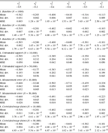
Table 2 describes the results of nine Monte Carlo
experi-ments that similarly illustrate the properties of our unbounded support estimator. Using the same matrix of taste parameters, we assume in our baseline experiment that wages are drawn from the same distributions as described in Equation (40). The first three experiments demonstrate the effect of increasing the
number of individuals originating from each location (N) from
1000 to 50,000. MSEs of all taste parameter estimates fall with an increase in the sample size. In general, however, results are not as precise as under the (properly specified) minimum order
statistic estimator (conditional onN).
In the next two experiments, we show the implications of vi-olating our key identifying assumption—commonality. In par-ticular, we allow nonmigrants to receive a higher wage on av-erage than individuals migrating into their birth location (i.e., a “home advantage” in the labor market):
f(ωj1)∼N(2.25,0.5) ifj=2,3
f(ω11)∼N(2.5,0.5) otherwise,
f(ωj2)∼N(1.75,0.5) ifj=1,3
f(ω22)∼N(2,0.5) otherwise, (41)
f(ωj3)∼N(2.75,0.5) ifj=1,2
f(ω33)∼N(3,0.5) otherwise.
We assume, moreover, that the researcher properly identifies this home advantage and uses only moments formed between
Table 2. Monte Carlo simulations. Unbounded support estimator
τ21 τ31 τ12 τ32 τ13 τ23 −0.5 −0.2 −0.4 −0.6 −0.3 −0.1
1.Baseline(N=1000)
Mean −0.731 −0.230 −0.441 −0.652 −0.404 −0.173 Std. dev. 0.444 0.332 0.422 0.544 0.323 0.156 MSE 0.250 0.111 0.180 0.298 0.115 0.029
2.Baseline(N=10,000)
Mean −0.620 −0.199 −0.390 −0.584 −0.373 −0.171 Std. dev. 0.079 0.066 0.081 0.063 0.053 0.057 MSE 0.021 0.004 0.007 0.004 0.008 0.008
3.Baseline(N=50,000)
Mean −0.614 −0.197 −0.381 −0.573 −0.375 −0.181 Std. dev. 0.047 0.033 0.043 0.032 0.029 0.042 MSE 0.015 0.001 0.002 0.002 0.006 0.008
4.Unbounded support(N=10,000)
Mean −0.576 0.175 −0.103 −0.218 −0.290 −0.303 Std. dev. 0.163 0.415 0.347 0.460 0.133 0.269 MSE 0.032 0.313 0.208 0.358 0.018 0.114
5.Home advantage(N=50,000)
Mean −0.510 −0.101 −0.309 −0.426 −0.354 −0.193 Std. dev. 0.073 0.204 0.156 0.157 0.112 0.128 MSE 0.005 0.078 0.032 0.055 0.015 0.025
6.Correlated wage draws(N=10,000)
Mean −1.362 −0.441 −0.959 −1.367 −0.814 −0.356 Std. dev. 0.487 0.322 0.625 1.032 0.657 0.176 MSE 0.980 0.162 0.702 1.652 0.696 0.096
7.Correlated wage draws(N=50,000)
Mean −1.368 −0.419 −0.950 −1.268 −0.706 −0.421 Std. dev. 0.290 0.057 0.155 0.107 0.171 0.135 MSE 0.838 0.051 0.327 0.458 0.194 0.121
8.Measurement error(N=10,000)
Mean −0.643 −0.206 −0.401 −0.601 −0.382 −0.176 Std. dev. 0.077 0.068 0.083 0.066 0.055 0.060 MSE 0.026 0.005 0.007 0.004 0.010 0.009
9.Measurement error(N=50,000)
Mean −0.632 −0.202 −0.395 −0.592 −0.385 −0.187 Std. dev. 0.052 0.035 0.046 0.034 0.029 0.042 MSE 0.020 0.001 0.002 0.001 0.008 0.009
pairs of migrant groups (e.g., migrants from locations 2 and 3 living in location 1) in forming our minimum distance objec-tive function. Not surprisingly, with this limited set of moments the model does not perform as well as in the baseline specifi-cation. It does, however, do a reasonable job of estimating all parameters (even with only 10,000 observations per origin
lo-cation). WhenNis set equal to 50,000, the estimates become
quite precise, indicating that our estimation strategy is indeed valid under situations of “limited commonality.”
The sixth and seventh experiments describe what happens when another key assumption used in the derivation of the un-bounded support estimator—independence—is violated. Recall that in the derivation of Equation (12), we assumed individu-als received draws from independent wage distributions. Here we assume that wage draws exhibit a positive correlation (0.25) across locations. MSEs for all taste parameters rise dramati-cally, highlighting this as an important shortcoming of our un-bounded support estimation strategy. Whereas this shortcoming
might be addressed with the use of panel data, the current ap-plication use only cross-sectional data, highlighting the impor-tance of controlling for as many forms of observable hetero-geneity as possible (i.e., wages may be systematically higher for certain groups, for which the estimation algorithm should be run separately). Our final set of experiments describes the effect of measurement error on our unbounded support estimator. As was the case for the minimum support estimator, we simply add to each wage an iid normal measurement error with mean 0 and variance 0.25. In contrast to the minimum order statistic esti-mator, however, the results of the unbounded support estimator are affected very little.
In summary, Monte Carlo simulations suggest that our min-imum order statistic estimator performs extremely well when properly specified. It also is robust to arbitrary forms of correla-tion in an individual’s wage draws, but it performs very poorly when wages are observed with error or when they are drawn from a distribution without a finite lower bound. These fail-ures motivate our derivation of the unbounded support estima-tor. When properly specified, experiments show that it also per-forms well. Moreover, its performance is not adversely affected by measurement error in wages or by limited commonality (if the researcher properly recognizes this in forming the minimum distance objective function). In contrast to the minimum or-der statistic estimator, however, it performs poorly when wage draws are correlated across locations.
6. EMPIRICAL APPLICATION: MEASURING THE RETURNS TO COLLEGE EDUCATION
To demonstrate the performance of our estimator in an em-pirical setting, we examine a question similar to that posed by Dahl (2002): What are the returns to a college education (rel-ative to graduating from high school) before and after control-ling for the nonrandom spatial sorting of workers across the United States? The results of the basic Roy model (1951) sug-gest that sorting shifts the means of the (observed) conditional wage distributions up from their (unobserved) unconditional values. Whether spatial sorting increases or reduces the esti-mated returns to a college education will depend on whether this shift is proportionally bigger for high school or college-educated individuals. If, for example, college-college-educated individ-uals were more mobile and thus more able to migrate in re-sponse to favorable idiosyncratic wage draws, we would expect spatial sorting to create an upward bias in the estimated returns to a college education. Whether or not this is the case (and how big is the resulting bias) is an empirical question.
To answer that question, we use data extracted from the 2000
U.S. Census 5% microsample, available fromwww.ipums.org.
Specifically, we consider a sample of 470,918 high school grad-uates taken from each of nine divisions of the United States used by the Census Bureau, along with a corresponding sam-ple of 429,584 college graduates. We use only data describing male household heads because we assume they are more likely to have made their own geographic location decision. We also restrict the sample to individuals under 35 years of age as they are more likely to have recently migrated. Older individuals may have migrated further in the past in response to different wage or amenity distributions. For each individual, we observe
Table 3. Mobility matrix, high school graduates. 2000 U.S. Census, 5% IPUMS random sample
Destination region
New Mid- E. North W. North South E. South W. South
Birth region England Atlantic Central Central Atlantic Central Central Mountain Pacific New England 0.806 0.035 0.011 0.005 0.083 0.008 0.012 0.017 0.024 Mid-Atlantic 0.016 0.809 0.011 0.005 0.100 0.008 0.012 0.019 0.020 E. North Central 0.004 0.013 0.766 0.024 0.072 0.034 0.026 0.031 0.031 W. North Central 0.002 0.006 0.053 0.770 0.028 0.011 0.034 0.053 0.043 South Atlantic 0.008 0.036 0.016 0.007 0.863 0.029 0.017 0.010 0.015 E. South Central 0.003 0.009 0.065 0.009 0.082 0.776 0.032 0.008 0.015 W. South Central 0.002 0.007 0.022 0.025 0.035 0.022 0.814 0.030 0.043 Mountain 0.004 0.009 0.017 0.032 0.027 0.010 0.049 0.747 0.105 Pacific 0.006 0.011 0.021 0.027 0.035 0.012 0.040 0.097 0.750
annual income from wages and salary, the individual’s region of residence, and the individual’s region of birth. We drop any in-dividuals reporting zero annual income, self-employed individ-uals, individuals not born in the United States, and individuals who worked fewer than 45 weeks in the previous year. The U.S. Census describes the individual’s birth state as well as the state in which he or she was living 5 years earlier. We use birth state to define our measure of “origin location,” but a similar analysis could be performed using location 5 years earlier as the
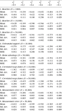
“ori-gin,” leading to a short-run measure of mobility cost. Tables3
and4summarize the long-run migration probabilities observed
in the data for high school and college graduates, respectively, for each of four summary birth and destination locations. In par-ticular, each row indicates the birth location, and each column indicates the location in which the individual is observed in the 2000 Census. Each entry describes the fraction of individuals originating in the row birth location found to be living in the column destination location. As shown, 80.6% of high-school graduates born in New England are found to be living in New England. The fraction of high school graduate “stayers” is sim-ilarly high for other regions. For college graduates, a notably lower percentage remain tied to their respective birth regions.
Because Census wage data, which are derived from self-reported income and hour worked information, are quite noisy in the lower tail (e.g., approximately 3% of individuals report
an implausibly low wage, below 50 ¢/hour), and because we
see individuals from multiple birthplaces, we opt for our
un-bounded support estimator. This estimator makes an indepen-dence assumption and assumes that individuals from different birth regions will receive wage draws from a common destina-tion wage distribudestina-tion. Note that with different data, the extreme quantile estimator (which assumes extreme quantile indepen-dence and wage distributions with a finite lower bound) might be used instead. Deleire, Khan, and Timmins (2009) used this estimator, along with CPS wage data, to recover an estimate of the value of a statistical life (VSL) controlling for Roy sorting across occupations.
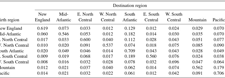
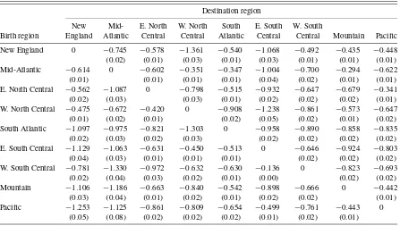
Tables 5 and 6 report the estimates of the taste
parame-ters for high school and college graduates, respectively. Re-sults are measured in terms of the natural log of hourly wages, standard errors are derived from the results of 750 bootstrap simulations, and point estimates are bias-corrected. For exam-ple, a college graduate from the mid-Atlantic region faces a
statistically significant cost of−0.622 per year from moving
to the Pacific region. Considering the mean wage among all
college graduates ($26.22/hour), this amounts to a
compen-sating variation (defined implicitly according to ln(26.22)=
ln(26.22+CV)−0.622)of $22.62/hour. All off-diagonal taste
parameters are negative and significant, demonstrating the ten-dency for individuals of all levels of education to remain in their birth regions.
We next use these estimates to recover the unconditional in-come distributions for each region and education group with the
Kaplan–Meier procedure described in Section2. Results are
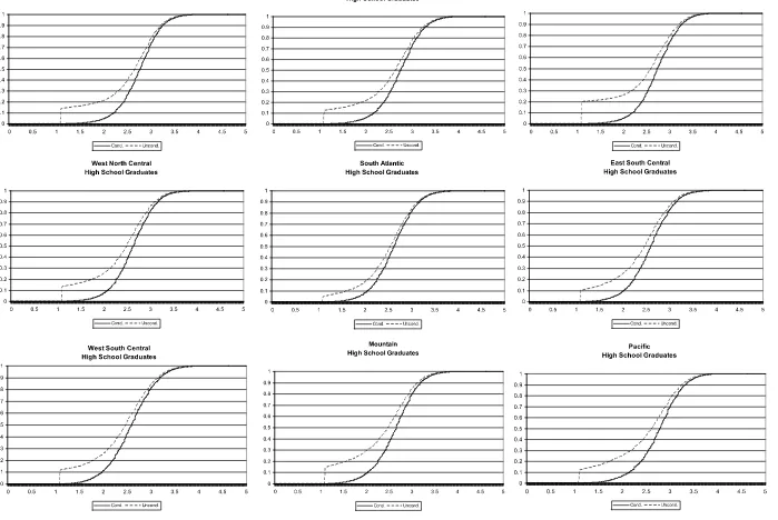
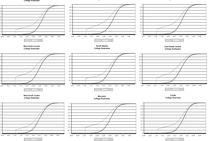
re-ported in Figures1and2. In every case, the unconditional wage
Table 4. Mobility matrix, college graduates. 2000 U.S. Census, 5% IPUMS random sample
Destination region
New Mid- E. North W. North South E. South W. South
Birth region England Atlantic Central Central Atlantic Central Central Mountain Pacific New England 0.619 0.073 0.033 0.012 0.129 0.012 0.024 0.029 0.070 Mid-Atlantic 0.060 0.546 0.053 0.012 0.182 0.014 0.030 0.035 0.070 E. North Central 0.017 0.033 0.600 0.040 0.112 0.028 0.043 0.051 0.077 W. North Central 0.010 0.020 0.091 0.537 0.074 0.018 0.075 0.085 0.090 South Atlantic 0.020 0.049 0.046 0.014 0.709 0.043 0.043 0.028 0.049 E. South Central 0.009 0.019 0.068 0.017 0.189 0.560 0.076 0.024 0.038 W. South Central 0.008 0.016 0.032 0.028 0.078 0.032 0.696 0.047 0.064 Mountain 0.012 0.021 0.037 0.040 0.062 0.014 0.074 0.562 0.179 Pacific 0.014 0.021 0.032 0.022 0.061 0.012 0.042 0.091 0.706
Table 5. Taste parameter estimates. High school graduates
Destination region
New Mid- E. North W. North South E. South W. South
Birth region England Atlantic Central Central Atlantic Central Central Mountain Pacific New England 0 −0.863 −0.562 −0.899 −0.967 −0.972 −0.865 −0.686 −0.948 (0.05) (0.05) (0.15) (0.06) (0.10) (0.08) (0.05) (0.08) Mid-Atlantic −0.803 0 −0.877 −1.092 −0.902 −0.988 −0.921 −0.324 −0.976 (0.06) (0.08) (0.13) (0.05) (0.09) (0.08) (0.03) (0.09) E. North Central −1.036 −0.895 0 −0.960 −1.203 −1.055 −1.011 −0.685 −1.211 (0.17) (0.18) (0.12) (0.08) (0.08) (0.07) (0.06) (0.10) W. North Central −0.390 −0.823 −0.631 0 −1.119 −0.830 −0.815 −0.788 −0.899 (0.05) (0.07) (0.06) (0.11) (0.13) (0.10) (0.05) (0.09) South Atlantic −0.847 −0.742 −0.727 −1.069 0 −0.704 −0.808 −0.801 −0.528 (0.08) (0.08) (0.05) (0.09) (0.06) (0.06) (0.07) (0.08) E. South Central −0.405 −0.585 −0.445 −0.433 −0.874 0 −0.816 −0.995 −0.932 (0.04) (0.04) (0.06) (0.03) (0.07) (0.06) (0.09) (0.17) W. South Central −0.763 −1.231 −0.682 −1.009 −1.108 −0.969 0 −0.699 −1.075 (0.08) (0.15) (0.09) (0.09) (0.09) (0.08) (0.07) (0.08) Mountain −0.878 −0.555 −0.644 −0.774 −0.952 −0.774 −0.859 0 −0.784 (0.15) (0.05) (0.05) (0.10) (0.07) (0.11) (0.06) (0.05) Pacific −0.710 −0.804 −0.550 −0.806 −0.775 −0.994 −0.648 −0.305 0
(0.18) (0.07) (0.05) (0.06) (0.06) (0.10) (0.05) (0.03)
distribution lies below the observed distribution. Importantly, the correction for Roy sorting is generally larger for college graduates, who are more prone to migrate from their birth re-gions. The medians and 75th percentiles of each of these
dis-tributions are presented in Table7. For example, the median
log-wage for a high school graduate from the south Atlantic re-gion falls from 2.63 to 2.55. Defining the returns to a college education at the median as the difference between the median of the college and high school graduate log-wage distributions,
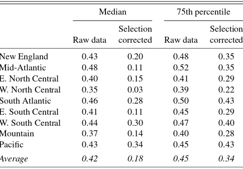
we report those returns in Table8. Returns are analogously
de-fined at the 75th percentile. In every region, the returns to a
col-lege education fall once we control for Roy sorting. Like Dahl (2002), we find significant evidence of an upward bias in the returns to a college education because of Roy sorting, although we generally find that this bias is larger. On average, our mea-sure of returns falls from 42% to 18% at the median and from 45% to 34% at the 75th percentile. Keeping in mind the poten-tial vulnerabilities of our estimator to “home advantage” (i.e., violation of the general commonality assumption) or correlated wage draws (i.e., violation of the independence assumption), these results suggest that observed wage distributions, which are distorted by Roy sorting, seriously overstate the true returns
Table 6. Taste parameter estimates. College graduates
Destination region
New Mid- E. North W. North South E. South W. South
Birth region England Atlantic Central Central Atlantic Central Central Mountain Pacific New England 0 −0.745 −0.578 −1.361 −0.540 −1.068 −0.492 −0.435 −0.448 (0.02) (0.01) (0.03) (0.01) (0.03) (0.01) (0.01) (0.01) Mid-Atlantic −0.614 0 −0.602 −0.351 −0.347 −1.004 −0.700 −0.294 −0.622 (0.01) (0.01) (0.01) (0.01) (0.04) (0.02) (0.01) (0.01) E. North Central −0.562 −1.087 0 −0.798 −0.515 −0.932 −0.647 −0.679 −0.341 (0.02) (0.03) (0.03) (0.01) (0.02) (0.02) (0.02) (0.01) W. North Central −0.475 −0.672 −0.420 0 −0.908 −1.238 −0.861 −0.573 −0.647 (0.01) (0.02) (0.01) (0.02) (0.05) (0.02) (0.01) (0.02) South Atlantic −1.097 −0.975 −0.821 −1.303 0 −0.958 −0.890 −0.858 −0.835 (0.02) (0.03) (0.02) (0.03) (0.02) (0.02) (0.02) (0.02) E. South Central −1.129 −1.063 −0.631 −0.450 −0.513 0 −0.646 −0.924 −0.803 (0.04) (0.03) (0.01) (0.01) (0.01) (0.02) (0.02) (0.02) W. South Central −0.781 −1.330 −0.972 −0.632 −0.630 −0.136 0 −0.823 −0.693 (0.02) (0.04) (0.03) (0.02) (0.01) (0.00) (0.02) (0.02) Mountain −1.106 −1.186 −0.663 −0.840 −0.542 −0.898 −0.666 0 −0.442 (0.03) (0.04) (0.01) (0.02) (0.01) (0.02) (0.02) (0.01) Pacific −1.253 −1.125 −0.861 −0.809 −0.654 −0.499 −0.761 −0.443 0
(0.05) (0.08) (0.02) (0.02) (0.02) (0.01) (0.02) (0.01)
Jour
nal
of
Business
&
Economic
Statistics
,
A
pr
il
2011
Figure 1. High school graduates. Conditional and unconditional log wage distributions by destination region.
y
e
r,
Khan,
and
Timmins:
R
o
y
Model
With
Common
N
onpecuniar
y
R
etur
ns
213
Figure 2. College graduates. Conditional and unconditional log wage distributions by destination region.
Table 7. Log wages by education and region. 2000 U.S. Census, 5% IPUMS random sample. Raw data and corrected for spatial selection
High School College
Median 75th percentile Median 75th percentile Selection Selection Selection Selection Raw data corrected Raw data corrected Raw data corrected Raw data corrected New England 2.77 2.67 3.03 2.97 3.20 2.87 3.51 3.32 Mid-Atlantic 2.76 2.65 3.04 2.97 3.24 2.76 3.56 3.32 E. North Central 2.74 2.61 3.03 2.96 3.14 2.76 3.44 3.25 W. North Central 2.63 2.50 2.92 2.83 2.98 2.53 3.31 3.05 South Atlantic 2.63 2.55 2.93 2.87 3.09 2.83 3.43 3.3 E. South Central 2.60 2.48 2.91 2.82 3.01 2.59 3.36 3.11 W. South Central 2.60 2.48 2.92 2.84 3.04 2.78 3.39 3.24 Mountain 2.67 2.49 2.96 2.86 3.04 2.63 3.36 3.14 Pacific 2.79 2.63 3.07 2.97 3.22 2.97 3.52 3.4
Average 2.69 2.56 2.98 2.90 3.11 2.75 3.43 3.24
to a college education, particularly for those in the heart of the wage distribution.
7. CONCLUSION
This article considers identification and estimation of a multisector Roy model that includes a common nonpecuniary component of utility associated with each alternative. Two iden-tification results are established, one under an extreme quan-tile independence condition and the other under a commonal-ity/independence assumption, where commonality provides us with a convenient exclusion restriction that facilitates identifi-cation. Estimation procedures based on both identification re-sults are proposed, and their asymptotic properties are derived. These models are able to identify the common taste parameter explicitly, and they provide identification in a data environment where the approach used in previous work (i.e., identification at infinity) might prove difficult.
Our second estimator is used to recover an estimate of the re-turns to a college education, controlling for different migration rates of high school and college graduates. We report the values of the taste parameters that, along with wage draws, determine migration decisions, and we recover nonparametric estimates
Table 8. Percentage returns to college education
Median 75th percentile Selection Selection Raw data corrected Raw data corrected New England 0.43 0.20 0.48 0.35 Mid-Atlantic 0.48 0.11 0.52 0.35 E. North Central 0.40 0.15 0.41 0.29 W. North Central 0.35 0.03 0.39 0.22 South Atlantic 0.46 0.28 0.50 0.43 E. South Central 0.41 0.11 0.45 0.29 W. South Central 0.44 0.30 0.47 0.40 Mountain 0.37 0.14 0.40 0.28 Pacific 0.43 0.34 0.45 0.43
Average 0.42 0.18 0.45 0.34
of the unconditional wage distributions from which individu-als receive draws. The results suggest that an estimate based on conditional distributions may overstate returns by more than a factor of 2 at the median. An application of our first estimator to sorting across occupations, where individuals care about pe-cuniary returns and other job attributes (including fatality risk) yields similarly stark results. In that analysis, the wage-hedonic estimate of the value of a statistical life rises by a factor of 4 and becomes statistically significant (Deleire, Khan, and Tim-mins2009).
Finally, it is important to note that the models that we have develop here could be applied to estimate a “generalized” ver-sion of the competing-risks model. Specifically, the “risk” in-dicator is no longer simply determined by the minimum of the two variables whose distributions one aims to identify. Thus it would be useful to further explore how the results attained here can be useful in some of the variations introduced in that litera-ture, allowing for data complications such as left truncation and length-biased sampling.
SUPPLEMENTAL MATERIALS
Appendix: The supplemental materials section contains the
following appendices (outline_appendix.pdf):
- Finite Lower Support Estimator WithKAlternatives
- Kaplan–Meier Procedure
- Derivation of Unbounded Support Estimator
- Asymptotic Properties of Proposed Minimum Distance
Estimator forτ.
ACKNOWLEDGMENTS
We thank Richard Blundell, James Heckman, Hide Ichimura, Robert Moffitt, Tiemen Woutersen, and seminar participants at SUNY Albany, Duke University, Johns Hopkins University, and the University of Chicago for their helpful comments. All re-maining errors and omissions are our own.
[Received April 2008. Revised January 2010.]
REFERENCES
Ahn, H., and Powell, J. L. (1993), “Semiparametric Estimation of Censored Selection Models With a Nonparametric Selection Mechanism,”Journal of Econometrics, 58, 3–29. [202]
Chernozhukov, V., and Hong, H. (2004), “Likelihood Estimation and Infer-ence in a Class of Nonregular Econometric Models,”Econometrica, 72 (5), 1445–1480. [206]
Dahl, G. (2002), “Mobility and the Return to Education: Testing a Roy Model With Multiple Markets,”Econometrica, 70 (6), 2367–2420. [202,209,211] Davies, P. S., Greenwood, M. J., and Li, H. (2001), “A Conditional Logit
Ap-proach to U.S. State-to-State Migration,”Journal of Regional Science, 41 (2), 337–360. [202]
Deleire, T., Khan, S., and Timmins, C. (2009), “Roy Model Sorting and Non-Random Selection in the Valuation of a Statistical Life,” a Nicholas Institute working paper, Duke University. [210,214]
D’Haultfoeuille, X., and Maurel, A. (2010), “Interference on a Generalized Roy Model, With an Application to Schooling Decisions in France,” working paper, CREST. [204]
Falaris, E. (1987), “A Nested Logit Migration Model With Selectivity,” Inter-national Economic Review, 28, 429–443. [202]
Fleming, T. R., and Harrington, D. P. (1991),Counting Processes and Survival Analysis, New York: Wily Brothers. [206]
Hansen, B. (2000), “Sample Splitting and Threshold Estimation,” Economet-rica, 68 (3), 575–603. [204]
Heckman, J. (1990), “Varieties of Selection Bias,”American Economic Review, 80 (2), 313–318. [201]
Heckman, J., and Honore, B. (1989), “The Identifiability of the Competing Risk Model,”Biometrika, 76, 325–330. [201]
(1990), “The Empirical Content of the Roy Model,”Econometrica, 58, 1121–1149. [201,202]
Heckman, J., and Vytlacil, E. (2008), “Econometric Evaluation of Social Pro-grams, Part I,”Handbook of Econometrics, 8, 4779–5144. [203,204] Honore, B. (2002), “Nonlinear Models With Panel Data,”Portuguese Economic
Journal, 1 (2), 163–179. [202]
Honore, B., and Lleras-Muney, A. (2006), “Bounds in Competing Risks Models and the War on Cancer,”Econometrica, 74, 1675–1698. [202]
Kaplan, E. L., and Meier, P. (1958), “Nonparametric Estimation From Incom-plete Data,”Journal of the American Statistical Association, 53, 457–481. [202,204]
Khan, S., and Tamer, E. (2009), “Interference on Endogenously Censored Regression Models Using Conditional Moment Inequalities,” Journal of Econometrics, 52, 104–119. [202]
Lee, L.-F. (1983), “Generalized Econometric Models With Selectivity,” Econo-metrica, 51, 507–512. [202]
Lee, S. (2006), “Identification of Competing Risks Model With Unknown Transformation of Latent Failure Times,”Biometrika, 93, 996–1002. [202] Lee, S., and Lewbel, A. (2009), “Nonparametric Identification of Accelerated Failure Time Competing Risks Models,” working paper, University College London. [202]
Lee, S., and Seo, M. H. (2008), “Semiparametric Estimation of a Binary Re-sponse Model With a Change-Point Due to a Covariate Threshold,”Journal of Econometrics, 144, 492–499. [204]
Newey, W. K., and McFadden, D. (1994), “Estimation and Hypothesis Testing in Large Samples,” inHandbook of Econometrics, Vol. 4, eds., R. F. Engle and D. McFadden, Amsterdam: North-Holland. [207]
Petersen, A. V. (1976), “Bounds for a Joint Distribution With Fixed Sub-Distribution Functions,”Proceedings of the National Academy of Science, 73, 11–13. [202,204]
Porter, J., and Hirano, K. (2003), “Asymptotic Efficiency in Parametric Struc-tural Models With Parameter Dependent Support,”Econometrica, 71 (5), 1307–1338. [206]
Powel, J. L. (1994), “Estimation of Semiparametric Models,” inHandbook of Econometrics, Vol. 4 (1st ed.), eds. R. F. Engle and D. McFadden, Elsevier, pp. 2443–2521. [201]
Roback, J. (1982), “Wages, Rents, and the Quality of Life,”Journal of Political Economy, 90, 1257–1278. [202]
Roy, A. D. (1951), “Some Thoughts on the Distribution of Earnings,”Oxford Economic Papers, 3, 135–146. [201,209]
van der Vaart, A. W. (1998),Asymptotic Statistics, Cambridge, U.K.: Cam-bridge University Presss. [206]