Full Terms & Conditions of access and use can be found at
http://www.tandfonline.com/action/journalInformation?journalCode=ubes20
Download by: [Universitas Maritim Raja Ali Haji] Date: 11 January 2016, At: 22:36
Journal of Business & Economic Statistics
ISSN: 0735-0015 (Print) 1537-2707 (Online) Journal homepage: http://www.tandfonline.com/loi/ubes20
Dynamic Equicorrelation
Robert Engle & Bryan Kelly
To cite this article: Robert Engle & Bryan Kelly (2012) Dynamic Equicorrelation, Journal of Business & Economic Statistics, 30:2, 212-228, DOI: 10.1080/07350015.2011.652048
To link to this article: http://dx.doi.org/10.1080/07350015.2011.652048
View supplementary material
Accepted author version posted online: 12 Jan 2012.
Submit your article to this journal
Article views: 751
View related articles
Supplementary materials for this article are available online. Please go tohttp://tandfonline.com/r/JBES
Dynamic Equicorrelation
Robert E
NGLEStern School of Business, New York University, 44 W. 4th St. Suite 9-190, New York, NY 10012 ([email protected])
Bryan K
ELLYBooth School of Business, University of Chicago, 5807 S. Woodlawn Ave., Chicago, IL 60637 ([email protected])
A new covariance matrix estimator is proposed under the assumption that at every time period all pairwise correlations are equal. This assumption, which is pragmatically applied in various areas of finance, makes it possible to estimate arbitrarily large covariance matrices with ease. The model, called DECO, involves first adjusting for individual volatilities and then estimating correlations. A quasi-maximum likelihood result shows that DECO provides consistent parameter estimates even when the equicorrelation assumption is violated. We demonstrate how to generalize DECO to block equicorrelation structures. DECO estimates for U.S. stock return data show that (block) equicorrelated models can provide a better fit of the data than DCC. Using out-of-sample forecasts, DECO and Block DECO are shown to improve portfolio selection compared to an unrestricted dynamic correlation structure.
KEY WORDS: Conditional covariance; Dynamic conditional correlation; Equicorrelation; Multivariate GARCH.
1. INTRODUCTION
Since the first volatility models were formulated in the early 1980s, there have been efforts to estimate multivariate models. The specifications of these models were developed over the past 25 years with a range of papers surveyed by Bollerslev, Engle, and Nelson (1994) and more recently by Bauwens, Laurent, and Rombouts (2006) and Silvennoinen and Terasvirta (2008). A general conclusion from this analysis is that it is difficult to esti-mate multivariate GARCH models with more than half a dozen return series because the specifications are so complicated.
Recently, Engle (2002) proposed Dynamic Conditional Cor-relation (DCC), greatly simplifying multivariate specifications. DCC is designed for high-dimensional systems but has only been successfully applied to up to 100 assets by Engle and Sheppard (2005). As the size of the system grows, estimation becomes increasingly cumbersome. For cross-sections of hun-dreds or thousands of stocks, as are common in asset pricing applications, estimation can break down completely.
Approaches exist to address the high-dimension problem, though each has limitations. One type of approach is to im-pose structure on the system such as a factor model. Univariate GARCH dynamics in factors can generate time-varying corre-lations while keeping the residual correlation matrix constant through time. This idea motivated the Factor ARCH models of Engle, Ng, and Rothschild (1990,1992) and Engle’s (2009b) Factor Double ARCH. The benefit of these models is their fea-sibility for large numbers of variates: If there arendependent variables andkfactors, estimation requires onlyn+kGARCH models. Furthermore, it uses a full likelihood and will be ef-ficient under appropriate conditions. One drawback is that it is not always clear what the factors are, or factor data may not be available. Another is that correlation dynamics can ex-ist in residuals even after controlling for the factors, as in the case of U.S. equity returns (Engle2009a,b; Engle and Rangel
2012). Addressing either of these problems leads back to the
unrestricted DCC specification, and thus to the dimensionality dilemma.
A second solution uses the method of composite likelihood. This method was recently proposed by Engle, Shephard, and Sheppard (2008) to estimate unrestricted DCC for vast cross-sections. Composite likelihood overcomes the dimension limi-tation by breaking a large system into many smaller subsystems in a way that generalizes the “MacGyver” method of Engle (2009a,b). This approach possesses great flexibility, but will generally be inefficient due to its reliance on a partial likelihood. The contrast of Factor ARCH and composite likelihood high-lights a fundamental tradeoff in large-system conditional covari-ance modeling. Imposing structure on the covaricovari-ance can make estimation feasible and, if correctly specified, efficient; but it sacrifices generality and can suffer from breakdowns due to misspecification. On the other hand, less structured models like composite likelihood break the curse of dimensionality while maintaining a general specification. However, its cost is a loss of efficiency from using a partial likelihood.
We propose a solution to this tradeoff that selectively com-bines simplifying structural assumptions and composite like-lihood versatility. We consider a system in which all pairs of returns have the same correlation on a given day, but this corre-lation varies over time. The model, called Dynamic Equicorre-lation (DECO), eliminates the computational and presentational difficulties of high-dimension systems. Because equicorrelated matrices have simple analytic inverses and determinants, like-lihood calculation is dramatically simplified and optimization becomes feasible for vast numbers of assets.
DECO’s structure can be substantially weakened by us-ing block equicorrelated matrices, while maintainus-ing the
© 2012American Statistical Association Journal of Business & Economic Statistics April 2012, Vol. 30, No. 2 DOI:10.1080/07350015.2011.652048
212
simplicity and robustness of the basic DECO formulation. A block model may capture, for instance, industry correlation structures. All stocks within an industry share the same correla-tion while correlacorrela-tions between industries take another value. In the two-block setting, analytic inverses and determinants are still available and fairly simple, thus optimization for the two-Block DECO model is as easy as the one-block case. The two-block structure can also be combined with the method of composite likelihood to estimate Block DECO with an arbitrary number of blocks. Since the subsets of assets used in Block DECO are pairs of blocks rather than pairs of assets, a larger portion of the likelihood (and therefore more information) is used for op-timization. As a result, the estimator can be more efficient than unrestricted composite likelihood DCC.
Another way to enrich dependence beyond equicorrelation is to combine DECO with Factor (Double) ARCH. To understand how this may work, consider a model in which one factor is observable and the dispersion of loadings on this factor is high. Further, suppose each asset loads roughly the same on a second, latent, factor. The first factor contributes to diversity among pairwise correlations, and is clearly not driven by noise. Thus, DECO may be a poor candidate for describing raw returns. However, residuals from a regression of returns on only the first factorwillbe well described by DECO. One way to model this dataset is to use Factor Double ARCH with DECO residuals. Such a model is estimated by first using GARCH regression models for each stock, then applying DECO to the standardized residuals.
What will occur if DECO is applied to variables that arenot
equicorrelated? If (block) equicorrelation is violated, DECO can still provide consistent parameter estimates. In particular, we prove quasi-maximum likelihood results showing that if DCC is a consistent estimator, then DECO and Block DECO will be consistent also. This means that when the true model is DCC, DECO makes estimation feasible when the dimension of the system may be otherwise too large for DCC to handle. While DECO is closely related to DCC, the two models are nonnested: DECO is not simply a restricted version of DCC, but a competing model. Indeed, DECO possesses some subtle, though important, features lacking in DCC. A key example is that DECO correlations between any pair of assetsiandjdepend on the return histories of all pairs. For the analogous DCC specification (i.e., using the same number of parameters), the i, jcorrelation depends on the histories ofiandjalone. In this sense, DECO parsimoniously draws on a broader information set when formulating the correlation process of each pair. To the extent that true correlations are affected by realizations of all assets, the failure of DCC to capture the information pooling aspect of DECO can disadvantage DCC as a descriptor of the data-generating process.
In a one-factor world, the relation between the return on an asset and the market return is
rj =βjrm+ej, σj2=β 2 jσ
2 m+vj.
If the cross-sectional dispersion ofβjis small and idiosyncrasies
have similar variance over each period, then the system is well-described by Dynamic Equicorrelation. A natural application for this one-factor structure lies in the market for credit derivatives such as collateralized debt obligations, or CDOs. A key feature of the risk in loan portfolios is the degree of correlation
be-tween default probabilities. A simple industry valuation model allows this correlation to be one number if firms are in the same industry and a different and smaller number if they are in differ-ent industries. Hence, within each industry, an equicorrelation assumption is being made.
More broadly, to price CDOs, an assumption is often made that these are large homogeneous portfolios (LHPs) of corporate debt. As a consequence, each asset will have the same variance, the same covariance with the market factor, and the same id-iosyncratic variance. Thus, in an LHP, thejsubscripts disappear. The correlation between any pair of assets then becomes
ρ = β
In fact, the LHP assumption implies equicorrelation.
The equicorrelation assumption also surfaces in derivatives trading. For instance, a popular position is to buy an option on a basket of assets and then sell options on each of the compo-nents, sometimes called a dispersion trade. By delta hedging each option, the value of this position depends solely on the cor-relations. Let the basket have weights given by the vectorw, and let the implied covariance matrix of components of the basket be given by the matrixS. Then, the variance of the basket can be expressed asσ2=w′Sw.In general, we only know about the variances of implied distributions, not the covariances. Hence, it is common to assume that all correlations are equal, giving σ2=n
As a consequence, the value of this position depends upon the evolution of the implied correlation. When each of the variances is a variance swap made up of a portfolio of options, the full position is called a correlation swap. As the implied correlation rises, the value of the basket variance swap rises relative to the component variance swaps.
There is substantial history of the use of equicorrelation in economics. In early studies of asset allocation, Elton and Gru-ber (1973) found that assuming all pairs of assets had the same correlation reduced estimation noise and provided superior port-folio allocations over a wide range of alternative assumptions. Berndt and Savin (1975) studied what could be called equiauto-correlation matrices in production factor and consumer demand systems as a means of working with singular error variance matrices. Ledoit and Wolf (2004) used Bayesian methods for shrinking the sample correlation matrix to an equicorrelated target and showed that this helps select portfolios with low volatility compared to those based on the sample correlation. Further prescriptions for avoiding the notorious noisiness of un-restricted sample correlations and betas abound in the literature (Ledoit and Wolf2003,2004; Michaud1989; Jagannathan and Ma2003; Jobson and Korkie1980; and Meng, Hu, and Bai2011, among others). Ledoit and Wolf’s Bayesian shrinkage and Elton and Gruber’s parameter averaging are different approaches to noise reduction in unconditional correlation estimation. While the Bayesian method has not yet been employed for conditional variances, DECO makes it possible to incorporate Elton and Gruber’s noise reduction technique into a dynamic setting. By
averaging pairwise correlations, (Block) DECO smooths cor-relation estimates within groups. As long as this reduces es-timation noise more than it compromises the true correlation structure, smoothing can be beneficial. Our empirical results suggest that the benefits of smoothing indeed extend to the con-ditional case. Across a range of first-stage factor models, (Block) DECO selects out-of-sample portfolios that have significantly lower volatilities than those chosen by unrestricted DCC.
The next section develops the DECO model and its theo-retical properties. Section 3 presents Monte Carlo experiments that assess the model’s performance under equicorrelated and nonequicorrelated generating processes. In Section 4, we ap-ply DECO, Block DECO, and DCC models to U.S. stock return data. We find that DCC correlations between pairs of stocks have a large degree of comovement, suggesting that DECO may be beneficial in describing the system’s correlation. Indeed, we find that basic DECO, and DECO with 10 industry blocks, provide a better fit of the data than DCC. Finally, we analyze the abil-ity of (Block) DECO to construct optimal out-of-sample hedge portfolios. We find that (Block) DECO is the model that most often delivers MV portfolios with the lowest sample variance.
2. THE DYNAMIC EQUICORRELATION MODEL
We begin by defining an equicorrelation matrix and present a result for its invertibility and positive definiteness that will be useful throughout the article.
Definition 2.1 A matrix Rt is anequicorrelation matrixof
ann×1 vector of random variables if it is positive definite and takes the form
Rt =(1−ρt)In+ρtJn, (2)
where ρt is the equicorrelation, Indenotes then-dimensional
identity matrix, and Jnis then×nmatrix of ones.
Lemma 2.1 The inverse and determinant of the equicorrela-tion matrix,Rt, are given by
Proofs are provided in the online appendix.
Definition 2.2 A time series of n×1 vectors {r˜t} obeys
a Dynamic Equicorrelation (DECO) model if vart−1(˜rt)= DtRtDt, where Rt is given by Equation (2) for all tand Dt
is the diagonal matrix of conditional standard deviations of ˜rt.
The dynamic equicorrelation isρt.
2.1 Estimation
Like many covariance models, a two-stage quasi-maximum likelihood (QML) estimator of DECO will be consistent and asymptotically normal under broad conditions including many forms of model misspecification. We provide asymptotic results
here for a general framework that includes several standard mul-tivariate GARCH models as special cases, including DECO and the original DCC model. The development is a slightly mod-ified reproduction of the two-step QML asymptotics of White (1994). After presenting the general result, we elaborate on prac-tical estimation of DECO using Gaussian returns and GARCH covariance evolution.
First, define the (scaled) log quasi-likelihood of the model as L({r˜t},θ,φ)=T1 Tt=1logft(˜rt,θ,φ), which is parameterized
by vectorγ =(θ,φ)∈Ŵ=×. The two-step estimation problem may be written as
max
where ˆθis the solution to (5). The full two-stage QML estimator for this problem is ˆγ = ( ˆθ, ˆφ), where ˆφ is the second-stage maximizer solving (6) given ˆθ. Under the technical assumptions listed in the online appendix, White (1994) proves the following result for consistency and asymptotic normality of ˆγ.
Conjecture 2.1 (White1994, theorem 6.11)Under Assump-tions B.1 through B.6 in the online appendix,
√
In the remainder of the section, we assume that both DECO and DCC log densities and their derivatives satisfy Assumptions B.1–B.4 and B.6 of Conjecture 2.1. These are high-level as-sumptions about continuity, differentiability, boundedness, and the applicability of central limit theorems. Further, we assume that the DCC model is identified, and this takes the form of Assumption B.5. Note that we have not verified these assump-tions for the generating processes that we consider in this article. The dynamic covariance literature uniformly appeals to QML asymptotic theory when performing inference, though satisfac-tion of high-level assumpsatisfac-tions has not been established forany
model that has been proposed in this area. A rigorous analysis of asymptotic theory for multivariate GARCH processes remains an important unanswered question. For this reason, we refer to any result that follows immediately from White’s (1994) Theo-rem 6.11 as a conjecture. We refer readers to the online appendix for more detail on this point, as well as simulation evidence that supports the satisfaction of these high-level assumptions for the DECO model.
DECO is adopted for individual applications by specifying a conditional volatility model (i.e., defining the process for Dt)
and aρtprocess. We assume that each conditional volatility
fol-lows a GARCH model. We work with volatility-standardized
returns, denoted by omitting the tilde, rt = D−t1˜rt, so that
vart−1(rt)=Rt.
The basicρtspecification we consider derives from the DCC
model of Engle (2002) and its cDCC modification proposed by Aielli (2009). The correlation matrix of standardized returns,
RDCCt , is given by
where ˜Qt replaces the off-diagonal elements of Qt with
ze-ros but retains its main diagonal and ¯Q is the unconditional covariance matrix of standardized residuals.
DECO setsρtequal to the average pairwise DCC correlation
RDECOt =(1−ρt)In+ρtJn×n, (9)
whereqi,j,t is thei, jth element of Qt. The following
assump-tion and lemma ensure that DECO possesses certain properties important for dynamic correlation models.
Assumption 2.1 The matrix ¯Qis positive definite,α+β <1, α >0, andβ >0.
Lemma 2.2 Under Assumption 2.1, the correlation matrices generated by every realization of a DECO process according to Equations (7) through (10) are positive definite and the process is mean reverting.
The result states that, for any correlation matrix, the trans-formation to equicorrelation shown in Equations (9) and (10) results in a positive-definite matrix. The bounds (n−−11,1) forρt
are not assumptions of the model, but are guaranteed by this transformation as long asRDCC
t is positive definite. As will be
seen in our later discussion of Block DECO, bounds on permis-sible correlation values become looser as the number of blocks increases.
We estimate DECO with Gaussian quasi-maximum likeli-hood, which embeds it in the framework of Conjecture 2.1. Con-ditional on past realizations, the return distribution is ˜rt|t−1∼
N(0,Ht),Ht =DtRtDt.To establish notation, we use
super-scripted densitiesftDECOandftDCCto indicate the Gaussian den-sity of ˜rt|t−1assuming the covariance specifically obeys DECO
or DCC, respectively. Similarly, superscripted log-likelihoods LDECOandLDCCrepresent the log-likelihood of DECO or DCC. Omission of superscripts will be used to discuss densities and log-likelihoods without specific assumptions on the dynamics or structure of covariance matrices.
The multivariate Gaussian log-likelihood functionL can be decomposed (suppressing constants) as
Letθ ∈andφ∈denote the vector of univariate volatility parameters and the vector of correlation parameters, respec-tively. The above equation says that the log-likelihood can be separated additively into two terms. The first term, which we callL(θ), depends on the parameters of the univariate GARCH processes which affect only the Dt matrices and are
indepen-dent of Rt andφ. The second term, which we callLCorr(θ,φ),
depends on both the univariate GARCH parameters (embedded in the rt terms) as well as the correlation parameters. Engle
(2002) and Engle and Sheppard (2005) noted that correlation models of this form satisfy the assumptions of Conjecture 2.1. In particular,LVol(θ) corresponds toL1in the conjecture and ˆθ
is the vector of first-stage volatility parameter estimates.L( ˆθ,φ) corresponds to the second-step likelihood,L2, so ˆφis the
maxi-mizer ofLCorr( ˆθ,φ). Note that the model ensures stationarity and
that the covariance matrix remains positive definite in all peri-ods whenever Assumption 2.1 holds and the univariate GARCH models are stationary.
The vector ˆγDECOis the two-stage Gaussian estimator when the second-stage likelihood obeys DECO. It assumes returns are Gaussian and the correlation process obeys Equations (9) and (10). The following conjectures specifically apply Conjecture 2.1 to the Gaussian DECO and DCC models.
Conjecture 2.2 Assuming thatfDECO
t andLDECOsatisfy
As-sumptions B.1–B.6 with corresponding unique maximizerγ∗, then ˆγDECOis consistent and asymptotically normal forγ∗.
The analogous corollary for ˆγDCC, the two-stage Gaussian DCC estimator, will be useful in developing our later compari-son between DECO and DCC.
Conjecture 2.3 Assuming thatftDCCand LDCC satisfy As-sumptions B.1–B.6 with corresponding unique maximizerγ∗, then ˆγDCCis consistent and asymptotically normal forγ∗.
In addition, the asymptotic covariance matrices for ˆγDECO
and ˆγDCC corresponding to Conjectures 2.2 and 2.3 take the form stated in Conjecture 2.1, replacing L1 andL2 with the
appropriately superscripted likelihoodsL(Vol·) andL(Corr·) .
To appreciate the payoff from making the equicorrelation assumption, consider the second step likelihood under DECO
LDECOCorr ( ˆθ,φ)
where ˆrt are returns standardized for first-stage volatility
esti-mates, ˆrt =Dt( ˆθ)−1˜rt, andρt obeys Equation (10). In DCC,
the conditional correlation matrices must be recorded and in-verted for alltand their determinants calculated; further, these
Tinversions and determinant calculations are repeated for each of the many iterations required in a numeric optimization pro-gram. This is costly for small cross-sections and potentially infeasible for very large ones. In contrast, DECO reduces com-putation ton-dimensional vector outer products with no matrix inversions or determinants required, rendering the likelihood optimization problem manageable even for vast-dimensional systems. The likelihood at timet can be calculated from just three statistics, the average cross-sectional standardized return, the average cross-sectional squared standardized return, and the predicted correlation. This is a simple calculation in all settings considered in this article.
2.2 Differences Between DECO and DCC
The transformation from DCC correlations to DECO in Equa-tion (10) introduces subtle differences between the DECO and DCC likelihoods. The two models are nonnested; they share the same number of parameters and there is no parameter restric-tion that makes the models identical. The correlarestric-tion matrix for DCC is nonequicorrelated in all realizations, while, by defini-tion, DECO is always exactly equicorrelated.
Both models build off of the Q process in (7). On a given day, Q is updated as a function of the lagged return vector and the lagged Q matrix. From here, Q is transformed to
RDCC = Q˜−
1 2 t QtQ˜−
1 2
t .RDCCis the correlation matrix that enters
the DCC likelihood. Note that thei, jelement of this matrix is qi,j,t/√qi,i,tqj,j,t. Clearly, the information about pairi, j’s
cor-relation at timetdepends on the history of assetsiandjalone. On the other hand, the correlation betweeniandjunder DECO is ρt = n(n2−1)i>j
qi,j,t
√q
i,i,tqj,j,t,which depends on the history ofall
pairs. The failure of DCC to capture this information-pooling aspect of DECO correlations hinders the ability of the DCC likelihood to provide a good description of the data-generating process, resulting in poor estimation performance, as will be seen in the Monte Carlo results of Section 3.
There is also a key difference that arises from the need to es-timate DCC with a partial, composite likelihood. When DECO is the true model, DCC estimation is akin to estimating the correlation of a single pair, sampledn(n−1)/2 times. The dif-ference between each pair is the measurement error. DECO, by averaging pairwise correlations at each step, attenuates this measurement error. It also uses the full cross-sectional likeli-hood rather than a partial one like composite likelilikeli-hood.
2.3 DECO as a Feasible DCC Estimator
Often the equicorrelation assumption fails so that there is cross-sectional variation in pairwise correlations, as in DCC. In this case, the DECO model remains a powerful tool. The following result shows that as long as DCC is a Gaussian QML estimator, DECO will be also.
Proposition 2.1 Assume thatftDECO andLDECO satisfy As-sumptions B.1–B.4 and B.6, and assume that the DCC model is identified and therefore satisfies Assumption B.5. Then, As-sumption B.5 is guaranteed to be satisfied for the DECO model, so that ˆγDECOis identified and hence DECO is a consistent and asymptotically normal estimator forγ∗.
Suppose that DCC is the true model and that the high-level regularity conditions on the densities of DCC and DECO (differ-entiability and boundedness, etc.) are satisfied, but that DECO is notassumedto be identified. Then, Proposition 2.1guarantees
that DECO is identified, therefore it consistently estimates the true DCC parameters. Furthermore, the asymptotic covariance matrix for ˆγDECO takes the form stated in Conjecture 2.1 (re-placingL1 andL2 withLDECOVol andL
DECO
Corr ) since Proposition
2.1 in turn satisfies the conditions of Conjecture 2.2.
2.4 Estimation Structure Versus Fit Structure
How useful is Proposition 2.1 in practice? Suppose, for in-stance, the system is so large that DCC estimation based on full maximum likelihood is infeasible. The result says that one can consistently estimate DCC parameters using DECO de-spite its misspecification. The estimated parameters can then be plugged into Equation (7) to reconstruct the unrestricted DCC-fitted process. In short, DECO, like composite likelihood, pro-vides feasible estimates for a DCC model that may be otherwise computationally infeasible.
The flexibility of DECO goes beyond its ability to fit unre-stricted DCC processes. The logic of Proposition 2.1 ensures that DECO can consistently estimate block equicorrelation pro-cesses as well. To do this,αandβ are estimated with DECO, then data are run through the evolution equation in (7), plug-ging in ˆαDECOand ˆβDECO. The resulting DCC correlation series,
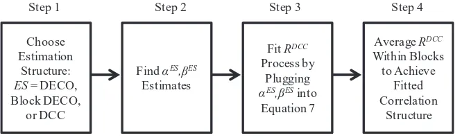
based on DECO estimates, can be used to construct any fitted block correlation structure by averaging pairwise DCC correla-tions within blocks (see schematic inFigure 1).
Throughout the remaining sections, we will refer to “estima-tion structures” and “fit structures,” and it is important to draw
Choose Estimation
Structure:
ES= DECO, Block DECO,
or DCC
Find ES, ES Estimates
Fit RDCC Process by
Plugging ES, ESinto
Equation 7
Average RDCC Within Blocks
to Achieve Fitted Correlation
Structure
Step 1 Step 2 Step 3 Step 4
Figure 1. Procedure for generating fitted correlation structures. The schematic diagram summarizes how a correlation structure used as part of the maximum likelihood estimation procedure, what we call the “estimation structure,” can differ from the “fit structure” of the correlation series eventually generated from the estimated model.
the distinction between them. The estimation structure is the structure that the correlation matrix takeswithin the likelihood. When DECO is used, the estimation structure is a single block. The fit structure, on the other hand, refers to the structure of the final, fitted correlation matrices. It is achieved by averaging DCC correlations within blocksafterestimation. The resulting block structure can be different from the estimation structure and might have one block, many blocks, or be unrestricted (as in DCC).
In the next section, we present an alternative estimation ap-proach called Block DECO. Block DECO directly models the block correlation structure ex ante and makes use of it within the estimation procedure. In this case, the estimation structure will be allowed to have multiple blocks. As with DECO, ex post block averaging can be used to generate a different desired cor-relation fit structure. With Block DECO as the estimator, fitted correlations can have the same, more, or fewer blocks than the estimation structure.
Using DECO with ex post averaging to achieve block cor-relations is, from an implementation standpoint, simpler than using full-fledged Block DECO estimation. As will be shown, Block DECO estimation involves composite likelihood and thus is operationally more complex. Ex post averaging achieves the same outcome of dynamic block correlations with the simplicity of DECO’s Gaussian QML estimation. The advantage of more complicated Block DECO estimation is that it can potentially be more efficient. We turn to that model now.
2.5 The Block Dynamic Equicorrelation Model
While DECO will be consistent even when equicorrelation is violated, it is possible that a loosening of the structure to block equicorrelation can improve maximum likelihood esti-mates. In this vein, we extend DECO to take the block structure into account ex ante and thus incorporate it into the estimation procedure.
As an example of Block DECO’s usefulness, consider model-ing correlation of stock returns with particular interest in intra-and interindustry correlation dynamics. This may be done by imposing equicorrelation within and between industries. Each industry has a single dynamic equicorrelation parameter and each industry pair has a dynamic cross-equicorrelation parame-ter. With block equicorrelation, richer cross-sectional variation is accommodated while still greatly reducing the effective di-mensionality of the correlation matrix.
This section presents the class of block Dynamic Equicorre-lation models and examines their properties.
Definition 2.3 Rtis aK-block equicorrelation matrixif it is
positive definite and takes the form
Rt =
Block DECO specifies that, conditional on the past, each vari-able is Gaussian with mean zero, variance one, and correlations taking the structure in Equation (11). The return vector rt is
partitioned intoKsubvectors; each subvectorrlcontainsnl
re-turns. The Block DECO correlation matrix,RBDt , allows distinct processes for each of theK diagonal blocks andK(K−1)/2 unique off-diagonal blocks. Blocks on the main diagonal have equicorrelations followingρl,l,twhile blocks off the main
diag-onal followρl,m,t, where
ρl,l,t=
correlations are calculated as the average DCC correlation within each block. Despite the block structure of equicorrela-tions, Equation (7) remains the underlying DCC model, thus the parametersαandβ do not vary across blocks. Densities, log-likelihoods, and parameter estimates corresponding to Block DECO model are superscripted with BD in congruence with notation for the base DECO model.
The following results show the consistency and asymptotic normality of Block DECO. In analogy to DECO, ˆγBD is the two-stage Gaussian Block DECO estimator assuming returns are Gaussian and the correlation process obeys Equation (12).
Conjecture 2.4 Assuming thatfBD
t andLBDsatisfy
Assump-tions B.1–B.6 with corresponding unique maximizerγ∗, then ˆ
γBDis consistent and asymptotically normal forγ∗.
Further, like DECO, Block DECO is a QML estimator of DCC models.
Proposition 2.2 Assume thatftBDandLBDsatisfy Assump-tions B.1–B.4 and B.6, and assume that the DCC model is iden-tified and therefore satisfies Assumption B.5. Then, Assumption B.5 is guaranteed to be satisfied for the Block DECO model, so that ˆγBDis identified and hence Block DECO is a consistent and asymptotically normal estimator forγ∗.
The proof follows the same argument as the proof of Propo-sition 2.1. The asymptotic covariance matrix for ˆγBDtakes the form stated in Conjecture 2.1 (replacing L1 andL2 withLBDVol
andLBD Corr).
Block DECO balances the flexibility of unrestricted correla-tions with the structural simplicity of DECO. However, when the number of blocks is greater than two, the analytic forms for the inverse and determinant of the Block DECO matrix begin to lose their tractability. A special case that remains simple regard-less of the number of blocks occurs when each of the blocks on the main diagonal are equicorrelated, but all off-diagonal
block equicorrelations are forced to zero. Each diagonal block constitutes a small DECO submodel, and therefore its inverse and determinant are known. The full inverse matrix is the block diagonal matrix of inverses for the DECO submodels, and its determinant is the product of the submodel determinants.
Conveniently, the composite likelihood method can be used to estimate Block DECO in more general cases. The composite likelihood is constructed by treating each pair of blocks as a submodel, then calculating the quasi-likelihoods of each sub-model, and finally summing quasi-likelihoods over all block pairs. As discussed by Engle et al. (2008), each pair provides a valid, though only partially informative, quasi-likelihood. A model for any number of blocks requires only the analytic in-verse and determinant for a two-block equicorrelation matrix when using the method of composite likelihood. The following lemma establishes the analytic tractability provided by two-block equicorrelation. We suppresstsubscripts as all terms are contemporaneous.
Lemma 2.3 If Ris a two-block equicorrelation matrix, that is, if
i. the inverse is given by
R−1=
ii. the determinant is given by
det(R)=(1−ρ1,1)n1−1(1−ρ2,2)n2−1
×(1+[n1−1]ρ1,1)(1+[n2−1]ρ2,2)−ρ12,2n1n2
,
iii. Ris positive definite if and only if
ρi ∈
With this result in hand, the likelihood function of a two-Block DECO model can, as in the simple equicorrelation case, be written to avoid costly inverse and determinant calculations.
L= −1
In the multiblock case, the above two-block log likelihood is calculated for each pair of blocks, and then these submodel likelihoods are summed, forming the objective function to be maximized.
3. CORRELATION MONTE CARLOS
3.1 Equicorrelated Processes
This section presents results from a series of Monte Carlo ex-periments that allow us to evaluate the performance of the DECO framework when the true data-generating process is known. We begin by exploring the model’s estimation ability when DECO is the generating process. Asset return data for 10, 30, or 100 assets are simulated over 1000 or 5000 periods according to Equations (7)–(10). We also consider a range of values forα andβ. For each simulated dataset, we estimate DECO and com-posite likelihood DCC. Here and throughout, we use a subset of n randomly chosen pairs of assets to form the composite likelihood in order to speed up computation. In unreported re-sults, we run a subset of our simulations estimating composite likelihood with alln(n−1)/2 pairs, and results were virtually indistinguishable. Engle et al. (2008) found that the loss from using a subset ofnpairs is negligible.
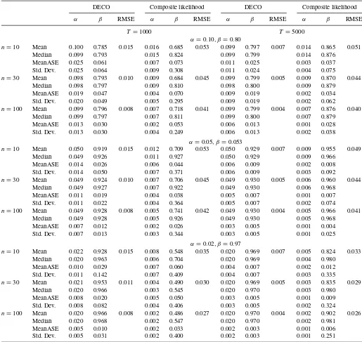
Simulations are repeated 2500 times and summary statis-tics for the maximum likelihood parameter estimates are calcu-lated.Table 1reports the mean, median, and standard deviation ofαandβ estimates, their average QML asymptotic standard
Table 1. Monte Carlo with equicorrelated generating process
DECO Composite likelihood DECO Composite likelihood
α β RMSE α β RMSE α β RMSE α β RMSE
T =1000 T =5000
α=0.10, β=0.80
n=10 Mean 0.100 0.785 0.015 0.016 0.685 0.053 0.099 0.797 0.007 0.014 0.865 0.051 Median 0.099 0.793 0.015 0.824 0.099 0.799 0.014 0.876
MeanASE 0.025 0.061 0.007 0.073 0.011 0.025 0.003 0.037 Std. Dev. 0.025 0.064 0.009 0.308 0.011 0.024 0.004 0.075
n=30 Mean 0.098 0.793 0.010 0.009 0.684 0.045 0.099 0.799 0.005 0.009 0.870 0.044 Median 0.098 0.797 0.009 0.810 0.098 0.800 0.009 0.879
MeanASE 0.019 0.047 0.004 0.070 0.009 0.019 0.002 0.034 Std. Dev. 0.020 0.049 0.005 0.295 0.009 0.019 0.002 0.062
n=100 Mean 0.099 0.796 0.008 0.007 0.718 0.041 0.099 0.799 0.004 0.007 0.876 0.040 Median 0.099 0.797 0.007 0.811 0.099 0.800 0.007 0.879
MeanASE 0.013 0.030 0.002 0.053 0.006 0.013 0.001 0.028 Std. Dev. 0.013 0.030 0.004 0.249 0.006 0.013 0.002 0.038
α=0.05, β=0.053
n=10 Mean 0.050 0.919 0.015 0.012 0.709 0.053 0.050 0.929 0.007 0.009 0.955 0.049 Median 0.049 0.926 0.011 0.927 0.050 0.929 0.009 0.966
MeanASE 0.014 0.026 0.006 0.044 0.006 0.009 0.002 0.008 Std. Dev. 0.014 0.050 0.007 0.371 0.006 0.009 0.003 0.092
n=30 Mean 0.049 0.924 0.010 0.007 0.706 0.045 0.049 0.930 0.005 0.006 0.960 0.044 Median 0.049 0.927 0.007 0.922 0.049 0.930 0.006 0.968
MeanASE 0.011 0.019 0.004 0.038 0.005 0.007 0.001 0.007 Std. Dev. 0.011 0.022 0.004 0.364 0.005 0.007 0.002 0.074
n=100 Mean 0.049 0.928 0.008 0.005 0.741 0.042 0.049 0.930 0.004 0.005 0.966 0.041 Median 0.049 0.928 0.005 0.926 0.049 0.930 0.005 0.968
MeanASE 0.007 0.012 0.002 0.026 0.003 0.005 0.001 0.004 Std. Dev. 0.007 0.013 0.003 0.344 0.003 0.005 0.001 0.025
α=0.02, β=0.97
n=10 Mean 0.022 0.928 0.015 0.008 0.548 0.035 0.020 0.969 0.007 0.005 0.824 0.033 Median 0.020 0.963 0.006 0.704 0.020 0.969 0.004 0.980
MeanASE 0.010 0.029 0.007 0.060 0.004 0.007 0.002 0.012 Std. Dev. 0.011 0.142 0.007 0.409 0.004 0.007 0.003 0.335
n=30 Mean 0.021 0.953 0.011 0.004 0.490 0.030 0.020 0.969 0.005 0.003 0.835 0.029 Median 0.020 0.966 0.003 0.545 0.020 0.970 0.003 0.980
MeanASE 0.008 0.020 0.005 0.050 0.003 0.005 0.001 0.009 Std. Dev. 0.008 0.082 0.004 0.406 0.003 0.005 0.002 0.324
n=100 Mean 0.020 0.966 0.008 0.002 0.486 0.027 0.020 0.970 0.004 0.002 0.902 0.026 Median 0.020 0.968 0.002 0.547 0.020 0.970 0.002 0.981
MeanASE 0.005 0.010 0.002 0.033 0.002 0.003 0.001 0.006 Std. Dev. 0.005 0.031 0.002 0.400 0.002 0.003 0.001 0.251
Using the DECO model of Equations (7)–(10), return data for 10, 30, or 100 assets are simulated over 1000 or 5000 periods using a range of values forαandβ. Then, DECO is estimated with maximum likelihood and DCC is estimated using the (pairwise) composite likelihood of Engle et al. (2008). Simulations are repeated 2500 times and summary statistics are calculated. The table reports the mean, median, and standard deviation ofαandβestimates, as well as their mean quasi-maximum likelihood asymptotic standard error estimates. Asymptotic standard errors are calculated using the “sandwich” covariance estimator of Bollerslev and Wooldridge (1992). We also calculate the root-mean-squared error (RMSE) for the true versus fitted average pairwise correlation process and report the average RMSE over all simulations. Correlation targeting is used in all cases, thus the intercept is the same for both models and not reported.
errors (calculated using the “sandwich” covariance estimator of Bollerslev and Wooldridge1992), and the root-mean-squared error (RMSE) for the true versus fitted average pairwise corre-lation process. Both models use correcorre-lation targeting, thus the intercept matrix is the same for both models and not reported.
The results show that across parameter values, cross-section sizes, and sample lengths, DECO outperforms unrestricted DCC in terms of both accuracy and efficiency. Depending on sim-ulation parameters, DECO is between two to 10 times more accurate than DCC at matching the simulated average
correla-tion path, as measured by RMSE. In small samples, DCC can fare particularly poorly. For example, whenT =1000,n=10 andβ =0.97, DCC’s meanβ estimate is 0.55, versus 0.93 for DECO. Also, DCC’s QML standard errors can grossly under-estimate the true variability of its under-estimates for all sample sizes. The simulations also show that when the data-generating pro-cess is equicorrelation, increasing the number of assets in the cross section improves estimates.
What explains the poor performance of DCC? Some char-acteristics of the DECO likelihood are lacking in DCC, as
discussed in Section 2.2. DCC updates pairwise correlations using pairwise data histories, rather than using the data history of all series as in DECO. Also, the partial information nature of composite likelihood DCC makes it even more difficult for DCC to estimate the parameters of a DECO process.
3.2 Nonequicorrelated Processes
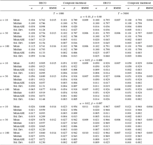
Proposition 2.1 highlights DECO’s ability to consistently es-timate DCC parameters despite violation of equicorrelation. To demonstrate the performance of DECO in this light, we simu-late series using DCC as the data-generating process (Equations (7) and (8)). Thus, while equicorrelation is violated, the aver-age pairwise correlation behaves according to DECO and the assumptions of Conjecture 2.1 are satisfied. In the correlation evolution, we use an intercept matrix that is nonequicorrelated; the standard deviation of off-diagonal elements is 0.33, demon-strating that the differences in pairwise correlations for the sim-ulated cross sections are substantial.
Again, we generate return data for 10, 30, or 100 assets over 1000 or 5000 periods using a range of values forαandβ. Next, we estimate both DECO and composite likelihood DCC.Table 2
reports summary statistics. DECO exhibits a downward bias in itsβ estimates that is exacerbated at low values ofT /N. For largeT /N, theβbias nearly disappears. Composite likelihood performs comparatively well, though the difference in accuracy versus DECO is almost indistinguishable whenT is 5000. The superior performance of DCC is perhaps most clearly seen in its excellent precision. In all cases, the variability of DCC estimates are a fraction of DECO’s.
It appears that DECO’s performance under misspecifica-tion (Table 2) is overall better than DCC’s performance un-der misspecification (Table 1). Small samples generally result in a downward bias in DECO estimates, but these estimates always manage to stay within one standard error of the es-timates achieved by the correctly specified model. This is in contrast to the severe downward biases displayed by DCC in
Table 1. Similarly, DECO’s QML standard errors, while under-stated by an order of magnitude of roughly two, are only mildly biased compared to the performance of DCC’s standard errors in
Table 1.
4. EMPIRICAL ANALYSIS
4.1 Data
Since DECO is motivated primarily as a means of estimating dynamic covariances for large systems, our sample includes constituents of the S&P 500 Index. A stock is included if it was traded over the full horizon 1995–2008 and was a member of the index at some point during that time. This amounts to 466 stocks. Data on returns and SIC codes (which will be used for block assignments) come from the CRSP daily file. In our Factor ARCH regressions and Block DECO estimation, we use Fama–French three-factor return data and industry assignments (based on SICs) from Ken French’s website. Precise definitions of portfolios can be found there.
We also compare average correlations for (Block) DECO and DCC to option implied correlations. For this analysis, we use a
36-stock subset of the S&P sample that were continuously traded over 1995–2008 and were members of the Dow Jones Industrials at some point in that period. We also use daily option-implied volatilities on these constituents and the index from October 1997 through September 2008 from the standardized options file of OptionMetrics.
Before proceeding to the results, we include a brief aside re-garding estimation that will be important for the information criterion comparisons we make throughout. All second-stage correlation models that we estimate have the same number of parameters: anαestimate, aβestimate, andn(n−1)/2 unique elements of the intercept matrix. Each factor structure, however, has a different number of parameters. Residual GARCH models contain a total of 5nparameters. In addition, the loadings in a
K-factor model (including a constant as one of theK factors) contribute an additionalnK parameters. Also, the likelihoods from different composite likelihood methods are not directly comparable because they use submodels of differing dimen-sions. Therefore, we use composite likelihood fitted parameters to evaluate the full joint Gaussian likelihood after the fact, which is directly comparable to the DECO likelihood.
4.2 Dynamic Equicorrelation in the S&P 500, 1995–2008
Our appraisal of DECO has thus far relied on simulated data, now we assess DECO estimates for the S&P 500 sample. As dis-cussed in the section on model estimation, we use a consistent two-step procedure to estimate correlations. In the first stage, we regress individual stock returns on a constant and specify resid-uals to be asymmetric GARCH(1,1) processes with Student-t
innovations (Glosten, Jagannathan, and Runkle1993). GARCH regressions are estimated stock-by-stock via maximum likeli-hood, and then volatility-standardized residuals are given as inputs to the second-stage DECO model. Here and throughout, second-stage models are estimated using correlation targeting for the intercept matrix ¯Q. The first column of Panel A in Ta-ble 3ashows estimates for the basic DECO specification, their standard errors, and the Akaike information criterion (AIC) for the full two-stage log-likelihood.
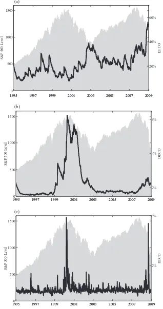
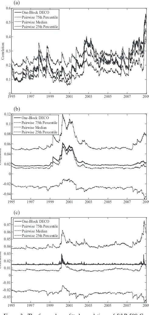
We find ˆα=0.021 and ˆβ =0.979, thus the DECO parame-ters are in the range of typical estimates from GARCH models. Rounded to three decimals places, ˆαand ˆβ sum to one, indi-cating that the equicorrelation is nearly integrated.Figure 2(a) plots the fitted S&P DECO series against the price level of the S&P 500 Index. The clearest feature of the plot is the tendency for the average correlation to rise when the market is decreasing and fall when the market is increasing. This inverse relationship between market value and correlations has been documented previously in the literature. Longin and Solnik (1995,2001) found that correlations between country level indices are higher during bear markets and in volatile periods. Ang and Chen (2002) found the same result for correlations between portfo-lios of U.S. stocks and the aggregate market. Our results show that, over the past 15 years, correlations reached their highest level during the global crisis in the last four months of 2008, when the average correlation between S&P 500 stocks reached nearly 60%.
Table 2. Monte Carlo with nonequicorrelated generating process
DECO Composite likelihood DECO Composite likelihood
α β RMSE α β RMSE α β RMSE α β RMSE
T =1000 T =5000
α=0.10, β=0.80
n=10 Mean 0.104 0.762 0.015 0.101 0.789 0.009 0.100 0.795 0.007 0.100 0.798 0.004 Median 0.100 0.786 0.100 0.791 0.100 0.797 0.100 0.798
MeanASE 0.038 0.098 0.008 0.020 0.016 0.036 0.004 0.008 Std. Dev. 0.038 0.128 0.012 0.027 0.016 0.036 0.005 0.011
n=30 Mean 0.108 0.754 0.013 0.102 0.787 0.006 0.101 0.795 0.006 0.101 0.797 0.003 Median 0.101 0.790 0.102 0.788 0.100 0.797 0.101 0.798
MeanASE 0.047 0.123 0.005 0.011 0.020 0.045 0.002 0.005 Std. Dev. 0.049 0.154 0.007 0.016 0.019 0.045 0.003 0.007
n=100 Mean 0.115 0.741 0.016 0.102 0.788 0.006 0.102 0.791 0.008 0.101 0.798 0.003 Median 0.104 0.793 0.102 0.789 0.100 0.798 0.101 0.798
MeanASE 0.056 0.133 0.002 0.006 0.025 0.057 0.001 0.003 Std. Dev. 0.059 0.184 0.006 0.013 0.025 0.060 0.003 0.006
α=0.05, β=0.009
n=10 Mean 0.052 0.905 0.015 0.051 0.922 0.009 0.050 0.928 0.007 0.050 0.929 0.004 Median 0.050 0.923 0.051 0.922 0.050 0.929 0.050 0.929
MeanASE 0.021 0.042 0.005 0.008 0.009 0.014 0.002 0.003 Std. Dev. 0.022 0.095 0.006 0.010 0.008 0.014 0.003 0.004
n=30 Mean 0.056 0.889 0.013 0.054 0.918 0.007 0.050 0.927 0.006 0.051 0.928 0.003 Median 0.051 0.921 0.054 0.918 0.050 0.929 0.051 0.928
MeanASE 0.028 0.057 0.003 0.004 0.011 0.017 0.001 0.002 Std. Dev. 0.030 0.131 0.004 0.007 0.011 0.019 0.002 0.003
n=100 Mean 0.065 0.877 0.016 0.054 0.918 0.007 0.052 0.926 0.008 0.051 0.928 0.003 Median 0.055 0.919 0.054 0.918 0.051 0.929 0.051 0.928
MeanASE 0.036 0.073 0.001 0.002 0.014 0.022 0.001 0.001 Std. Dev. 0.041 0.148 0.003 0.005 0.014 0.026 0.001 0.002
α=0.02, β=0.097
n=10 Mean 0.026 0.888 0.014 0.023 0.954 0.011 0.020 0.967 0.007 0.021 0.968 0.004 Median 0.021 0.959 0.022 0.956 0.020 0.968 0.021 0.968
MeanASE 0.017 0.093 0.003 0.009 0.005 0.011 0.001 0.002 Std. Dev. 0.019 0.209 0.004 0.013 0.005 0.014 0.002 0.003
n=30 Mean 0.029 0.878 0.012 0.027 0.942 0.009 0.021 0.966 0.006 0.022 0.965 0.003 Median 0.023 0.957 0.027 0.943 0.020 0.969 0.022 0.965
MeanASE 0.020 0.065 0.002 0.006 0.007 0.013 0.001 0.001 Std. Dev. 0.025 0.220 0.003 0.010 0.007 0.015 0.001 0.002
n=100 Mean 0.037 0.860 0.014 0.027 0.942 0.010 0.022 0.964 0.007 0.022 0.965 0.003 Median 0.027 0.951 0.027 0.943 0.021 0.969 0.022 0.965
MeanASE 0.027 0.072 0.001 0.003 0.009 0.017 0.000 0.001 Std. Dev. 0.035 0.230 0.002 0.007 0.009 0.025 0.001 0.002
Using the DCC model of Equations (7) and (8), return data for 10, 30, or 100 assets are simulated over 1000 or 5000 periods using a range of values forαandβ. Then, DECO is estimated with maximum likelihood and DCC is estimated using the (pairwise) composite likelihood of Engle et al. (2008). Simulations are repeated 2500 times and summary statistics are calculated. The table reports the mean, median, and standard deviation ofαandβestimates, as well as their mean quasi-maximum likelihood asymptotic standard error estimates. Asymptotic standard errors are calculated using the “sandwich” covariance estimator of Bollerslev and Wooldridge (1992). We also calculate the root-mean-squared error (RMSE) for the true versus fitted average pairwise correlation process and report the average RMSE over all simulations. Correlation targeting is used in all cases, thus the intercept is the same for both models and not reported.
4.3 Factor ARCH DECO
As discussed in the Introduction, DECO may be used to model residuals from a factor model of returns. As a simple exam-ple, consider a one factor model for returns: rj =βjrm+ej.
If the factorrm (and each idiosyncrasyej) obeys a univariate
GARCH model and if the vector of idiosyncrasies e is dy-namically equicorrelated, then we call this a Factor (Double) ARCH DECO model. (See Engle2009bfor additional detail on appending multivariate GARCH models to factor model residu-als.) The log-likelihood of a factor model decomposes additively
since logfr,t(rt)=logfr,t(rt|Factorst)+log fFactors,t(Factorst).
An additive log-likelihood can be maximized by maximizing each element of the sum separately, thus the volatility and corre-lations of factors can be estimated separately from the volatility and correlations of residuals and estimates will be consistent.
Our next empirical result demonstrates the usefulness of DECO in capturing lingering dynamics among correlations of factor model residuals. We consider two factor structures for returns: the CAPM and the Fama–French (1993) three-factor model. In both cases, the first-stage models are regressions
1995 1997 1999 2001 2003 2005 2007 2009 0
500 1000 1500
S
&
P
500 L
eve
l
1995 1997 1999 2001 2003 2005 2007 2009 20% 40% 60%
DE
C
O
19950 1997 1999 2001 2003 2005 2007 2009 500
1000 1500
S
&
P
500 L
eve
l
1995 1997 1999 2001 2003 2005 2007 2009 2% 4% 6%
DE
C
O
19950 1997 1999 2001 2003 2005 2007 2009 500
1000 1500
S
&
P
500 L
eve
l
1995 1997 1999 2001 2003 2005 2007 2009 2% 3%
DE
C
O
(b)
(c) (a)
Figure 2. Fitted dynamic equicorrelation by factor model, S&P 500 constituents, 1995–2008. The figure shows fitted residual equicorrelations of S&P 500 constituents estimated with the DECO model (black line) and the S&P 500 index level (gray area). Equicorrelation fits are based on model estimates in the first column of Table 3. The graphs correspond to the following factor schemes: (a) no factor, (b) the Sharpe–Lintner CAPM, and (c) the Fama–French (1993) three-factor model.
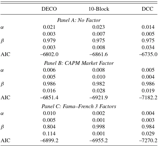
Table 3a. Full-sample correlation estimates for S&P 500 constituents, 1995–2008
DECO 10-Block DCC
Panel A: No Factor
α 0.021 0.023 0.014
0.003 0.007 0.005
β 0.979 0.975 0.975
0.003 0.008 0.034 AIC –6802.0 –6861.6 –6735.0
Panel B: CAPM Market Factor
α 0.006 0.008 0.005
0.005 0.010 0.004
β 0.986 0.982 0.986
0.016 0.028 0.019 AIC –6851.4 –6921.9 –7182.2
Panel C: Fama–French 3 Factors
α 0.010 0.002 0.004
0.005 0.001 0.003
β 0.804 0.998 0.984
0.114 0.001 0.029 AIC –6899.2 –6955.2 –7270.2
The table presents estimation results for nine dynamic covariance models. Each model is a two-stage quasi-maximum likelihood estimator and is a combination of one of three first-stage models with one of three second-first-stage models. The first-first-stage models are GARCH regression models imposing a factor structure for the cross section of returns, in which the structures are no factor (Panel A), the Sharpe–Lintner one-factor CAPM (Panel B), and the Fama–French (1993) three-factor model (Panel C). The second-stage correlation models, estimated on standardized residuals from the first stage, are one- and 10-Block DECO and composite likelihood DCC. Below each estimate, we report quasi-maximum likelihood asymptotic standard errors in italics. Asymptotic standard errors are calculated using the “sandwich” covariance estimator of Bollerslev and Wooldridge (1992). For each model, we report the Akaike information criterion calculated using the sum of the first- and second-stage log likelihoods penalized for the number of parameters in both stages. The analysis is performed on the S&P 500 dataset described in Section 4.
of individual stock returns on a set of factors where, as be-fore, all factors and idiosyncrasies are modeled as asymmet-ric GARCH(1,1). The second-stage is estimated with the basic DECO specification. Estimation results are shown in the first column of Panels B and C inTable 3(a). CAPM residual cor-relations are slightly less persistent than the no factor case, with ˆα+βˆ=0.992. Adding the market factor substantially in-creases the log-likelihood, even after accounting for its addi-tional parameters (as seen by the decreased AIC versus column 1 of Panel A). CAPM residual correlations are plotted against S&P 500 Index price level inFigure 2(b). On average, the resid-ual correlation is very low, dropping to less than 2% for most of the sample from a time average of over 20% with no factor (Figure 2(a)). The most striking feature of this plot is the large increase in residual correlations from 1999 through late 2001, corresponding to the rise and fall of the technology bubble. It appears that, before and after the tech boom, the CAPM does a very good job of describing return correlations. During the tech episode, an additional factor seems to surface. The impact of this factor on dependence among assets is not captured by the CAPM, but is picked up by residual DECO.
Estimates for residual correlations using the Fama–French three-factor model show much weaker dynamics among residual correlations, as persistence drops to ˆα+βˆ=0.814. Including three factors further improves the AIC.Figure 2(c) shows that residual correlations are almost always about 1.5% and flat. The
only exceptions are brief spikes to 3% during the peak of the tech bubble and the crisis of late 2008.
4.4 Comparing DECO and DCC Correlations
The previous subsections have explored DECO fits using no factor structure, the one-factor CAPM, and the Fama–French three-factor model. We now examine the fits of DCC for each of these three first-stage models to compare with DECO. DCC is estimated using composite likelihood with submodels that are pairs of stocks;nof the possiblen(n−1)/2 pairs are randomly selected as submodels, wheren=466 for our sample. The use of a large subset of all pairs reduces computation time while negligibly degrading the performance of the estimator (as sug-gested by Engle et al.2008). As a check of this point, we use all pairs for estimating composite likelihood DCC in a smaller cross-section of 36 Dow Jones constituents (a subset of our S&P sample) and find that the results are nearly identical to the results when only 36 randomly selected pairs are used.
DCC parameter estimates are shown in the third column of
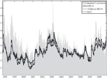
Table 3(a). When no factor is used, parameter estimates for DECO and DCC are similar and within two standard errors of each other. DECO achieves a lower AIC, making it the better model according to this criterion. Note, DECO and DCC use the same number of parameters, so the lower AIC for DECO is due solely to its better likelihood fit. We next evaluate how much pairwise DCC correlations deviate from the equicorrelation se-ries of DECO.Figure 3(a) plots DECO against the 25th, 50th, and 75th percentile of pairwise DCC correlations when the first stage model has no factor. These quartiles give a sense of the dis-persion of pairwise correlations. As the figure shows, the upper and lower quartiles are almost always within 5% of the me-dian, and the dynamic pattern of the quartiles closely track the equicorrelation. The similar correlation dynamics for pairs of stocks and for equicorrelation is consistent with DECO’s ability to achieve a superior fit.
When the first-stage model includes the CAPM market fac-tor, DCC α andβ estimates again are very close to those of DECO. In this case, DCC fits the data better according to the Akaike criterion. To understand how DCC might provide a bet-ter fit, consider the DCC residual correlation quartiles shown in
Figure 3(b). We see first that the dispersion of correlations has increased relative to the average correlation. Residual equicor-relation is roughly 2–3% over time, while the 75th and 25th DCC percentiles are around 6% and –3% on average. Further-more, other than during the technology bubble, there appears to be no systematic relationship between the time series pattern in equicorrelation and the pattern of pairwise correlations. This picture therefore suggests that the ability of DECO to describe residual CAPM correlations is limited, consistent with the AIC values we find.
Using the Fama–French model reinforces the notion that DCC is a more apt descriptor of factor model residuals due to the ten-dency for residual pairwise correlations to exhibit idiosyncratic dynamics. Table 3(a), Panel C shows that DCC continues to find stronger dynamics in correlations than DECO in terms ofα andβ estimates, and pairwise DCC correlations inFigure 3(c) are quite distinct from the equicorrelation in their time series
(a)
(b)
(c)
19950 1997 1999 2001 2003 2005 2007 2009 0.1
1995 1997 1999 2001 2003 2005 2007 2009 -0.04
1995 1997 1999 2001 2003 2005 2007 2009 -0.03
Figure 3. The figure shows fitted correlations of S&P 500 Con-stituents, 1995–2008. The figure shows fitted correlations of S&P 500 constituents estimated with DECO and DCC. Correlation fits are based on model estimates in Table 3. The graphs correspond to the follow-ing first-stage factor schemes: (a) no factor, (b) the Sharpe–Lintner CAPM, and (c) the Fama–French (1993) three-factor model. Each plot shows the fitted one-block equicorrelation and the 25th, 50th, and 75th percentile of pairwise DCC correlations in each period.
behavior. In summary, our results elucidate the conditions under which DECO can provide a good description of the data. When comovement among all pairs shows broadly similar time series dynamics, DECO fits well and outperforms DCC. Conversely, when dynamics in pairwise correlations are dissimilar, DCC may be a more appropriate model.
4.5 Block DECO
In our last description of correlations among S&P con-stituents, we repeat the above analyses using 10-Block DECO as the correlation estimator. Stocks are assigned to blocks based on SIC codes according to the industry classification scheme for Ken French’s 10 industry portfolios. We esti-mate 10-Block DECO using Gaussian composite likelihood with submodels that are pairs of blocks. Due to the low number of blocks, all 10(10−1)/2 pairs of industries are used to form the Block DECO composite likelihood. In par-ticular, when formulating the likelihood contribution of in-dustry pair i, j, a total of ni+nj stocks are used in the
submodel.
When no factors are used in the first-stage GARCH regres-sions, Block DECO achieves a better AIC than both DCC and DECO, and finds similar parameter estimates. To get a sense of the flexibility Block DECO adds to the correlation structure,
Figure 4plots within-industry correlations for energy, telecom, and health stocks. We choose only three of the 10 sectors to keep the plot legible while illustrating the richness a block structure can add to the cross-section of correlations. A few interesting patterns emerge. First, the correlation among energy stocks has slowly trended upward over the entire sample. While correla-tions were low for the market as a whole over 2004–2007, energy correlations remained high and continued to climb. Telecom stocks, meanwhile, had the sharpest rise in correlations in the market downturn following the technology boom. Health stocks maintained relatively low correlations throughout the sample. All three groups, however, experience drastic increases in cor-relations during late 2008, at which time all groups saw their highest level of comovement.
We also estimate Block DECO on residuals from the CAPM and Fama–French model. While Block DECO achieves a bet-ter fit than DECO in these factor models, DCC maintains the superior AIC. Block DECO, like DCC, finds more persistent dy-namics in correlations for Fama–French residuals than DECO.
4.6 Equicorrelation and Implied Correlations, Dow Jones Index
Options traded on an index and its members provide an oppor-tunity to validate fits from correlation models against forward-looking implied correlations that are based solely on options prices. We briefly compare fitted correlations from DECO and DCC to option-implied correlations. Since options do not ex-ist for all members of the S&P 500, we instead examine the Dow Jones Index, for which liquid options are traded on all constituents. Our sample of options data for the Dow Jones and its members begins in October 1997 (when Dow Jones Index options were introduced) through September 2008. Implied cor-relation is calculated from implied volatilities of the index and its constituents as in Equation (1). We use implied volatilities on call options standardized to have one month to maturity, avail-able from OptionMetrics. We also estimate DECO, 10-Block DECO, and DCC using daily returns on Dow Jones stocks from 1995–2008. The first-stage model in all cases has no factors. Estimates are reported inTable 3(b).Figure 5plots the implied correlation against the average fitted pairwise correlation of each
1995 1997 1999 2001 2003 2005 2007 2009 0.1
0.2 0.3 0.4 0.5 0.6 0.7 0.8
B
loc
k C
o
rr
el
ation
Energy Telecom Health
Figure 4. Selected block equicorrelations for the S&P 500, 1995–2008. The figure shows within-block equicorrelations of energy, telecom, and health stocks (according to the 10 industry assignments on Ken French’s website) in our S&P 500 sample. Estimates are made with Block DECO composite likelihood using a first-stage model with no factor. Correlation fits correspond to model estimates in Table 3.
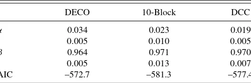
model. All three models broadly match the time series pattern of implied correlation. DECO seems to adjust more quickly and more dramatically during periods of sharp movements in the im-plied series. Imim-plied correlations are almost always higher than model-based correlations, representing the correlation risk pre-mium documented by Driessen, Maenhout, and Vilkov (2009).
4.7 Out-of-Sample Hedging Performance
One way to evaluate the performance of DECO and DCC in an economically meaningful way is to use out-of-sample covari-ance forecasts to form minimum varicovari-ance portfolios. A superior forecasting model should provide portfolios with lower variance
1998 1999 2000 2001 2002 2003 2004 2005 2006 2007 2008
0.1 0.2 0.3 0.4 0.5 0.6 0.7 0.8 0.9
Implied Correlation DECO
10-Block DECO DCC
Figure 5. Dow Jones index option-implied correlations and model-based average correlations. The figure shows the option-implied correlation of Dow Jones stocks and the average pairwise correlation estimated using DECO, 10-Block DECO, and DCC. Model-based correlations correspond to parameter estimates shown inTable 3(b). The options sample horizon covers October 1997 to September 2008, and the correlation model fits are estimated using data from January 1995 to December 2008.
Table 3b. Full-sample correlation estimates for Dow Jones constituents, 1995–2008
DECO 10-Block DCC
α 0.034 0.023 0.019
0.005 0.010 0.005
β 0.964 0.971 0.970
0.005 0.013 0.007
AIC –572.7 –581.3 –577.4
This table repeats the analysis of Table 3(a), Panel A (no factor) for the subsample of 36 Dow Jones constituents.
than portfolios formed based on competing models. This type of comparison is motivated by the well-known mean–variance optimization setting of Markowitz (1952). Consider a collection ofnstocks with expected return vectorµand covariance matrix
. Two hedge portfolios of interest are the global minimum variance (GMV) portfolio and the minimum variance portfolio subject to achieving an expected return of at leastq. The GMV portfolio weights are the solution to the problem
min
ω ω
′ω s.t.ω′ι
=1.
The MV portfolio is found by solving this problem subject to the additional constraintω′µ≥q. The expressions for optimal weights are
ωGMV =
1 A
−1ι
and
ωMV= C−qB
AC−B2
−1ι
+ qA−B AC−B2
−1µ,
(13)
whereA=ι′−1ι,B
=ι′−1µandC
=µ′−1µ.
We focus on two forecasting questions. The first is motivated by Elton and Gruber (1973), who demonstrated that minimum variance portfolio choices can be improved by averaging pair-wise correlations within groups. Our question extends this idea to the conditional setting, and is linked to the question of best correlation fit structure to employ with ex post averaging. Once DECO is estimated, it can be used to form out-of-sample unre-stricted pairwise correlation forecasts (as in DCC). These pair-wise correlations can then be used to form different fitted cor-relation structures by averaging pairwise corcor-relation forecasts within blocks as discussed in Section 2.4 and outlined in Fig-ure 1. Ultimately, DECO estimates can be used to construct cor-relation forecasts that are equicorrelated, block equicorrelated, or unrestricted. By varying the choice of correlation structure in our forecasts, we can evaluate the portfolio choice benefit of averaging pairwise correlations in a conditional setting (while keeping the estimation structure fixed as basic DECO).
Our experiment proceeds as follows. Using daily returns of the S&P cross-section for the five-year estimation window be-ginning in January 1995 and ending December 1999, we
1. Estimate first-stage factor volatility models for each stock 2. Use estimates of regression/volatility models to form
one-step ahead volatility forecasts for each stock
3. Using devolatized residuals from the first stage, estimate the second-stage correlation model
4. Use correlation model parameter estimates to forecast unre-stricted pairwise correlations one step ahead
5. Conduct ex post averaging of pairwise correlations to achieve each of the following correlation forecast fit structures (i) un-restricted, (ii) 30 industry blocks, (iii) 10 industry blocks, and (iv) a single block
6. Combine correlation forecasts for each fit structure with re-gression/volatility model estimates and forecasts to construct the full covariance matrix forecast
7. Plug the resulting covariance forecast into (13) to find opti-mal portfolio weights (this step also requires an estimate of mean return µ. We set µequal to the historical mean and chooseq=10% annually)
8. Record realized returns for portfolios based on forecasts.
One-step-ahead forecasts and portfolio choices are made in this manner for the next 22 days. After 22 days, the second-stage model is reestimated and the new parameters are used to generate the one-day ahead forecasts for the next 22 days and new out-of-sample portfolio returns are calculated. This is repeated until all data through December 2008 have been used. The result is a set of 2263 out-of-sample GMV and MV portfolio returns for each model.
After completing the forecasting procedure and recording portfolio returns, we calculate the realized daily variance for each ex post correlation fit structure. A superior model will pro-duce optimal portfolios with lower variance realizations. We can test the significance of differences between portfolio vari-ances for different correlation fit structures with a Diebold and Mariano (2002) test between the vectors of squared returns for each method. These tests are also related to the tests of Engle and Colacito (2006).
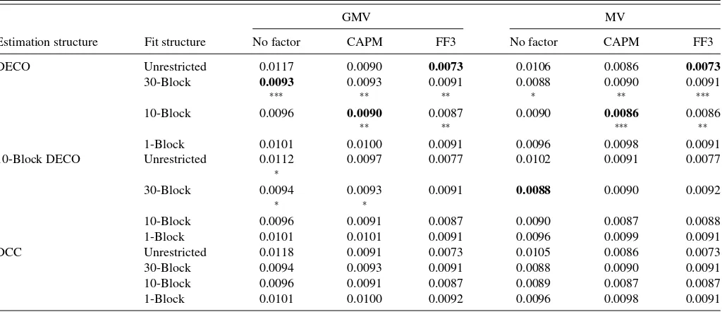
Out-of-sample GMV portfolio standard deviations when the first-stage has no factors model are reported in the first column ofTable 4. A 30-block fit structure generates the lowest variance GMV portfolio with a standard deviation of 0.0093. This im-proves over the next best ex post structure, which used 10 blocks and achieves a standard deviation of 0.0096. The difference is significant at the 0.1% one-sided significance level. The same result is found for MV portfolios.
We repeat the hedging experiment using the CAPM and Fama–French factor structures. When the CAPM is used, ex post averaging over 10 blocks takes over the lowest variance posi-tion, significantly outperforming the second best (unrestricted) structure at the 2.5% one-sided significance level. The 10-block fit structure also achieves the lowest variance MV portfolio, though its improvement is not statistically significant over the next best model. For the Fama–French model, the unrestricted fit becomes the superior structure and significantly outperforms (block) equicorrelated structures.
DECO’s minimum variance portfolio results so far suggest that there can be hedging benefits to varying the block struc-ture of correlations after estimation. These results, however, do not speak about the estimation ability of different correlation models. If the same exercises were repeated using different cor-relation models than DECO to estimateα andβ, how would portfolio choices fare?
Table 5reports the standard deviations of GMV and MV port-folios when 10-Block DECO and DCC are used for estimation.