Full Terms & Conditions of access and use can be found at
http://www.tandfonline.com/action/journalInformation?journalCode=ubes20
Download by: [Universitas Maritim Raja Ali Haji] Date: 12 January 2016, At: 23:52
Journal of Business & Economic Statistics
ISSN: 0735-0015 (Print) 1537-2707 (Online) Journal homepage: http://www.tandfonline.com/loi/ubes20
Modeling Parametric Evolution in a Random Utility
Framework
Jin Gyo Kim, Ulrich Menzefricke & Fred M Feinberg
To cite this article: Jin Gyo Kim, Ulrich Menzefricke & Fred M Feinberg (2005) Modeling
Parametric Evolution in a Random Utility Framework, Journal of Business & Economic Statistics, 23:3, 282-294, DOI: 10.1198/073500104000000550
To link to this article: http://dx.doi.org/10.1198/073500104000000550
Published online: 01 Jan 2012.
Submit your article to this journal
Article views: 63
Editor’s Note:
Zellner Prize for Best Thesis in Business and Economic Statistics.
Modeling Parametric Evolution in a Random
Utility Framework
Jin Gyo K
IMMIT Sloan School of Management, Cambridge, MA 02142 (jgkim@mit.edu)
Ulrich M
ENZEFRICKEJoseph L. Rotman School of Management, University of Toronto, Toronto, Ontario, Canada, M5S 3E6 (menzefricke@rotman.utoronto.ca)
Fred M. F
EINBERGUniversity of Michigan Business School Ann Arbor, MI 48109 (feinf@umich.edu)
Random utility models have become standard econometric tools, allowing parameter inference for individual-level categorical choice data. Such models typically presume that changes in observed choices over time can be attributed to changes in either covariates or unobservables. We study how choice dy-namics can be captured more faithfully by also directly modeling temporal changes in parameters, using a vector autoregressive process and Bayesian estimation. This approach offers a number of advantages for theorists and practitioners, including improved forecasts, prediction of long-run parameter levels, and cor-rection for potential aggregation biases. We illustrate the method using choices for a common supermarket good, where we find strong support for parameter dynamics.
KEY WORDS: Bayesian model; Choice model; Dynamic model; Logit model; Scanner panel data; Varying-parameter model; Vector autoregressive process.
1. INTRODUCTION
The modeling of sequential, individual-level choice has emerged as a research area of great breadth, with applica-tions throughout economics, statistics, psychology, and else-where. A fundamental goal is determining how choices evolve over time, and which variables drive them. A rich literature has emerged to aid researchers in linking exogenous covariates to temporal changes in choices. Because data are available on observed choices but not on unobserved measures of relative “attractiveness” of available options, the dominant method of achieving such a linkage has been through random utility mod-els (McFadden 1973; Manski 1977).
Within the random utility framework, one must specify both a utility and an error structure, as well as some link func-tion to convert to observables. Consequently, the lion’s share of research has been dedicated to those tasks. For example, prior approaches to modeling choice dynamics capture tempo-ral changes in individual-level utilities by introducing lagged terms for previous choices (cf. Heckman 1981) or by invoking a generalized stochastic error structure (e.g., Allenby and Lenk 1994, 1995). Although these models do capture some types of changes in utility over time in a systematic way, they do not consider changes in variable weights, and so amount to mod-eling shifts in the intercept of the deterministic component of utility.
We aim to demonstrate that an essential element of choice or utility dynamics can be captured by directly modeling changes in parameters. To that end, we propose a Bayesian dynamic logit model designed to capture choice dynamics by estimating a vector autoregressive process for the parameters of individu-als’ linear utility functions. Such an approach allows rigorous
investigation of a number of issues of interest in forecasting. First, can parameters be distinguished by whether they are time-varying? If they do evolve, can they be further distinguished by the nature of their evolution? And, most important for predic-tion, to what extent can understanding the nature of paramet-ric evolution be used to gain superior understanding of future choices? The model that we develop does indeed distinguish parameters along these lines, and uses that knowledge for im-proved forecasting.
The article is organized as follows. We review earlier litera-ture concerning parameter dynamics, specify a Bayesian model to account for them, and develop methods for its estimation. We then estimate the model on individual-level sequential choices, and demonstrate its in-sample and forecast performance. Fi-nally, we suggest possible sources for such dynamics, as well as potential extensions to the general method.
2. DYNAMIC MODEL SPECIFICATION
2.1 Previous Approaches to Changes in
Utilities Over Time
Although we are concerned with statistical issues, we note that numerous behavioral studies have suggested that parame-ters—as embodied by individual-level sensitivities—do indeed change over time. Research on preference reversals, for exam-ple, has demonstrated that the so-called “weight function” of
© 2005 American Statistical Association Journal of Business & Economic Statistics July 2005, Vol. 23, No. 3 DOI 10.1198/073500104000000550
282
attributes depends on such contextual features as scale patibility (Slovic, Griffin, and Tversky 1990), strategy com-patibility (Tversky, Sattath, and Slovic 1988), and framing (Kahneman and Tversky 1979; Thaler 1985). Decision weights are also known to be sensitive to the scale change of attribute values in an experimental setting (von Nitzsch and Weber 1993).
Previous statistical approaches to capturing utility change over time can be separated into two broad classes, depend-ing on whether intercept shifts are taken to be deterministic or stochastic. Most previous models that introduce lagged choice variables make use of a deterministic intercept shift; the lagged choice shifts the constant term of the deterministic component of the utility for any particular option, so that the intercept isα′=α+γDt−1, whereDt−1 is a dummy variable for the particular option, equaling 1 only if that option was chosen at timet−1. Typically, the effects of the lagged choice variables
γare assumed to be homogeneous across units and options. It is important to note that this approach can only capture intercept shifts (in utilities over time) in a deterministic way. In contrast, Allenby and Lenk (1994, 1995) developed a logistic regression model that updates utilities over time by introducing an autore-gressive error structure. In their model, the new interceptα′ is given byα+ρεt−1, where 0<|ρ|<1 andεt−1is the stochastic component of utility at timet−1. Clearly, neither of these ap-proaches can account for utility changes generated by a change in variable weights over time.
2.2 Observation and Evolution Densities
We describe the dynamic logit model and use three generic subscripts; h denotes an individual unit of observation (h=
1, . . . ,H),jdenotes an option (j=1, . . . ,J), andtdenotes time (t=1, . . . ,T). Letyht=jdenote the event that unithchooses optionjat timet,letxhjtdenote unith’sk-dimensional covari-ate vector for optionjat timet, and letuhjtdenote unith’s utility for optionjat timet. Thus
uhjt=β′htxhjt+εhjt, (1)
whereβht is a k-dimensional coefficient vector for unit h at timetandεhjtis an associated error. Ifεhjtis iid Gumbel, then a dynamic logit model arises for choice probability phjt (cf. McFadden 1973),
phjt=p(yht=j|βht)=
exp(β′htxhjt)
J
i=1exp(β
′
htxhit)
. (2)
To model parametric temporal variation, we assume that
βhtcan be decomposed into two parts,
βht=βt+bh, (3) whereβt is a time-varying coefficient vector common across units andbhis a vector of random effects to incorporate hetero-geneityacrossunits. Now (2) simplifies to
phjt=p(yht=j|βt,bh). (4)
To capture dynamics for βt, we introduce a vector autore-gressive process of order p, VAR(p) (see, Li and Tsay 1998; Lütkepohl 1991; Polasek and Kozumi 1996),
βt=d+
p
n=1
Anβt−n+wt [wt∼N(0,w),t=1, . . . ,T]
=d+AZt−1+wt, (5)
where d is a k-dimensional vector, An is a (k×k) coef-ficient matrix, A=(A1, . . . ,Ap) is a k×kp matrix, Zt =
(β′t, . . . ,β′t−p+1)′ is a kp-dimensional vector, and wt is a
k-dimensional white noise term.
Note that a number of common univariate and multivari-ate stochastic process models, such as random walk, random walk with drift, and AR(p), are special cases of (5). Because Anis not assumed to be diagonal, an advantage of the VAR(p) process over the popular dynamic simultaneous equations ap-proach is that it allows one to monitor the relationship between a particular element ofβtand a different element ofβt−n. Fur-ther, (5) can capture both stationary and nonstationary dynam-ics; it is well known that the VAR(p)process is stable and thus stationary if
det(Ik−A1l− · · · −Aplp)=0 for|l| ≤1, (6) that is, if there is no root within or on the unit disk of the reverse characteristic polynomial of the VAR(p)process. If the VAR process is stable, then the expected value ofβtdoes not depend ont, that is,
µβ=E(βt)=(I−A1−A2− · · · −Ap)−1d,
where the expectation is with respect towt,t=1,2, . . . (Lütke-pohl 1991).
Finally, we model the heterogeneity ofbhin (3) as a multi-variate normal random effect,
p(bh|b)=Nk(0,b) ∀h, (7)
wherebis an unknown covariance matrix.
2.3 Prior Distributions
Priors are required for {βt}0t=1−p, d,A, w, andb.
Fol-lowing standard assumptions of dynamic state-space models (Cargnoni, Müller, and West 1997; Carlin, Polson, and Stoffer 1992; Harrison and Stevens 1976; West and Harrison 1997), we assume that{βt}0t=1−p,d,A,w, andbare mutually
indepen-dent and use the following prior distributions:
p(βi)=Nk(m0,S0), wherei=1−p, . . . ,0; (8)
p(d)=Nk(md,Sd); (9)
p(vec(A))=Nk2p(mα,Sα); (10)
p(w)=IWk(vw,Sw); (11)
and
p(b)=IWk(vb,Sb). (12)
Here vec(·) is the usual column stacking operator, so that vec(A) is a k2p-dimensional vector. The expression p()=
IWk(v,S)denotes thathas ak-dimensional inverted Wishart
distribution with parametersvandS, wherev>0 andSis non-singular, that is, p()=IWk(v,S)∝||−(1/2v+k)exp(−12 ×
tr−1S). Furthermore, the parameters of the prior distributions (m0,S0,md,Sd,mα,Sα,vw,Sw,vb, andSb) are known
val-ues that we choose to obtain noninformative proper priors. In particular, for the prior of vec(A),we use the Minnesota pri-ors (Doan, Litterman, and Sims 1984; Litterman 1986), which are specialized for the VAR(p)process. Specifically, we choose mα=0andSαto be a diagonal matrix with elements ing diagonal elements ofw,λis the prior belief on the
tight-ness around 0 for the diagonal elements ofA1,and 0< θ <1 reflects the prior belief that most of the variation of βt is ex-plained by its own lags. Thus the Minnesota priors are locally noninformative proper priors around 0, an attractive property because, under the stability condition,Antends to shrink to 0 rapidly inn(cf. Lütkepohl 1991, p. 208). The Minnesota priors can also be characterized as smoothly decreasing priors over lags in a harmonic manner, which is also useful for order selec-tion ofp.
3. ESTIMATION AND MODEL CHOICE
We first discuss parameter estimation of the proposed dy-namic logit model, then describe the model selection procedure.
3.1 Full Posterior Distribution
Using the likelihood and prior specifications, we obtain the posterior distribution for all parameters. Let
• H= {1,2, . . . ,H}be the set of all individuals,
• Htbe a subset ofHthat consists of individuals that make
choices at timet, Then the posterior distribution is
p(β,b,d,A,w,b|y)
This posterior distribution has several sets of parameters, with numerous elements. Specifically, forβt(t=1−p, . . . ,T), there are k(p +T); for bh (h =1, . . . ,H), kH; for d, k; forA,k2p; and for bothwandb,12k(k+1). In the
forthcom-ing illustration, we haveH=492,T=90, andk=6, yielding 3,540+42pelements overall.
Because analytic methods to evaluate the posterior distrib-ution in (14) are not available, we use Markov chain Monte Carlo (MCMC) methods, as described in Section 3.2. For model selection and Bayesian hypothesis testing, we use Bayes fac-tors (Bernardo and Smith 1994) to compare two models (or hy-potheses)H1andH2, Bayes factor, we must evaluate the integrated likelihoods, using the results from the MCMC simulation. Let(g),g=1, . . . ,G, denote theGvalues of generated from the posterior distri-bution of,p(|H1).The integrated likelihood for model 1,
p(y|H1)=p(y|,H1)p(|H1)din (15), can be estimated by the harmonic mean estimator (Newton and Raftery 1994),
p(y|H1)=
This estimator converges almost surely to the correct value, but it does not generally satisfy a Gaussian central limit theorem. Nevertheless, it has been found to work reasonably well with large samples (cf. Kass and Raftery 1995).
3.2 Markov Chain Monte Carlo Sampler
To evaluate the posterior distribution, p(β,b,d,A,w,
b|y),given in (14), we implement a MCMC sampler, using
the following conditional posterior distributions:
p(β|b,d,A,w,b,y)
↔p(b|β,d,A,w,b,y)↔p(d|β,A,w,b,y)
↔p(A|β,b,d,w,b,y)↔p(w|β,b,d,A,b,y)
↔p(b|β,b,d,A,w,y).
We next describe the sampling procedure for each of these.
3.2.1 Sampling From p(β|b,d,A,w,b,y). To sample
fromp(β|b,d,A,w,b,y),we need the conditional
rior density forβt,p(βt|βm=t,b,d,A,w,b,y).When 1≤
Given (17), a Metropolis–Hastings algorithm step can be conducted as follows (Chib and Greenberg 1995; Metropolis, Rosenbluth, Rosenbluth, Teller, and Teller 1953):
1. Sampleβ∗t from a proposal density, N(βpret , φβI), where
βpret is the most recently updated value andφβis a fixed
tuning constant.
2. Substituteβ∗t forβpret with acceptance probability
π(β∗t,βpret )=min sity with meanFtft and covariance matrixFt, evaluated atβt. bpreh is the most recently updated value andφb is a fixed
tuning constant.
2. Substituteb∗hforbpreh with acceptance probability
π(b∗h,bpreh )=min
The conditional posterior density fordis
p(d|β,A,w,b,y)∝
By completing the square inα,
p(α| ˜β,w)=N(α∗,∗α), (19)
a (k2p)-dimension normal density with mean vector α∗ =
∗α{S−α1mα+(Z⊗w−1)β˜}and covariance matrix∗α= [S−α1+ (ZZ′⊗−w1)]−1.
If we do not impose the stability restriction on the VAR(p)
process, then (19) can be used directly to sampleα. In this case the probability of the VAR(p) process being stable can be esti-mated by counting the number of iterations when the sampledα
satisfies (6). However, with a stability restriction on the VAR(p)
process, there is a difficulty in samplingα. Under the stability condition (6),α should be sampled from N(α∗,α∗)I(α∈B), where B is the region in which the stability condition is sat-isfied. The simplest way to sample α under the stability re-striction is to use rejection sampling, by accepting αsampled from N(α∗,∗α)only if it satisfies (6). However, rejection sam-pling will be inefficient, because the rejection rate increases
exponentially with the dimension of α. Even for a univariate AR(p)process, the acceptance rate of rejection sampling ap-proaches 50% (e.g., Barnett, Kohn, and Sheather 1996).
We therefore sample α directly from N(α∗,∗α)I(α∈B)
under the stability restriction by using single-variable slice-sampling, as proposed by Neal (1997). Recall thatα=(α1, . . . ,
αk2p)′, and consider the conditional distribution of αi,f(αi)=
p(αi|remaining components of αi), which is proportional to N(α∗,∗α)I(α∈B). Generating values of αi proceeds by re-placing the previous value,αipre, with a new value,αinew, as fol-lows:
1. Define a horizontal slice,Sh= {αi:z<f(αi)}, wherezis an auxiliary variable sampled uniformly from(0,f(αipre)). 2. Find an interval,I=(L,R), aroundαprei onShsuch that
f(L) <zandf(R) <z.
3. Acceptαnewi , sampled uniformly fromI,iff(αinew) >z.
Roberts and Rosenthal (1999) showed that the slice sampler is irreducible and aperiodic and satisfies the detailed-balance condition. The advantages of the slice sampler are that it can be used for any log-concave probability density function. Fur-thermore, it can avoid slow random-walk convergence, because
αprei is always replaced byαinewin each iteration and it is pos-sible to obtain a large jump fromαipretoαnewi . Computation of
f(αi)involves the evaluation ofI(α∈B).Note that the eval-uation ofI(α∈B)does not require computation of lower and upper bounds of the regionB. One must simply check whether or notαifalls inside the regionB, by using (6).
In some cases, a researcher may have prior beliefs onα(or, equivalently,A) and so wishes to place restrictions on a subset ofα. In such a case,α, under arbitrary restrictions, can be eas-ily sampled as follows. Suppose thatα¯=(α′1;α′2)′withα2=a, whereais a vector of restricted values. Define a partition ma-trixPsuch thatα¯=Pα. Then the conditional posterior density ofα1givenα2=a, N(α1|α2=a),can be easily obtained from N(Pα∗,P∗αP′).If the partitioned submatrix forα2inP∗αP′
is singular, the Moore–Penrose inverse can be used to derive N(α1|α2=a).
3.2.4 Sampling From p(w|β,b,d,A,b,y)and p(b|β,
b,d,A,w,y). The conditional posterior density forwis
p(w|β,b,d,A,b,y)=p(w|β,{β}0m=1−p,d,A,y)
∝IW(v∗w,S∗w),
an inverted Wishart density withv∗w=vw+T andS∗w=Sw+
T
t=1ltl′t,wherelt=βt−d−AZt−1. The conditional posterior density forbis
p(b|b)=p(b|y,β,b,d,A,w,y)
∝IW(v∗b,S
∗
b), (20)
an inverted Wishart density withv∗b=vb+HandS∗b=Sb+
h∈Hbhb′h.
3.3 Comparative Model Specifications
The model (2) has parameters{βt}Tt=1,{bh}hH=1,d,{An}pn=1,
w, andb. We consider several alternative models that differ
by the structural assumptions imposed ond,{An}pn=1, andw,
as follows:
Model d {An}pn=1 w No parameter dynamics
M0: Static random-effects logit model NR 0 0 Parameter dynamics
M1: Dynamic linear model; random walk 0 p=1;A1=I NR M2: Random walk with a drift NR p=1;A1=I NR
M3: VAR(p) NR NR NR M4: Restricted VAR(p); RVAR(p) NR An= diagonal NR
NOTE: NR, no restriction.
All models listed in this table incorporate heterogeneity as a random-effects specification; see (7). Model M0 is the tra-ditional random-effect logit, which assumes that there are no parameter dynamics. ModelsM1–M4allow for parameter dy-namics in different ways. ModelM1, the popular dynamic linear model (Harrison and Stevens 1976; West and Harrison 1997), assumes a random-walk process forβt with mean vectorβt−1
and covariance matrixw. ModelM2assumes a random-walk process with a drift term for βt. Model M3 is the proposed VAR(p) process model. Model M4 is a restricted VAR(p) [RVAR(p)] process model under the restriction that{An}are diagonal matrices. Thus, in terms of parametric restriction,
M1⊂M2⊂M4⊂M3.
M0 can be easily estimated by skipping the MCMC steps forβt,w,and vec(A).M1 can be estimated by skipping the MCMC steps of d and vec(A). Similarly, M2 can be esti-mated by skipping the MCMC step for vec(A). We estimate
M3andM4under the stability condition given in (6).
To test the accuracy of parameter recovery, we performed two extensive simulation studies that differed in the relative com-plexity ofβt’s dynamics. All model parameters were recovered well in each. (Full results are available from the authors.)
4. EMPIRICAL ILLUSTRATION
4.1 Data and Independent Variables
The proposed model was estimated on A. C. Nielsen liq-uid detergent scanner data over 96 weeks. The data con-sist of 492 individual units (households) that made choices among four options{A,B,C,D}at least seven times during the 96-week period. The first 90 weeks of data were used as a train-ing sample to estimate the model, and the remaintrain-ing 6 weeks of data were used for predicting the future model parameters. The numbers of observations for the training and future parameter forecasting samples were 6,364 and 318. To ensure identifiabil-ity, the time-varying common effect of the fourth option as well as its random effect were fixed to be 0. This requires that the valuesxhjtfor optionjbe thedifferencesof the corresponding predictor variable values for optionsjand the base option,J. The vectorxhjtthus consists of three option dummies and three covariates, the differences in feature, display and price; note that the first two are binary, whereas the last one is continuous. All mean vectors of the normal priors [i.e.,m0,md, andmα
in (8) to (10)] were set to 0. The chosen values forS0 andSd
were 100I. For the inverse-Wishart priors ofw andb, the
degree of freedom parameters were set at 2 and the scale pa-rameters were chosen so as to make the expected values 100I. For the value ofSαin (10) and (13), Litterman (1986) suggested
choosingλ,θ, and{σi}by examining the data and trying several different values. However, this approach entails double usage of data. We thus setλ=1.0,θto .5, and all ratiosσr/σcto 1. For VAR(p) whenp>1, we setSαusing (13) withλ=1.0,θ=.5,
andσr
σc =1.
4.2 Markov Chain Monte Carlo Estimation
The tuning constants for the proposal distributions in the Metropolis–Hastings algorithms (e.g.,φβ in Sec. 3.2.1) were
chosen to produce similar acceptance rates across models. There exists a trade-off between convergence speed and ac-ceptance rate in the Metropolis–Hastings algorithm (Chib and Greenberg 1995). As tuning constants become smaller, the ac-ceptance rate increases, but we need a longer chain, because the distance between the previous value and a newly accepted value becomes smaller. The chosen tuning constants for βt and bh were approximatelyφβ=.07 andφb=.3. For all models, the
acceptance rates for βt and b, given these tuning constants, ranged from 53.2% to 55.7% and from 53.8% to 57.5%.
The number of quantities of interest for the VAR(p)model is quite large. For example, excludingb, there are 630 quantities for the full VAR(1) model. Thus we must be careful in deter-mining convergence of the MCMC sampler. Specifically, we determine convergence after examining all quantities exceptb. To monitor convergence, we use Geweke’s (1992) convergence diagnostic, which is based on the smooth spectral density of a MCMC posterior sample. The periodogram for spectral density estimation involves two important choices: window and trunca-tion point. We use the Tukey window and choose the truncatrunca-tion point after looking at the autocovariance function, as Jenkins and Watts (1968) suggested.
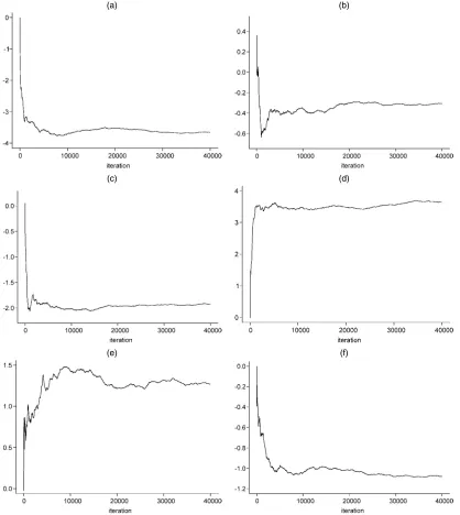
After 20,000 iterations, all models seem to reach conver-gence. Figure 1 is a typical example; for the VAR(1) model, it shows the trace plot for the six elements ofβ1for the first 40,000 iterations, where G represents Geweke’s convergence diagnostic with 20,000 burn-in periods. Across all models, the proportion of quantities that pass the Geweke diagnostic ranges from 91.3% to 98.1%. For the rejected quantities, we used Heidelberger and Welch’s (1983) half-width test, which the ma-jority passed. All inferences made here are based on the next 20,000 iterations.
4.3 Tests for Parameter Dynamics
After estimating modelsM0–M4, we can test whether there is evidence that parameters are time-varying. Specifically, we have the following hypotheses:
H1 : Parameters are static(M0) and
H2 : Parameters display some form of dynamics(M1,M2,M3, orM4).
The computed integrated likelihoods and the Bayes factors for a comparison of models M0 andMi (BFM0,Mi) are given
in Table 1. Because VAR(2) has a smaller integrated likelihood than VAR(1) and its estimatedA2is close to a null matrix, we do not estimate VAR(p) models of higher orders. We also do not estimate RVAR(p) with order greater than 2, because RVAR(2) shows smaller integrated likelihood than RVAR(1), and its esti-matedA2is close to null.
As shown in Table 1, we find exceptionally strong evidence supporting parameter dynamics. All models incorporating pa-rameter dynamics (M1–M4) are decisively preferred over the traditional static random-effects model (M0). Therefore, the model parameters, taken as a set, are evidently time-varying.
Selection Among Dynamic Models. The most preferred
among the parameter dynamics models (M1–M4) is RVAR(1), as shown in Table 1. The Bayes factors for RVAR(1) against the other dynamic models range from 9.8e+9 to 9.3e+15. Most interestingly, the RVAR(1) model is decisively preferred to the full VAR(1) model (Bayes factor=.98e+10), suggesting that A1is diagonal or very nearly so. Further, the VAR(1) and RVAR(1) models are preferred overM1andM2, implying that the matrixA1is not an identity matrix; furthermore, the value ofA1, reported later, suggests stable parameter dynamics.
4.4 Cross-Validation
One can appeal to cross-validation to compareM0, the static random-effects model, with the RVAR(1) model. To do this, we divide the 96 weeks of data into two sets. The “calibration data set” consists of the firstwweeks of data and is used for parame-ter estimation, whereas the “prediction dataset” consists of the remaining 96−w weeks and is used, unsurprisingly, for pre-diction. We investigated values for w= {50,55,60,65,70}to assess how additional calibration data affects predictive accu-racy. For the calibration dataset, we computed the Bayes factor of M0 versus RVAR(1). Results are given in Table 2. Regard-less of the value forw, model RVAR(1) is decisively preferred toM0.
The results for the prediction dataset were based on the fol-lowing approach. For both models M0 and RVAR(1), we es-timated the likelihood for the prediction data set as follows. For model M0, we estimated this likelihood by first comput-ing choice probabilities (2) for the prediction dataset (given bh and β simulated at each MCMC iteration) and taking an average of these choice probabilities for the prediction dataset across MCMC iterations. For model RVAR(1), we did the same given each value ofbhandβt,t=w, . . . ,96.
The resulting estimated log-likelihoods are also given in Ta-ble 2. The RVAR(1) model is moderately preferred to model
M0, so we next investigate RVAR(1) in more detail.
4.5 Estimation for the Training Sample
Because the RVAR(1) model performs better than other VAR(p) models (see Table 1), we report further estimation re-sults for this model alone. The RVAR(1) model implies the fol-lowing structure for the regression parameter vectorβht:
βht=βt+bh,
βt=d+A1βt−1+wt,
(a) (b)
(c) (d)
(e) (f)
Figure 1. Running Mean Plot ofβ1for the Full VAR(1) Model. (a) dumA(G= −.23); (b) dumB(G=1.15); (c) dumC (G=.34); (d) feature (G= −1.54); (e) display (G=1.17); (f) price (G= −.59). G denotes Geweke’s convergence diagnostic.
Table 1. Model Comparison for Training Sample
Log of integrated Bayes factor Mi likelihood ( BFM0,Mi)
No parameter dynamics case
M0: Static random-effects logit model −3,436.33 1.0 Parameter dynamics case
M1: Dynamic linear model −3,068.50 1.79e−160
M2: Random walk with a drift −3,072.44 9.22e−159
M3: VAR(p)
VAR(1) −3,061.90 2.44e−163 VAR(2) −3,075.66 2.31e−157
M4: RVAR(p)
RVAR(1) −3,038.89 2.48e−173 RVAR(2) −3,063.15 8.51e−163
and
bh∼N(0,b), wt∼N(0,w),
where A1 is a diagonal matrix. The parameters, apart from
βtandbh,are thusd, diag(A1),w, andb.
An important derived parameter is the long-run mean ofβt,
µβ=(I−A1)−1d. Furthermore, the long-run variance for the
ith element ofβtis
σβ2,i= w,i,i
1−A21,i,i, (21)
where w,i,i and A1,i,i are the ith diagonal elements of w
andA1. (See Hamilton 1994 for derivation of the moments of the full VAR(p) process.) An indication of the overall
Table 2. Cross-Validation Comparisons
Calibration sample Log-likelihood for prediction sample
log(integrated likelihood) Bayes factor
(H1: M0)
Data used M0 RVAR(1) M0 RVAR(1)
Weeks 1–50 −2,048.60 −1,782.73 3.42e−116 −2,256.17 −2,236.09 Weeks 1–55 −2,247.86 −1,946.93 1.33e−123 −1,942.92 −1,916.08 Weeks 1–60 −2,449.33 −2,166.87 2.13e−123 −1,623.90 −1,613.33 Weeks 1–65 −2,571.30 −2,315.47 7.84e−112 −1,396.55 −1,388.50 Weeks 1–70 −2,812.06 −2,516.53 4.50e−129 −1,080.21 −1,071.03
ity for elementiofβhtis thus given by var(βht,i)=
w,i,i
1−A21,i,i+b,i,i, (22)
which can be used to give an idea of the relative contributions of parameter dynamics and heterogeneity. It can also be compared with the elements ofE(βht)=µβ=(I−A1)−1dto get an idea of the relative variability of the elements ofβht.
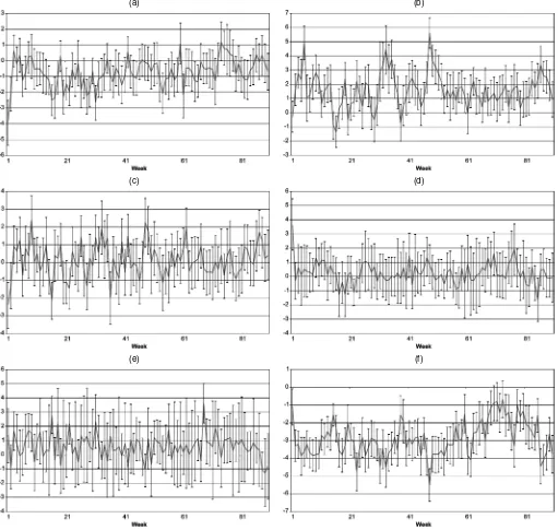
Estimation of βt. Figure 2 plots posterior means and the 5th and 95th percentiles for all time-varying parametersβt. It suggests fairly large temporal fluctuations; all intercepts show strong stochastic patterns, and all variable coefficients display stochastic dynamics. There are several periods that show sub-stantial shifts fromβt−1toβt.
Estimation of d and A1. If we define “significant differ-ence” to mean that a (5th percentile, 95th percentile) interval does not contain 0, Table 3 suggests that all elements ofd, ex-cept the coefficients of the dummy for option C (dumC) and of feature, are significantly different from 0. Likewise, the ele-ments ofA1corresponding to dumA, dumB, and Price are sig-nificantly different from 0, which suggests systematic dynamics over time for the corresponding elements ofβt.
Estimation ofw. Table 4 gives estimates forw.
Poste-rior means are given on and below the main diagonal, with posterior standard deviations given in parentheses; the poste-rior means of the correlation coefficients are given above the main diagonal. For the diagonal elements ofw, the ratios of
posterior means to posterior standard deviations are between 4.8 and 6.1. Thus, these elements ofwdiffer from 0,
imply-ing that all elements ofβtare changing over time. Among the off-diagonal elements, the coefficient of dumBhas meaningful correlation with the coefficient of dumAand the coefficient of price. Overall, we conclude that in our dataset,βtis apparently time-varying, with a fairly pronounced degree of white noise.
Estimation ofb. Table 5 gives estimates forb.
Poste-rior means are again given on and below the main diagonal, with posterior standard deviations in parentheses; the posterior means of the correlation coefficients are given above the main diagonal. This table suggests thatb is neither a null matrix
nor a diagonal matrix; furthermore, all diagonal elements are significantly different from 0.
Let us briefly examine the effect of parameter dynamics on the heterogeneity distribution by comparing posterior means for the covariancebfor both the RVAR(1) model and modelM0.
For modelM0, the posterior mean for the diagonal ofbis
5.4701 8.4474 11.1818 1.8029 1.9395 5.3011
(.6615) (.9838) (1.4515) (.2342) (.2695) (.6255)
,
where the respective posterior standard deviations are given in parentheses. These diagonal elements are 18.2–32.0% smaller than the corresponding elements ofbfor the RVAR(1) model,
which were given in Table 5. Therefore, the traditional random-effects logit model “underestimated” the extent of heterogene-ity.
Discussion. The elements of d and A1 for the option C dummy are essentially 0, but the corresponding variance inw
is positive. Thus the dynamics for the dummy variable of op-tion C consist of a white noise term only. The dynamics for the dummies for options A and B, on the other hand, consti-tute AR(1) processes. Allenby and Lenk (1994) also reported an autocorrelated error structure for utilities. Because they in-troduced a scalar for the error autocorrelation of utilities across choice occasions, they implicitly assumed that choice dummy effects would follow the same type of stochastic process with the sample autocorrelation coefficient. However, our results suggest different stochastic processes for each. Specifically, the feature coefficient seems to follow a pure white noise process, the Display coefficient is found to follow a white noise process with a non-0 mean, and the Price coefficient appears to follow a AR(1) process, over the observation period.
Table 6 gives the posterior means for the following quanti-ties:
• µβ, the long-run mean of βht (and the posterior standard deviation ofµβ)
• var(βht,i)=
w,i,i
1−A2 1,i,i
+b,i,i, an overall standard
devi-ation forβht
• b,i,i, the standard deviation of the heterogeneity com-ponent,bh, ofβht
• σβ,i=
w,i,i
1−A21,i,i, the long-run standard deviation of the dy-namic component,βt, ofβht
• w,i,i, the standard deviation of the “white noise” com-ponent ofβt.
The posterior mean ofµβdisplays the anticipated signs. The posterior standard deviations for some of the elements are rela-tively large, notably for the optionCdummy, Feature, and Dis-play, suggesting a fair amount of uncertainty about the actual value of µβ. A comparison of the results for µβ with those fordin Table 3 shows a moderate difference for Price.
The overall variability inβht, as measured by the posterior mean for the standard deviation var(βht,i), is quite large. In fact, all of these standard deviations arelargerthan the corre-sponding elements ofµβ, so the corresponding regression coef-ficients are negative for some households and time periods and positive for others. Thus, although the posterior means for the
(a) (b)
(c) (d)
(e) (f)
Figure 2. Dynamics ofβt. (a) dumA; (b) dumB; (c) dumC; (d) feature; (e) display; (f) price. Solid lines denote estimated values. The lower and upper bars denote the 5th and 95th percentiles.
elements of the long-run meanµβdisplay the anticipated signs, this is not necessarily true for individual households.
Let us next examine the contribution to the overall variabil-ity in βht that can be attributed to household heterogeneity and to parameter dynamics. Household heterogeneity can be measured by the square root of the diagonal elements of b,
b,i,i, and parameter dynamics can be measured by σβ,i=
w,i,i/(1−A21,i,i); see (21). Table 6 suggests that, except for Feature and Display, the posterior means for the standard de-viation of the heterogeneity component are quite a bit larger than the posterior means for the corresponding values ofσβ,i. Household heterogeneity is thus a very important component in the overall variability inβht.
Finally, let us contrastσβ,i, the long-run standard deviation of the dynamic component,βt=d+A1βt−1+w, with
w,i,i, the standard deviation of the “white noise” component,wt. The value of the posterior mean forw,i,iis only slightly smaller than that forσβ,i. This suggests that the “white noise” compo-nent is the dominant force in the parameter dynamics of each component ofβt.
4.6 Tests for Structural Change
It is important to check whether or not parameter dynamics truly exist in the training sample. After dividing the 90 weeks of data into nine datasets such thaty¯z= {yt}t10=z10(z−1)+1, wherez= 1, . . . ,9, we estimate all nine regression coefficients { ¯βz}9z=1
Table 3. Estimates of d and A
Estimate (5th percentile, 95th percentile) (standard deviation; MC error) interval
d
dumA −.5410 (.2265; .0094) (−.9182,−.1744) dumB 1.1811 (.3020; .0157) (.6867, 1.6780) dumC .1172 (.2900; .0168) (−.3634, .5982) Feature .1887 (.2213; .0107) (−.1722, .5536) Display .6387 (.3528; .0182) (.1115, 1.2451) Price −2.0741 (.4470; .0243) (−2.7682,−1.3043) diag(A1)
dumA .2322 (.1339; .0051) (.0282, .4632) dumB .2640 (.1397; .0058) (.0467, .4989) dumC −.0087 (.1525; .0067) (−.2328, .2655) Feature .1659 (.1691; .0134) (−.1411, .4213) Display −.0765 (.1890; .0089) (−.3999, .2241) Price .2958 (.1423; .0068) (.0747, .5420)
Table 4. Estimate ofΣw
dumA dumB dumC Feature Display Price
dumA 2.2014 .1842 .1582 −.0107 −.0581 .0797 (.3718)
dumB .4612 2.8483 .3099 −.0106 −.1046 −.2411 (.3033) (.5006)
dumC .3771 .8401 2.5797 .0145 −.0876 −.2210 (.2864) (.3567) (.4453)
Feature −.0249 −.0280 .0364 2.4485 .0129 .0094 (.2816) (.3243) (.3059) (.4502)
Display −.1580 −.3238 −.2581 .0371 3.3642 .0715 (.3433) (.3942) (.3784) (.3661) (.6998)
Price .1756 −.6038 −.5267 .0218 .2000 2.2031 (.2596) (.3089) (.2931) (.2783) (.3354) (.3630)
Table 5. Estimate ofΣb
dumA dumB dumC Feature Display Price
dumA 7.2242 .1683 .2161 −.1588 −.0699 −.0151 (.8232)
dumB 1.5397 11.5826 .2263 −.0486 −.1414 −.4943 (.7671) (1.3067)
dumC 2.3549 3.1222 16.4344 −.0314 −.1346 −.2889 (.9208) (1.1404) (2.0409)
Feature −.6407 −.2483 −.1913 2.2548 −.0736 .0311 (.4182) (.5370) (.6885) (.3371)
Display −.2898 −.7423 −.8419 −.1706 2.3795 .1282 (.4220) (.5843) (.7388) (.2292) (.3906)
Price −.1034 −4.2839 −2.9822 .1189 .5036 6.4841 (.5319) (.7081) (.7751) (.3935) (.4069) (.7261)
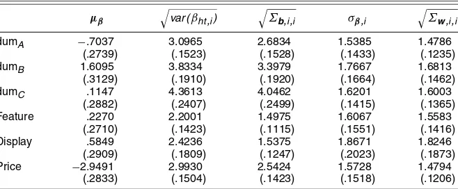
Table 6. Elements of Variation inβht
i µβ
var (βht,i)
Σb,i,i σβ,i
Σw,i,i
dumA −.7037 3.0965 2.6834 1.5385 1.4786 (.2739) (.1523) (.1528) (.1433) (.1235) dumB 1.6095 3.8334 3.3979 1.7667 1.6813
(.3129) (.1910) (.1920) (.1664) (.1462) dumC .1147 4.3613 4.0462 1.6201 1.6003
(.2882) (.2407) (.2499) (.1415) (.1365) Feature .2270 2.2001 1.4975 1.6067 1.5583
(.2710) (.1423) (.1115) (.1551) (.1416) Display .5849 2.4236 1.5375 1.8671 1.8246
(.2909) (.1809) (.1247) (.2023) (.1873) Price −2.9491 2.9930 2.5424 1.5728 1.4794
(.2833) (.1504) (.1423) (.1518) (.1206)
for these nine datasets simultaneously, whereβ¯zcontains logit coefficients belonging toy¯z. As before, to estimate{ ¯βz}9z=1, we use the MCMC sampler; specifically, distributions involvingβ
in (14) are changed to estimate{ ¯βz}9z=1as follows: 9
z=1
p(y¯z| ¯βz,b)
p(β¯z). (23)
It is readily apparent that the foregoing model is a counterpart to the tests on structural intercept and slope changes in the clas-sical econometrics literature. Hence we call (23) a structural changemodel. By estimating this model, we can test
H1:β¯1= · · · = ¯β9 (M0) and
H2:β¯1= · · · = ¯β9 (structural change model). The log of the integrated likelihood of the structural change model is−3,351.46. Clearly, the null hypothesisH1is rejected (Bayes factor favoring H1over H2=1.38e−37). This in turn further verifies that parameter dynamics exist for these data. Note that the RVAR(1) model is still decisively preferred over the structural change model [Bayes factor favoring RVAR(1) over the structural change model=5.59e+135], implying that
βtvaries within each set of observations.
4.7 Aggregation Bias
The estimation results of the structural change model raise an issue. Typically, a researcher uses a subset of the entire avail-able data for model estimation purposes. However, the assump-tion that informaassump-tion obtained from currently available data will also be valid in the future may be problematic; furthermore, ob-tained estimates can depend on the time periods for which a choice model is fitted. Thus if parameter dynamics exist, then estimates deriving fromM0can suffer from aggregation bias.
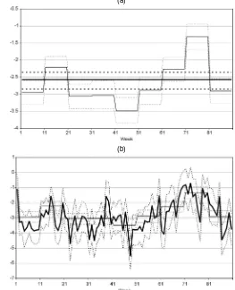
To illustrate the potential for aggregation bias, we compare the estimates of the structural change model with those of both
M0and RVAR(1). As shown in Figure 3, there are several cases in which the estimates of M0 deviate noticeably from the es-timates of the structural change model. However, the eses-timates of RVAR(1) strongly overlap with those of the structural change model. This suggests that it may be possible to substantially re-duce the degree of aggregation bias if parameter dynamics are appropriately accounted for.
4.8 Effects of Parameter Dynamics on Choice Behavior
We have shown that by incorporating temporal variation in parameters directly, choice dynamics can be better captured through a form of VAR process than by either the traditional static model or previous dynamic models. To examine poten-tial sources of superior prediction of choice dynamics, we now investigate the effects of exogenous covariates and parameter dynamics on choice behavior.
From (2), define the following derivatives:
ρxh
t,k(j,i)= ∂phjt
∂xhit,k
, ρβh
t,k(j)= ∂phjt
∂βt,k
,
and
ρxh
t,kβt,k(j,i)=
∂2phjt
∂xhit,k∂βt,k
.
(a)
(b)
Figure 3. Comparison of Price Coefficient Estimates for the Struc-tural Change ( ) and RVAR(1) ( ) Models. (a) Structural change ver-sus M0; (b) structural change versus RVAR(1). Lower and upper dotted lines enveloping each solid line of estimates denote the corresponding 5th and 95th percentiles.
Next, we computed ρxt,k(j,i)=
1
nt
h∈Htρxht,k(j,i) as the
sample average ofρxh
t,k(j,i)in periodt, wherent is the sample
size ofHt. Similarly, we computed the following sample aver-ages of the foregoing quantities:ρxt,k(j,j),ρβt,k(j),ρxt,kβt,k(j,j),
andρxt,kβt,k(j,i). For M0,βt,k is replaced by thekth element
of the regression coefficients. We compute these sample aver-age estimates for bothM0 and RVAR(1) for each time period. For optionj=A and variable=Price (k=6), Table 7 gives the MCMC estimates of these household-averaged derivatives further averaged over the 90-week observation period, for ex-ample,ρ¯xt,k(j,i)=
1 90
90
t=1ρxt,k(j,i). The pattern of results
in-dicates thatM0tends to overestimate all quantities of interest. 4.9 m-Step-Ahead Parameter Forecasting
Let us now consider forecasting. Given that we have data through period T, m-step-ahead forecasts can be readily ob-tained with another MCMC run. For example, such a simulation yields posterior distributions forβT+m.
We conducted six-step-ahead forecasting, obtaining poste-rior distributions forβT+m,whereT=90 andm=1, . . . ,6. At each MCMC iteration, it is straightforward to simulate these fu-ture parameters,βT+m, givenβ,d,A1, andw, using (5). The
posterior means and standard deviations of βT+m are, there-fore, readily available from MCMC runs ofβT+m. Table 8 gives
Table 7. The Averaged Effects of Covariate and Parameters on Choice Behavior
M0 RVAR(1)
¯
ρxt,k(A,A) −.1515 (.0047) −.1408 (.0052) ¯
ρxt,k(A,B) .0616 (.0028) .0556 (.0030) ¯
ρxt,k(A,C) .0333 (.0021) .0324 (.0023) ¯
ρxt,k(A,D) .0565 (.0027) .0528 (.0028) ¯
ρβt,k(A) −.0461 (.0015) −.0383 (.0013) ¯
ρβt,k(B) .0404 (.0015) .0327 (.0013) ¯
ρβt,k(C) .0227 (.0012) .0191 (.0011) ¯
ρβt,k(D) −.0170 (.0013) −.0135 (.0011) ¯
ρxt,kβt,k(A,A) .0559 (.0023) .0447 (.0022) ¯
ρxt,kβt,k(A,B) −.0151 (.0014) −.0119 (.0013) ¯
ρxt,kβt,k(A,C) −.0110 (.0012) −.0087 (.0011) ¯
ρxt,kβt,k(A,D) −.0298 (.0011) −.0241 (.0011)
NOTE: Standard deviations are in parentheses.
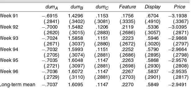
their means and standard deviations for weeks 91–96, suggest-ing considerable forecastsuggest-ing uncertainty.
We compared the performance of the six forecasted βT+m
values based on the RVAR(1) model with that of the tradi-tional static logit modelM0. For both models, we computed log-likelihood values for the prediction dataset. We obtained these likelihood values by first computing predicted choice probabil-ities, (2), for the forecasting dataset given all parameters simu-lated at each MCMC iteration, then taking the average of these predicted choice probabilities across MCMC iterations. The computed log-likelihoods for the forecasting sample, the sum-mation of log of (2) given the average of choice probabilities, are−202.21 for RVAR(1) and−208.89 forM0. For the future parameter forecasting sample, RVAR(1) demonstrates slightly better performance thanM0.
5. CONCLUSION AND FUTURE RESEARCH
Although choice models have achieved a great deal of so-phistication over the past decade, researchers have only recently begun to address the interplay of choice dynamics and parame-ter dynamics. To this end, we have proposed a general VAR framework to account for the phenomenon, one that can be grafted onto any specifications for utility or error structure. In this framework, we can rigorously test a number of hypothe-ses about the nature of parametric evolution—among them its
order, which parameters are involved, and which affect others— as well as demonstrate improved predictive performance.
A number of clear conclusions emerge from our empirical analysis. First and foremost, some (although not all) of the parameters demonstrated strong evidence of temporal varia-tion. This was clear even under the parsimonious specification that emerged as the strongest candidate, RVAR(1). Incorporat-ing such a stochastic parametric structure into existIncorporat-ing models would entail a comparatively modest increase in the number of estimated quantities, and should emerge as an attractive al-ternative to models presuming parametric constancy. Second, forecast performance was improved substantially over the stan-dard random-effects logit model. In fact, the random-effects model appears prone to aggregation biases when its parame-ter estimates deviate from the implied long-parame-term levels sug-gested by the VAR(p) specification. To our knowledge, this result is new, and we believe that it merits study in and of it-self, given the popularity of the random-effects logit model-ing framework. Finally, our data suggest that choice dynamics may be misattributed to exogenous covariates when parameters are presumed not to have dynamics of their own. For exam-ple, the random-effects model appears to underadjust for brand-switching behavior, perhaps because such behavior is assumed to be governed by external stimuli, given fixed parameters.
With respect to possible explanations for parameter dynam-ics, a number of potential explanations can be ruled out— specifically, systematic changes in the characteristics of pooled samples over time and changes in the distribution of stimuli across options. Further, analytic examination and simulation demonstrated that if all or some of the population update their parameters over time, then systematic parameter dynamics may exist even at the population level, as captured by the VAR(p) process.
Suggesting explanations for parametric evolution post hoc, other than those already tested, amounts to speculation. Some authors, however, have provided bases for further investiga-tions along these lines. Yang, Allenby, and Fennell (2002) noted that scanner panel data do not accommodate the proper unit of analysis in modeling preference changes: a person-activity oc-casion. They discussed how for many activities (e.g., snacking, serving wine), the consumer environment is not constant from one usage occasion to another, so that preferences are rightly situationally or motivationally dependent. Although they ex-plicitly pointed out that occasions for use of laundry detergent,
Table 8. Six-Step-Ahead Forecasting ofβt
dumA dumB dumC Feature Display Price
Week 91 −.6915 1.4296 .1153 .1756 .6704 −3.1938 (.2841) (.3402) (.3081) (.3335) (.4910) (.3367) Week 92 −.7000 1.5482 .1206 .2119 .5336 −3.0395
(.2620) (.3015) (.2883) (.2686) (.3057) (.2871) Week 93 −.7024 1.5858 .1151 .2223 .5946 −2.9868
(.2671) (.3037) (.2880) (.2672) (.3020) (.2797) Week 94 −.7032 1.5993 .1151 .2252 .5790 −2.9664
(.2705) (.3074) (.2881) (.2686) (.2895) (.2798) Week 95 −.7035 1.6048 .1147 .2263 .5868 −2.9576
(.2721) (.3097) (.2881) (.2698) (.2930) (.2808) Week 96 −.7036 1.6072 .1147 .2267 .5837 −2.9535
(.2729) (.3110) (.2881) (.2703) (.2901) (.2817) Long-term mean −.7037 1.6095 .1147 .2270 .5849 −2.9491
NOTE: Standard deviations are in parentheses.
the product class used in our study, are less likely to be subject to this sort of temporal preference variation, we believe that their approach merits formal study on data like our own, which would provide the proverbial strong test. One would need re-course to purchase occasion data transcending the panel record alone, and Yang et al. presented approaches to this practical problem at length.
In a similar vein, Wakefield and Inman (2003) also noted that little research has focused on the effects of consump-tion occasion or context on consumer price sensitivity. They found price sensitivity to be attenuated by hedonic and so-cial consumption situations; because intended consumption occasion varies across consumers and time, this variation is unobserved and could well lead to a moderate degree of para-metric evolution in some categories. There is also the re-lated issue of seasonality, although product usage cycles for most frequently purchased goods are considerably shorter than can be supported by purely seasonal explanation. We believe that such issues can be addressed directly through access to auxiliary data—surveys, logs, or self-reports—on individual panelist’s usage occasions, perhaps supplemented by brand-by-brand household-level stocks. Such data allow for a mod-eling framework that accounts for parametric evolution at a less-aggregated, perhaps individual, level. Implementing such a model presents substantial challenges in terms of both data requirements and estimation technology, although we suspect each of these impediments to wane with time.
Our model is not without its limitations. One such limitation is the requirement for data over a relatively long period. In many applications, particularly in field data, long strings of choices are not often available. Another limitation involves variable se-lection. To be sure, this problem bedevils all empirical choice research, but we know little about the dependence of the present model, in terms of order selection forp, on the choice of covari-ates. Finally, the model itself can entail a very large number of parameters, making model comparison and interpretation con-siderably more challenging.
Limitations aside, the model can be widely applied in choice research, due to both its generality and its silence on utility and error structure. We believe that it can be readily extended to in-clude parameter dynamics on an individual level or in a mixture modeling framework. Such an extension would allow different groups of decision makers to update their sensitivities in dif-ferent ways and would, in our view, offer another compelling dimension through which to examine varied choice behavior.
[Received February 2002. Revised April 2004.]
REFERENCES
Allenby, G. M., and Lenk, P. J. (1994), “Modeling Household Purchase Be-havior With Logistic Normal Regression,”Journal of American Statistical
Association, 89, 1218–1231.
(1995), “Reassessing Brand Loyalty, Price Sensitivity, and Merchan-dising Effects on Consumer Brand Choice,”Journal of Business & Economic
Statistics, 13, 281–289.
Barnett, G., Kohn, R., and Sheather, S. (1996), “Bayesian Estimation of an Au-toregressive Model Using Markov Chain Monte Carlo,”Journal of
Econo-metrics, 74, 237–254.
Bernardo, J. M., and Smith, A. F. M. (1994),Bayesian Theory, New York: Wiley.
Cargnoni, C., Müller, P., and West, M. (1997), “Bayesian Forecasting of Multinomial Time Series Through Conditionally Gaussian Dynamic Mod-els,”Journal of the American Statistical Association, 92, 640–647.
Carlin, B. P., Polson, N. G., and Stoffer, D. S. (1992), “A Monte Carlo Ap-proach to Nonnormal and Nonlinear State-Space Modeling,”Journal of the
American Statistical Association, 87, 493–500.
Chib, S., and Greenberg, E. (1995), “Understanding the Metropolis–Hastings Algorithm,”The American Statistician, 49, 327–335.
Doan, T., Litterman, R. B., and Sims, C. A. (1984), “Forecasting and Condi-tional Projection Using Realistic Prior Distributions,”Econometric Reviews, 3, 1–144.
Geweke, J. (1992), “Evaluating the Accuracy of Sampling-Based Approaches to Calculation of Posterior Moments,” in Bayesian Statistics 4, eds. J. M. Bernardo, A. P. Dawid, and A. F. M. Smith, Oxford, U.K.: Oxford University Press, pp. 169–193.
Hamilton, J. D. (1994),Time Series Analysis, Princeton, NJ: Princeton Univer-sity Press.
Harrison, P. J., and Stevens, C. F. (1976), “Bayesian Forecasting,”Journal of
the Royal Statistical Society, Ser. B, 38, 205–247.
Heckman, J. J. (1981), “Statistical Models for Discrete Panel Data,” in
Structural Analysis of Discrete Data With Econometric Applications, eds.
C. F. Manski and D. McFadden, Cambridge, MA: MIT Press, pp. 179–195. Heidelberger, P., and Welch, P. D. (1983), “Simulation Run Length Control in
the Presence of an Initial Transient,”Operations Research, 31, 1109–1144. Jenkins, G. M., and Watts, D. G. (1968),Spectral Analysis and Its Applications,
San Francisco: Holden-Day.
Kahneman, D., and Tversky, A. (1979), “Prospect Theory: An Analysis of De-cision Under Risk,”Econometrica, 47, 263–291.
Kass, R. E., and Raftery, A. E. (1995), “Bayes Factors,”Journal of the American
Statistical Association, 90, 773–795.
Li, H., and Tsay, R. S. (1998), “A Unified Approach to Identifying Multivariate Time Series Models,”Journal of the American Statistical Association, 93, 770–782.
Litterman, R. B. (1986), “Forecasting With Bayesian Vector Autoregressions: Five Years of Experience,”Journal of Business & Economic Statistics,” 4, 25–38.
Lütkepohl, H. (1991),Introduction to Multiple Time Series Analysis, Heidel-berg: Springer-Verlag.
Manski, C. F. (1977), “The Structure of Random Utility Models,”Theory and
Decision, 8, 229–254.
McFadden, D. (1973), “Conditional Logit Analysis of Qualitative Choice Be-havior,” inFrontiers in Econometrics, ed. P. Zarembka, New York: Academic Press, pp. 105–142.
Metropolis, N., Rosenbluth, A. W., Rosenbluth, M. N., Teller, A. H., and Teller, E. (1953), “Equation of State Calculations by Fast Computing Ma-chine,”Journal of Chemical Physics, 21, 1087–1091.
Neal, R. M. (1997), “Markov Chain Monte Carlo Methods Based on ‘Slicing’ the Density Function,” Technical Report 9722, University of Toronto, Dept. of Statistics.
Newton, M. A., and Raftery, A. E. (1994), “Approximate Bayesian Inference With the Weighted Likelihood Bootstrap,”Journal of the Royal Statistical
Society, Ser. B, 56, 3–48.
Polasek, W., and Kozumi, H. (1996), “The VAR–VARCH Model: A Bayesian Approach,” inModelling and Prediction: Honoring Seymour Geisser, eds. J. C. Lee, W. O. Johnson, and A. Zellner, New York: Springer-Verlag, pp. 402–413.
Roberts, G. O., and Rosenthal, J. S. (1999), “Convergence of Slice Sam-pler Markov Chains,”Journal of the Royal Statistical Society, Ser. B, 61, 643–660.
Slovic, P., Griffin, D., and Tversky, A. (1990), “Compatibility Effects in Judge-ment and Choice,” inInsights in Decision Making: A Tribute to Hillel J. Ein-horn, ed. R. M. Hogarth, Chicago: University of Chicago Press, pp. 5–27. Thaler, R. (1985), “Mental Accounting and Consumer Choice,”Marketing
Sci-ence, 4, 199–214.
Tversky, A., Sattath, S., and Slovic, P. (1988), “Contingent Weighting in Judge-ment and Choice,”Psychological Review, 95, 371–384.
von Nitzsch, R., and Weber, M. (1993), “The Effect of Attribute Ranges on Weights in Multiattribute Utility Measurements,”Management Science, 39, 937–943.
Wakefield, K. L., and Inman, J. J. (2003), “Situational Price Sensitivity: The Role of Consumption Occasion, Social Context, and Income,”Journal of
Retailing, 79, 199–212.
West, M., and Harrison, P. (1997),Bayesian Forecasting and Dynamic Models (2nd ed.), New York: Springer-Verlag.
Yang, S., Allenby, G. M., and Fennell, G. (2002) “Modeling Variation in Brand Preference: The Roles of Objective Environment and Motivating Condi-tions,”Marketing Science, 21, 14–31.