Full Terms & Conditions of access and use can be found at
http://www.tandfonline.com/action/journalInformation?journalCode=ubes20
Download by: [Universitas Maritim Raja Ali Haji], [UNIVERSITAS MARITIM RAJA ALI HAJI
TANJUNGPINANG, KEPULAUAN RIAU] Date: 11 January 2016, At: 20:35
Journal of Business & Economic Statistics
ISSN: 0735-0015 (Print) 1537-2707 (Online) Journal homepage: http://www.tandfonline.com/loi/ubes20
Moment-Implied Densities: Properties and
Applications
Eric Ghysels & Fangfang Wang
To cite this article: Eric Ghysels & Fangfang Wang (2014) Moment-Implied Densities:
Properties and Applications, Journal of Business & Economic Statistics, 32:1, 88-111, DOI: 10.1080/07350015.2013.847842
To link to this article: http://dx.doi.org/10.1080/07350015.2013.847842
Accepted author version posted online: 16 Oct 2013.
Submit your article to this journal
Article views: 292
View related articles
View Crossmark data
Moment-Implied Densities: Properties
and Applications
Eric G
HYSELSDepartment of Economics, University of North Carolina at Chapel Hill and Department of Finance, Kenan-Flagler Business School at UNC, Chapel Hill, NC 27599 ([email protected])
Fangfang W
ANGDepartment of Information and Decision Sciences, University of Illinois at Chicago, Chicago, IL 60607 ([email protected])
Suppose one uses a parametric density function based on the first four (conditional) moments to model risk. There are quite a few densities to choose from and depending on which is selected, one implicitly assumes very different tail behavior and very different feasible skewness/kurtosis combinations. Surprisingly, there is no systematic analysis of the tradeoff one faces. It is the purpose of the article to address this. We focus on the tail behavior and the range of skewness and kurtosis as these are key for common applications such as risk management.
KEY WORDS: Affine jump-diffusion model; Feasible domain; Generalized skewedtdistribution; Nor-mal inverse Gaussian; Risk neutral measure; Tail behavior; Variance Gamma.
1. INTRODUCTION
Suppose a researcher cares about the (conditional) moments of returns, in particular variance, skewness, and kurtosis. In ad-dition, assume that he or she wants to use a parametric density function with the first four (conditional) moments given. The idea of keeping the number of moments small and character-izing densities by those moments has been suggested in vari-ous articles. This practice is popular among practitioners who use risk-neutral densities: see Madan, Carr, and Chang (1998); Theodossiou (1998); Aas, Haff, and Dimakos (2005); Eriks-son, Ghysels, and Wang (2009); among others.1Depending on which density is selected, one implicitly assumes very differ-ent tail behavior and very differdiffer-ent feasible skewness/kurtosis combinations.
The bulk of the academic literature has focused on estimating an asset return model and then uses its associated option pricing model. However, the bulk of practitioner’s implementations do not involve estimating parameters via statistical methods, but rather via calibration. Black-Scholes implied volatilities are the most celebrated example of this practice. The common practice is of implied parameters, especially volatilities, being “plugged into” formulas. Our article tries to provide a deeper understand-ing of the common practice of calibration.
Many appealing distributions commonly used in financial modeling belong to a larger class of densities called the gen-eralized hyperbolic (GH) class of distributions which, as a rich family, has wide applications in risk management and fi-nancial modeling.2 The GH class is characterized by five
pa-rameters which, when further narrowed down to subclasses of
1Figlewski (2007) provided a comprehensive literature review of various
ap-proaches to derive risk neutral densities—we focus on moment-based methods.
2See, for example, Eberlein, Keller, and Prause (1998), Rydberg (1999), Eberlein
(2001a), Eberlein and Prause (2002), Eberlein and Hammerstein (2004), Bibby and Sørensen (2003), Chen, Hardle, and Jeong (2008), among many others.
four-, three-, or two-parameter distributions, yields widely used distributions such as the normal inverse Gaussian distribution, the hyperbolic distribution, the variance gamma distribution, the generalized skewed t distribution, the student t distribution, the gamma distribution, the Cauchy distribution, the normal distribution, etc.
In this article we focus on the normal inverse Gaussian (NIG) distribution, the variance gamma (VG) distribution, and the gen-eralized skewed t (GST) distribution, because they are fully characterized by their first four moments, and are extensively used in the risk management literature.3We use the distributions
to model the risk neutral density of asset returns, with moments extracted from derivative contracts. In particular, the risk neu-tral moments are formulated by a portfolio of the out-of-money European Call/Put options indexed by their strikes (Bakshi, Ka-padia, and Madan2003). The risk neutral density is important to price derivative contracts. Focusing on risk neutral densities
3The application of the NIG distribution in the context of risk management
ap-pears in Eberlein and Keller (1995a), Barndorff-Nielsen1997a,1997b, Rydberg (1997), Eberlein (2001b), Venter and de Jongh (2002), Aas et al. (2006), Kale-manova (2007), Eriksson, Ghysels, and Wang (2009), among others. The VG distribution was introduced in Madan and Seneta (1990). It was further studied by Madan, Carr, and Chang (1998), Carr et al. (2002), Konikov and Madan (2002), Ribeiro and Webber (2004), Hirsa and Madan (2004), Seneta (2004), Avramidis and L’Ecuyer (2006), Moosbrucker (2006), among others. Finally, the GST distribution also has had many applications, including Frecka and Hop-wood (1983), Theodossiou (1998), Prause (1999), Wang (2000), Bams, Lehnert, and Wolff (2005), Bauwens and Laurent (2005), Aas, Haff, and Dimakos (2005), Kuester, Mittnik, and Paolella (2006), Rosenberg and Schuermann (2006), and Bali and Theodossiou (2007).
© 2014American Statistical Association Journal of Business & Economic Statistics January 2014, Vol. 32, No. 1 DOI:10.1080/07350015.2013.847842 Color versions of one or more of the figures in the article can be found online atwww.tandfonline.com/r/jbes.
88
allows us to use relevant parameter settings—given the widely availability of options data and its applications. Note that A¨ıt-Sahalia and Lo (2000a) argued in more general terms for the use of risk neutral distributions for the purpose of risk manage-ment. Yet, many of the issues we address pertain to distributions in general—not just risk neutral ones. In particular, we focus on the tail behavior and so-called feasible domain, that is, the skewness/kurtosis combinations that are feasible for each of the densities. We derive closed-form expressions for the moments (which can be used for the purpose of estimation) for the three aforementioned classes of distributions.
Note that there are alternatives to the GH class of distribu-tions, such as Edgeworth and Gram-Charlier expansions, SNP distributions or mixtures of normals. While some of these al-ternatives have a wider range of feasible skewness-kurtosis val-ues, they go beyond characterizing the first four moments and typically involve considerable more parameters (in some cases an unbounded number).4Because the first four moments have
straightforward interpretations they are commonly used by prac-titioners. Our article studies the consequences of focusing on those moments and fitting a density either for option pricing or characterizing value-at-risk. The former involves risk-neutral densities, whereas the latter involves physical densities. We study the use of four-moment-based densities both in a risk neutral option pricing setting and physical value-at-risk setting. To appraise how well the various density approximations per-form, we consider affine jump-diffusion and GARCH models, which yield closed form expressions for the risk neutral den-sity. This allows us to appraise how well the various classes of distributions approximate the density implied by realistic jump diffusions and GARCH models and their resulting derivative contracts. We study the moment-implied density approach in the pricing of options. In addition, we also discuss the transforma-tion from the risk neutral to the physical measure within the class of GH densities and study their use in value-at-risk calculations. The rest of this article is outlined as follows: we start with a review on the GH family of distributions in Section2, and then study their tail behavior and moment-based parameter es-timation. In Section3we characterize the feasible domains of various distributions using S&P 500 index options data and re-port findings of a simulation study based on jump diffusion processes and GARCH option pricing model. An option pric-ing exercise with real data is discussed in Section4. Section5 discusses the transformation from the risk neutral to the phys-ical measure within the class of GH densities and study their use in value-at-risk calculations. Concluding remarks appear in Section6. The technical details are in an Appendix.
2. MOMENT CONDITIONS OF THE GENERALIZED HYPERBOLIC DISTRIBUTION
The GH distribution was introduced by Barndorff-Nielsen (1977) to study aeolian sand deposits, and it was first applied in
4The so called Hamburger theorem proves the existence of a distribution for
any given feasible skewness kurtosis values, however it does not show how to construct the density (see e.g., Widder1946; Chihara1989). In addition, with SNP distributions the space spanned by the skewness and kurtosis values is bounded for any finite expansion; seeFigure 1and Section2.3of Le´on, Menc´ıa, and Sentana (2009).
a financial context by Eberlein and Keller (1995b). In this section we will give a brief review of the GH family of distributions and then discuss their tail behavior and moments.
2.1 The Generalized Hyperbolic Distribution
The GH distribution is a normal variance-mean mixture where the mixture is a Generalized Inverse Gaussian (GIG) distribu-tion. Suppose thatYis GIG distributed with density
f(y;ψ, χ , λ)= (ψ/χ) 0) is a modified Bessel function of the third kind with index λ. We then writeY =L GIG(ψ, χ , λ). The parameter space of GIG(ψ, χ , λ) is{ψ >0, χ >0, λ=0} ∪ {ψ >0, χ ≥0, λ > 0} ∪ {ψ≥0, χ >0, λ <0}.
A GH random variable is constructed by allowing for the mean and variance of a Normal random variable to be GIG distributed. Namely, a random variable X is said to be GH distributed, orX=L GH(α, β, μ, b, p), ifX=L μ+βY+√Y Z where Y =L GIG(α2−β2, b2, p), Z=L N(0,1), andY is inde-pendent ofZ.The density function ofXis therefore
fGH(x;α, β, μ, b, p)= The GH distribution is closed under linear transforma-tion, which is a desirable property notably in portfolio management. Note that for X=L GH(α, β, μ, b, p), t X+l is GH(α/|t|, β/t, t μ+l,|t|b, p) distributed for t =0 due to the scaling property of the GIG distribution, that is, if Y =L GIG(ψ, χ , λ), then t Y =L GIG(ψ/t, t χ , λ) for t >0. cient to characterize the GH distribution with five parameters. It also follows that the GH distribution is infinitely divisible, a property that yields GH L´evy processes by subordinating Brow-nian motions. However, the GH distribution is not closed under convolution in general except whenp= −1/2.
Various subclasses of the GH distribution can be derived by confining the parameters to a subset of the parameter space. The widely used distributions, which form subclasses of the GH dis-tribution, are the symmetric GH distribution GH(α,0, μ, b, p), the hyperbolic distribution GH(α, β, μ, b,1), and the normal in-verse Gaussian (NIG) distribution GH(α, β, μ, b,−1/2). Note that the parameter space of the GH distribution excludes{α >
|β|, b=0, p >0}and{α= |β|, b >0, p <0}which are per-mitted by the GIG distribution. If we allow parameters to take values on the boundary of parameter space, we can obtain vari-ous limiting distributions. These include the (1) variance gamma distribution, (2) generalized skewedT distribution, (3) skewed Tdistribution, (4) noncentral studentTdistribution, (5) Cauchy distribution, (6) normal distribution, among others (see, e.g., Bibby and Sørensen 2003; Eberlein and Hammerstein 2004; Haas and Pigorsch2007).
2.2 Tail Behavior
The GH family covers a wide range of distributions and there-fore exhibits various tail patterns. We discuss its tail behavior in general.5We writeA(x)
∼B(x) asx → ∞for functionsAand Bif limx→∞A(x)/B(x)=cfor some constantc.
Note that fGH(x;α, β, μ, b, p) ∼ |x−μ|p−1exp(−α|x−
μ| +β(x−μ)) (see Haas and Pigorsch2007). An application of L’Hˆopital’s rule yields the following:
Proposition 2.1. Suppose that X is GH(α, β, μ, b, p)
dis-Therefore,α, β, andpcontrol tail behavior. A smallαand a largepyield heavy tails.βpertains to skewness. The right tail is heavier whenβ >0, whereas the left tail is heavier whenβ <0. β=0 yields a symmetric distribution. The tails of subclasses of the GH distribution can be derived from Proposition 2.1 directly. Next we look at the tails of various “limiting” distributions. One obtains the Variance Gamma (VG) distribution from the GH distribution by lettingbgo to 0 and keepingppositive. Hence, the VG has the same tail behavior as the GH distribution. Setα = |β|in (1), and we will have the Generalized SkewedT(GST) distribution.
Corollary 2.1. Suppose thatXis GST(β, μ, b, p) distributed with|β| >0, μ∈R, b >0,andp <0.Then forx >0 suf-ficiently large, P(X−μ > x)∼xp and P(X−μ <−x)∼ xp−1e−2βx for β >0, while P(X−μ > x)∼xp−1e2βx and P(X−μ <−x)∼xp forβ <0.
The skewed T distribution is derived from the GST dis-tribution by allowing p = −b2/2. Letting β go to 0 in the GST distribution yields the noncentral student T distri-bution with −2p degrees of freedom. Its density behaves like fGH(x; 0,0, μ, b, p)∼ |x−μ|2p−1 for sufficiently large
|x−μ|, and henceP(|X−μ|> x)∼x2p whenx >0 is suf-ficiently large. The tail property of the Cauchy distribution, as a special case of the noncentral studentTdistribution, is obtained byp= −1
2.
The normal distribution can be viewed as a limiting case of the GH law (the hyperbolic distribution in particular, i.e., p=1) as well with mean μ+βσ2 and varianceσ2, where
σ2
=limα→∞(b/α).
5Bibby and Sørensen (2003) discussed the tail behavior of the GH family using
a different parameterization.
It is known from the above discussion that the tails of the GH and VG distributions are exponentially decaying, and is slower than the normal distribution but faster than the GST and the skewedTdistribution. The GH and VG distributions are there-fore also referred to as semiheavy tailed (see Barndorff-Nielsen and Shephard2001), and they possess moments of arbitrary or-der. The GST distribution does not have moments of arbitrary order. Therth moment exists if and only ifr <−p. However, tails of the GST distribution are a mixture of polynomial and ex-ponential decays—one heavy tail and one semiheavy tail, which distinguishes the GST law from the others (see Aas and Haff 2006).
2.3 Skewness and Kurtosis
We are interested in the first four moments, in particular, the space spanned by the squared skewness and excess kurtosis. In this section, we will first present general results regarding the GH distribution to characterize the mapping between moments and parameters.
For a centered GH distribution (i.e., μ=0), the moments of arbitrary order can be expanded as an infinite series of Bessel functions of the third kind with gamma weights (see, e.g., Barndorff-Nielsen and Stelzer2005). Using this represen-tation, we have the following proposition:
Proposition 2.2. Suppose that X is GH(α, β,0, b, p) dis-tributed. The first four moments,mn=EXnforn=1,2,3,4, can be explicitly expressed as
m1 =
Therefore, the meanM, varianceV, skewnessS, and excess kurtosisKof a GH(α, β, μ, b, p) distribution can be expressed explicitly as functions of the five parameters, which yield a map-ping (call itT) from the parameter space to the space spanned
by (M, V , S, K).6 Note, however, thatT may not be a
bijec-tion and therefore its inverse may not exist. Since this article is aimed at modeling financial returns which are skewed and lep-tokurtic and aimed at building densities based on skewness and (excess) kurtosis, we restrict our attention to subclasses of the GH family which have a four-parameter characterization and
6The moment-generating function and characteristic function of an arbitrary
GH(α, β, μ, b, p) can be found in for instance Prause (1999). Particularly, Prause (1999) also gave explicit expressions of the mean and variance.
yield a bijection between moments and parameters. It is impos-sible to express in general parameters explicitly via the first four moments due to the presence of Bessel functions. We will focus in the remainder of the article on the cases where we have an explicit mapping between moments and parameters, namely we will focus on the NIG, VG, and GST distributions.
2.3.1 The Normal Inverse Gaussian Distribution. One ob-tains the NIG distribution from the GH distribution by letting p= −1/2.Therefore, as an application of Proposition 2.2, we have the following:
Proposition 2.3. Denote byM, V , S,Kthe mean, variance, skewness, and excess kurtosis of a NIG(α, β, μ, b) random vari-able withα >|β|, μ∈R,andb >0. Then we have the follow-of (2) appears in Eriksson, Forsberg, and Ghysels (2004).
2.3.2 The Variance Gamma Distribution. Recall that the VG distribution is obtained by keepingα >|β|, μ∈R, p >0 fixed and lettingbgo to 0. Proposition 2.2 is stated for the GH distribution. For the limiting cases, similar results are derived by applying the dominant convergence theorem. Particularly, when bapproaches 0, we have the following result:
Proposition 2.4. Denote byM, V , S,Kthe mean, variance, skewness, and excess kurtosis of a VG(α, β, μ, p) random
vari-2.3.3 The Generalized Skewed T Distribution. The GST distribution is obtained from the GH distribution byα→ |β|, with parameters satisfyingβ∈R, μ∈R,b>0,andp<−4 so that the 4th moment exists. An application of the dominant convergence theorem to Proposition 2.2 yields the following:
Proposition 2.5. Denote byM, V , S,Kthe mean, variance, skewness and excess kurtosis of a GST(β, μ, b, p) random vari-able withβ ∈R, μ∈R, b >0,andp <−4. Then, (1)
the following system of equations:
0=2ρ[3(v−6)+4(v−4)ρ]2−S2(v−4)(v−6)2(1+ρ)3
0=12(v−4)(5v−22)ρ2+48(v−4)(v−8)ρ
+6(v−6)(v−8)−K(v−4)(v−6)(v−8)(1+ρ)2(7)
has a unique solution satisfyingρ >0 andv >8, denoted by (ρ, v). We then have
2.3.4 Feasible Domain. It follows from Proposition 2.3 that the range of excess kurtosis and skewness admitted by the NIG distribution is Dnig ≡ {(K, S2) : 3K >5S2}, which will be referred to as the feasible domain of the NIG distribution. The feasible domainof the VG distribution read from Propo-sition 2.4 isDvg ≡ {(K, S2) : 2K >3S2}and it includesDnig. distribution has bounded skewness. The VG distribution has the largest feasible domain among the three. It should also be noted that{(K, S2) : 2K
=3S2
}is the skewness-kurtosis combination
of the Pearson Type III distribution. Further details regarding feasible domains appear in Section3.2.
3. RISK NEUTRAL MOMENTS AND IMPLIED DENSITIES
We are interested in modeling asset returns with NIG, VG, and GST distributions for the purpose of risk management. It is therefore natural to think in terms of the risk neutral dis-tribution since it plays an important role in derivative pricing. In this section, we present risk neutral moment-based estima-tion methods using the European put and call contracts. Affine jump-diffusion models and GARCH option pricing models will be used to evaluate the performance of the NIG, VG, and GST approximations.
3.1 Estimating Moments of Risk Neutral Distributions
Given an asset price process {St}, Bakshi, Kapadia, and Madan (2003) showed that the risk neutral conditional moments ofτ−period log returnRt(τ)=ln(St+τ)−ln(St), given timet information, can be written as an integral of out-of-the-money (OTM) call and put option prices. In particular, the arbitrage-free prices of the volatility contractV(t, τ)=EtQ(e−rτRt(τ)2),
whereQrepresents the risk neutral measure,ris risk-free rate, whileC(t, τ;K) andP(t, τ;K) are the prices of European calls and puts written on the underlying asset with strike price K and expiration τ periods from time t. Therefore, the time t conditional risk neutral moments (mean, variance, skewness, and excess kurtosis) of ln(St+τ) are:
Typically we cannot implement directly Equations (8), (9), and (10) since we do not have a continuum of strike prices available. Hence, the integrals are replaced by approximations involving weighted sums of OTM puts and calls across (a sub-set of) available strike prices. While the approximation entails a discretization bias, Dennis and Mayhew (2002) reported that such biases are typically small even with a small set of puts and calls.7In particular, the integrals in Equations (8), (9), and (10)
are evaluated by a trapezoid approximation method described in Conrad, Dittmar, and Ghysels (2013). Therefore, the above formulas—computed using discrete weighted sums—yield es-timates of the mean, variance, skewness, and excess kurtosis of the risk neutral density. In the empirical work, we follow the practical implementation discussed by Conrad, Dittmar, and Ghysels (2013).
Note that the approach pursued here is different from statisti-cal analysis based on return-based estimation via sample coun-terparts of population moments. The use of derivative contracts for the purpose of pricing and risk management is widespread in the financial industry. We follow exactly this strategy, by com-puting moments of risk neutral densities obtained from extract-ing information from existextract-ing derivatives contracts. Then we will use parametric densities based on the extracted moments to compute various objects of interest, ranging from pricing other derivative contracts to value-at-risk computations, etc.
3.2 Risk Neutral Moments and Feasible Domains
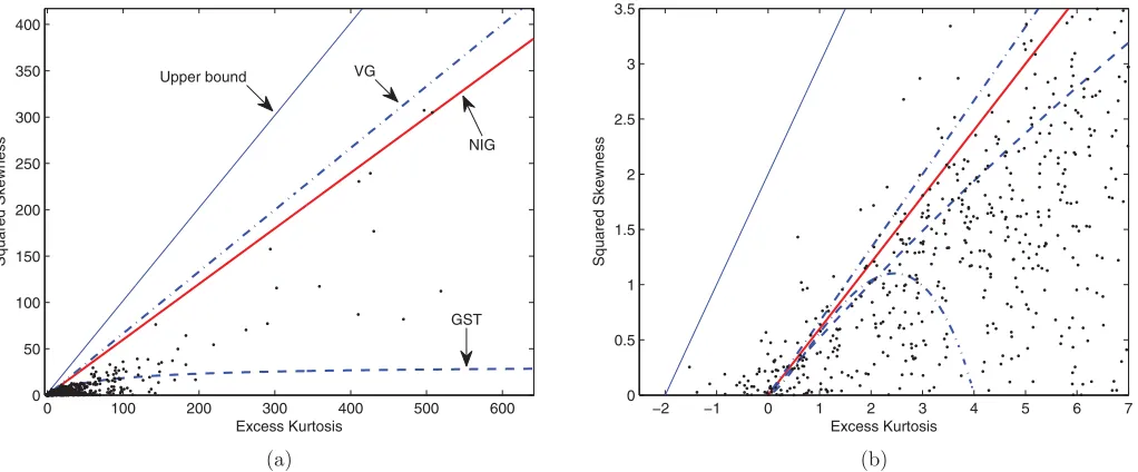
The very first question we address is whether the range of moments that are extracted from market data fall within the feasible domain of the respective densities.Figure 1plots daily skewness and kurtosis extracted from S&P 500 index options with 5–14 days to maturity for a sample covering January 4, 1996, to October 30, 2009.8There are 1258 dots inFigure 1(a).
Each dot represents a daily combination of squared skewness and excess kurtosis calculated via expressions (13) and (14). The pairs of OTM call/put options involved in the calculation of risk neutral moments per day ranges from 3 to 85, with an average of 21.26 (seeTable 1).
Superimposed on the dots are the feasible domains of the NIG, VG, and GST distributions, that is, the area under the curves with labels “VG,” “NIG,” and “GST,” respectively. The line labeled “Upper bound” represents the largest possible
7As noted by Dennis and Mayhew (2002) and Conrad, Dittmar, and Ghysels
(2013), it is critical to select a set of puts and calls that are symmetric in strike prices. In contrast, discretely weighted sums of asymmetrically positioned puts/calls result in biases.
8The data are obtained from Optionmetrics through Wharton Research Data
Services. A number of data filters are applied to screen for recording errors -these are standard in the literature and described elsewhere, see, for example, in Battalio and Schultz (2006) and Conrad, Dittmar, and Ghysels (2013), among others. Notably we use filters to try to ensure that our results are not driven by stale or misleading prices. In addition to eliminating option prices below 50 cents and performing robustness checks with additional constraints on option liquidity, we also remove options with less than one week to maturity, and eliminate days in which closing quotes on put-call pairs violate no-arbitrage restrictions. We encountered some days with two pairs of OTM call/put options. The literature often puts a lower bound of three pairs to avoid noisy moment estimates.
0 100 200 300 400 500 600 0
50 100 150 200 250 300 350 400
Excess Kurtosis
Sq
u
ared Ske
w
ness
Upper bound VG
NIG
GST
(a)
−2 −1 0 1 2 3 4 5 6 7
0 0.5 1 1.5 2 2.5 3 3.5
Excess Kurtosis
Sq
u
ared Ske
w
ness
(b)
Figure 1. Daily squared skewness and kurtosis of SPX from January 1996 to October 2009. Panel (a) plots the daily squared skewness and excess kurtosis extracted from the S&P 500 index options with 5–14 days to maturity for a sample covering January 4, 1996, to October 30, 2009. Superimposed are the feasible domains of the NIG, VG, and GST distributions, that is, the area under the curves with labels “VG,” “NIG,” and “GST,” respectively. The line labeled “Upper bound” represents the largest possible skewness-kurtosis combination of an arbitrary random variable. When zooming in on Panel (a) we obtain Panel (b). The area under the curve with a range of excess kurtosis from 0 and 4 is the feasible domain of A-type Gram-Charlier series expansion (GCSE).
skewness-kurtosis combination of an arbitrary random variable, and it is obtained by the formulaS2
=K +2. The region above the bound is the so-called impossible region. As reported in Ta-ble 1, the VG-feasible region covers 94.54% of the data points, and the NIG feasible region covers 92.59%. Finally, the cover-age of the GST feasible region is 81.44% of the data points.
Table 1 summarizes coverage of VG, NIG, and GST dis-tributions, and number of contracts used to compute the risk neutral moments. Though the VG, NIG, and GST distributions cannot accommodate any arbitrary skewness-kurtosis combina-tions, most of the S&P 500 options with short maturities feature skewness-kurtosis combinations within the feasible region of the VG and NIG distributions. The number of contracts listed inTable 1deserves some clarification. The smallest number of contracts is 3. This does not mean that we fit four moments with three prices. The header in the table says “put/call pairs.” Three prices, means 6 contracts, 3 puts, and 3 calls. This prompts the question as to how many contracts are needed to obtain reliable moment estimates. This is not so straightforward to answer, but is discussed notably in Dennis and Mayhew (2002). The
accu-racy depends not only on the number of contracts, but also how well they cover the range over which to compute the discrete approximations to the integral formulas discussed earlier.
When we zoom inFigure 1(a) we obtain the next plot (b). The area under the curve with a range of excess kurtosis from 0 and 4 is the feasible domain of A-type Gram-Charlier se-ries expansion (GCSE). The A-type GCSE and the Edgeworth expansion have been studied by Madan and Milne (1994), Ru-binstein (1998), Eriksson, Ghysels, and Wang (2009), among others as a way to approximate the unknown risk neutral den-sity. Since the Edgeworth expansion admits a smaller feasible region than the A-type GCSE (see Barton and Dennis1952for more detail), we only draw the feasible domain of the A-type GCSE inFigure 1. Clearly, most of the dots are outside the fea-sible region of the A-type GCSE and, hence, outside the feafea-sible region of the Edgeworth expansion.
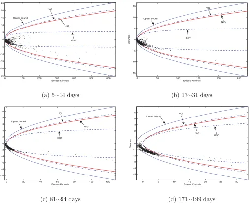
Figure 2plots the squared skewness and excess kurtosis using options with longer time to expiration: 17–31 days (around 1 month), 81–94 days (around 3 months), and 171–199 days (around 6 months).Table 1contains again the numerical values
Table 1. Coverage of VG, NIG, and GST distributions
Pairs of call/put
Total min max average VG NIG GST Impossible region
5–14 1258 3 85 21.26 94.54% 92.59% 81.44% 0
17–31 1855 3 90 22.22 74.45% 69.06% 50.08% 0
81–94 1220 3 61 13.96 23.89% 15.66% 3.63% 34/1220
171–199 1294 3 39 11.54 8.06% 5.43% 3.47% 25/1294
The table reports the number of contracts used to compute the daily risk neutral moments, and the coverage of the VG, NIG, and GST distributions for the S&P 500 index options with 5–14, 17–31, 81–94, and 171–199 days to maturity, from January 4, 1996 to October 30, 2009.
0 50 100 150 200 250 0
20 40 60
80 100 120
Excess Kurtosis
Sq
u
ared Ske
w
ness
Upper bound VG
NIG
GST
(a) TTM: 17∼31 days
−2 −1 0 1 2 3 4 5 6 7
0 0.5 1 1.5 2 2.5 3 3.5
Excess Kurtosis
Sq
u
ared Ske
w
ness
(b) TTM: 17∼31 days
0 20 40 60 80 100 120
0 5 10 15 20 25 30
Excess Kurtosis
Sq
u
ared Ske
w
ness
Upper bound VG
A−GCSE
GST
NIG
(c) TTM: 81∼94 days
0 5 10 15 20 25 30
0 2 4 6
8
10 12 14 16 18
Excess Kurtosis
Sq
u
ared Ske
w
ness
Upper bound VG
NIG
GST
A−GCSE
(d) TTM: 171∼199 days
Figure 2. Daily squared skewness and kurtosis of SPX from January 1996 to October 2009, continued.
of the feasible domain coverage for the various distributions. The VG feasible region covers 74.45% of the data points (out of 1855 contracts) for 17–31 days to maturity, and 23.89% (out of 1220) for 81–94 days to maturity. Moreover, when the time-to-maturity increases to 171–199 days, the coverage drops to 8.06% (out of 1294). These observations are consistent with the fact that the returns are more leptokurtic when sampled more frequently. It should also be noted that a few data points in Figure 2(c)–(d) are in the impossible region – 2.78% (81–94) and 1.93% (171–199), respectively, according to the figures in the last column ofTable 1. This could be due to estimation error in the moments. Moreover, we plot in Figure 3the skewness and excess kurtosis for the various time-to-maturities. This is consistent with the study of Bakshi, Kapadia, and Madan (2003) that “the risk neutral distribution of the index is generally left skewed.”
The overall picture that emerges from our analysis so far is that the classes of distributions we examine have appeal-ing properties in terms of the skewness-kurtosis coverage—in particular, when compared with approximating densities (e.g., A-type GCSE and the Edgeworth expansion) proposed in the
prior literature. The feasible domain does become more restric-tive for longer term maturities beyond 3 months. We, therefore, focus on options with maturities up to 1 month.
3.3 Simulation Evidence
We want to assess the accuracy of the various distributions via a simulation experiment. To do so we characterize risk neu-tral densities with a commonly used framework in financial asset pricing and risk management, namely continuous time jump diffusion processes. We also consider the GARCH option pricing models for the numerical evaluation. In particular, we simulate the log prices using either affine jump-diffusions or a GARCH(1,1), which yield explicit expressions for the risk neutral density and option prices. We select parameters that are empirically relevant, allowing us to assess numerically how ac-curate the various approximating distributions are in realistic settings. The discussion will focus again on the VG, NIG, and GST distributions.
3.3.1 Affine Jump-Diffusion Models. Suppose that the log price processYt=ln(St) is generated from the following affine
0 100 200 300 400 500 600
Figure 3. Daily skewness and kurtosis of SPX from January 1996 to October 2009.
jump-diffusion model under the risk neutral measure:
dYt = r−λJμ¯ −
whereNt is a compound Poisson process with L´evy measure ν(dy)=λJf(dy),and ¯μ=
Re
yf
(dy)−1 is the mean jump size.W1, W2are two independent Brownian motions, and are independent ofNtas well.
For anyu∈C,the conditional characteristic function ofYT at timetis
+aσ2 (see Duffie, Pan, and Singleton 2000). The density function of YT conditional on information up to time t is therefore ft(y;T , xt) = π1
∞
0 e−
iuy
t(iu;T , xt)du, which follows from inverse Fourier transform. The price of European call option written onY with maturityT and strike price K is defined as Ct(K;T , xt) = E((eYT −K)+|Ft), sents the imaginary part of a complex number (see Duffie, Pan, and Singleton 2000). The put price follows from the put/call parity. In the numeric calibration, we apply the fast Fourier transform of Carr and Madan (1999) to both ft(y;T , xt) and Ct(K;T , xt) (see also Lee2004). The details are in AppendixB. We focus exclusively on two cases involving jumps: Gaus-sian jumps, that is, Reuyf(dy) = exp(μJu+σJ2u
2/ 2), and exponential jumps, that is,Reuyf(dy)=(1−uμJ)−1, as they represent the most realistic processes. The model parameters are taken from Duffie, Pan, and Singleton (2000):r=3.19%,
0 100 200 300 400 500 600 700 800 900 1000
Figure 4. Skewness and kurtosis of noisy option prices generated by the AJD model. The figure displays the squared skewness and excess kurtosis calculated from the noisy option prices which are constructed by multiplying a Gamma-distributed noise to the option prices calculated from affine jump-diffusion (15) with Gaussian Jumps (see Panel (a)) and Exponential Jumps (see Panel (b)). Superimposed, we draw the feasible domains of the VG, NIG, and GST distributions.
ρ= −0.79, θ=0.014, κ=3.99, σ=0.27, λJ=0.11. We con-siderμJ = −0.14,andσJ =0.15 for Gaussian jumps, while μJ =0.14 for Exponential jumps. To determine the value of x0=(y0, v0), we simulate the log price process starting from value 0 and draw from the invariant distribution of the volatility process which is a Gamma distribution with characteristic func-tion φ(u) = (1−iuσ2/(2κ))−2θ κ/σ2
(see, e.g., Keller-Ressel 2011). We simulate 1000 sample paths. For each, we drop the first 1000 observations and use the 1001th observation from simulation as the value ofx0.
Note that in reality, the observed option prices might de-viate from the true prices due to mistakes in the recording of data, bid-ask spread, nonsynchronicity, liquidity premia, or other market frictions. We add observational errors to the simulated call/put prices. The “observed” call/put prices are constructed by multiplying a noise ǫ to the theoreti-cal theoreti-call/put prices, that is, C0∗(K;T , x0)=ǫC0(K;T , x0) and
P0∗(K;T , x0)=ǫP0(K;T , x0). The noise ǫ is assumed to be Gamma distributed with mean 1 and variance s where s is the bid-ask spread. Note that the spread is larger for the in-the-money options than for the OTM options. We set s=min(M(C0(K;T , x0)), M(C0(K;T , x0)+K−y0), which is the maximum spread allowed by the Chicago Board Options Exchange.M(·) is a piecewise linear function on the interval [0,50], with knotsM(0)=1/8,M(2)=1/4,M(5)=3/8,M(10)
=1/2,M(20)=3/4, andM(q)=1 forq ≥50.9We eliminate
option prices which violate the arbitrage-free bounds.
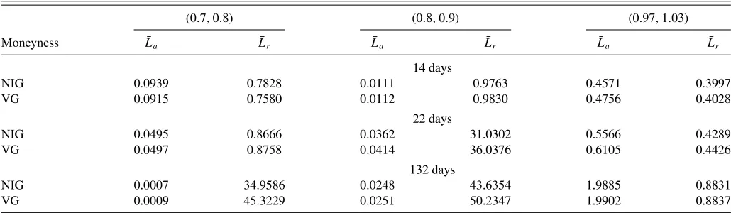
We use the approximating densities to price European call op-tions and compare them with the observed pricesC0∗(K;T , x0). Two measures of pricing errors are considered. The first is based on absolute price difference, denoted byLa. The second is de-fined in terms of relative price difference, denoted byLr. The
9See Bondarenko (2003) for more details.
two measures are defined as follows:
La =
i represent the “observed” price and the price estimated from the approximating distribution. The sum is taken over a range of strikes (or moneyness, which is the ratio of asset priceStand strike priceKi) for contracts written on the same security. These measures are, respectively, absolute and relative pricing errors.
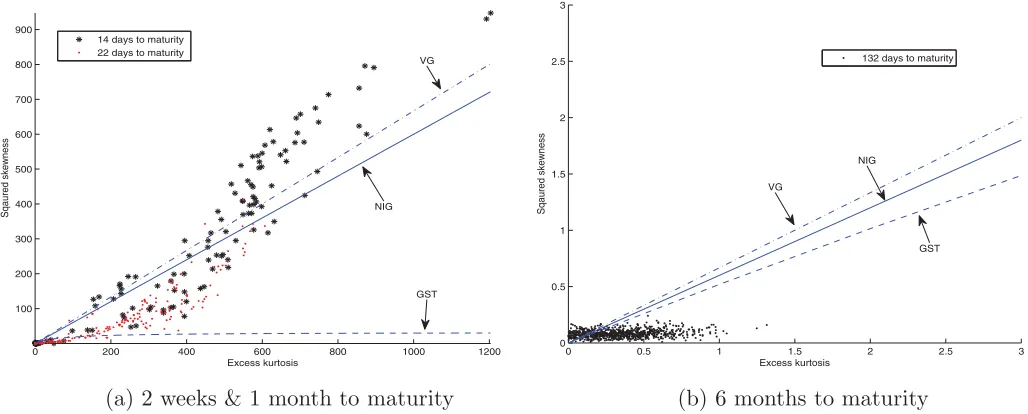
Figure 4displays the skewness and kurtosis calculated from the noisy option prices which are generated from AJD models with Gaussian jumps and Exponential jumps, respectively, for T =1/12 (in years) and 1/2 (in years).10 Table 2reports the
mean pricing errors ¯La and ¯Lr, an average ofLa andLr over 1000 iterations, for three different ranges of moneyness.Figure 4 shows that the most of the skewness-kurtosis combinations are within the feasible domain of the NIG and VG distributions, but the GST is inadequate in terms of feasible domain coverage— for both the Gaussian and Exponential jump cases. This is why we cover inTable 2 only the NIG and VG cases. The pricing errors of the two approximating densities are quite similar— particularly in absolute terms. In relative measures (using the Lr loss function) it seems that the NIG has a slight edge for short maturities (1 month) while the reverse is true for the longer maturity (6 months). Yet, in terms of feasible domain and pricing
10It is worth noting that we applied Kolmogorov-Smirnov tests to see whether
there were significant differences between the model-based densities and the approximating ones. In almost all cases we rejected the null of identical distribu-tions. The Kolmogorov-Smirnov test statistics reflect overall fit, however, while we will focus on the parts of the distributions that matter for risk management.
Table 2. Mean pricing errors for the noisy call prices generated by the AJD model
Gaussian jump Exponential jump
(0.7,0.8) (0.8,0.9) (0.97,1.03) (0.7,0.8) (0.8,0.9) (0.97,1.03)
¯
La L¯r L¯a L¯r L¯a L¯r L¯a L¯r L¯a L¯r L¯a L¯r
1 month
NIG 0.0000 1.2315 0.0000 1.5701 0.0014 0.2298 0.0001 0.2972 0.0002 0.2919 0.0019 0.2377
VG 0.0000 1.2944 0.0001 2.8800 0.0022 0.3409 0.0001 0.3096 0.0002 0.4269 0.0030 0.3091
6 months
NIG 0.0000 1.6878 0.0003 0.8600 0.0019 0.0557 0.0003 0.2501 0.0010 0.2608 0.0023 0.0668
VG 0.0000 1.5009 0.0003 0.9554 0.0021 0.0667 0.0003 0.2327 0.0014 0.3616 0.0037 0.1140
The table reports the mean pricing errors for the noisy call prices in terms of ¯Laand ¯Lr—an average of absolute pricing errorLaand relative pricing errorLrover 1000 iterations—for
three different ranges of moneyness: (0.7,0.8), (0.8,0.9), and (0.97,1.03). The noisy option prices are constructed by multiplying a Gamma-distributed noise to the option prices calculated from affine jump-diffusion (15) with Gaussian jumps and exponential jumps, respectively.
errors it is fair to say that the two classes of distributions are comparable.
3.3.2 GARCH Option Pricing Models. Besides the affine jump-diffusion models, we also consider the GARCH(1,1) op-tion pricing model of Heston and Nandi (2000)—see also Duan (1995)—to assess the approximation errors of the VG, NIG, and GST distributions. We consider the GARCH option pricing ex-ample as a reasonable alternative—used by practitioners as well as academics. Many other models—such as stochastic volatility models—require quite involved estimation procedures and fil-tering of latent volatilities. The GARCH option pricing model is arguably on the same level of simplicity as our moment-implied density approach. Many other methods are much more involved and harder to implement.
The GARCH(1,1) process under the risk neutral measure is
ln St St−1
=r−1 2σ
2
t +σtǫt, ǫt
iid
∼N(0,1)
σt2=ω+a(ǫt−1−cσt−1)2+bσt2−1. (18) The time-tprice of European call option with strikeKat maturity Tis explicitly given by
Ct
K;T , St, σt2+1
= 1
2
St−Ke−r(T−t)
+e
−r(T−t)
π
× ∞
0
Re
K−iφf(t, T;iφ+1)
iφ ]dφ
− K
∞
0
Re
K−iφf(t, T;iφ) iφ
dφ
, (19)
wheref(t;T , φ)=Stφexp(At+Btσt2+1) and
At =φr+At+1+ωBt+1−0.5 ln(1−2aBt+1)
Bt =φ(−0.5+c)−0.5c2+
0.5(φ−c)2 1−2aBt+1 +
bBt+1 (20)
with terminal conditionAT =BT =0.
The values of parameters are taken fromTable 1of Heston and Nandi (2000): r=0, ω=5.02∗10−6, a=1.32∗10−6,b= 0.589,c=422. We simulate 2000 daily prices under the risk neutral measure, with initial state variablesS0=100 andσ12= (0.152)/252. We drop the first 1000 observations, so we end up with a sample path of 1000 daily observations{(St, σt2+1), t= 1, . . . ,1000}. For eacht, we calculate the call price via (19) and put price using the put/call parity, withT =22 (in days) or 1 month and T =132 (in days) or 6 months. We also consider 14 days to maturity which is more relevant to the option pricing exercise in Section4.2. Moreover, as described in Section3.3.1, we add Gamma-distributed noise to the theoretical option prices.
Table 3. Mean pricing errors for the noisy call options simulated from the GARCH model
(0.7,0.8) (0.8,0.9) (0.97,1.03)
Moneyness L¯a L¯r L¯a L¯r L¯a L¯r
14 days
NIG 0.0939 0.7828 0.0111 0.9763 0.4571 0.3997
VG 0.0915 0.7580 0.0112 0.9830 0.4756 0.4028
22 days
NIG 0.0495 0.8666 0.0362 31.0302 0.5566 0.4289
VG 0.0497 0.8758 0.0414 36.0376 0.6105 0.4426
132 days
NIG 0.0007 34.9586 0.0248 43.6354 1.9885 0.8831
VG 0.0009 45.3229 0.0251 50.2347 1.9902 0.8837
The table reports the mean pricing errors for the noisy call prices in terms of ¯Laand ¯Lr—an average of absolute pricing errorLaand relative pricing errorLrover 1000 iterations—for
three different ranges of moneyness: (0.7,0.8), (0.8,0.9), and (0.97,1.03). The noisy option prices are constructed by multiplying a Gamma-distributed noise to the option prices calculated from (19).
0 200 400 600 800 1000 1200 100
200 300 400 500 600 700
800 900
Excess kurtosis
Sqa
u
red ske
w
ness
14 days to maturity 22 days to maturity
NIG VG
GST
(a) 2 weeks & 1 month to maturity
0 0.5 1 1.5 2 2.5 3
0 0.5 1 1.5 2 2.5 3
Excess kurtosis
Sqa
u
red ske
w
ness
132 days to maturity
VG
NIG
GST
(b) 6 months to maturity
Figure 5. Skewness and kurtosis of noisy option prices generated by the GARCH model. The figure displays the squared skewness and excess kurtosis calculated from the noisy option prices which are constructed by multiplying a Gamma-distributed noise to the option prices calculated
from the GARCH(1,1) option pricing model (18). Superimposed, we draw the feasible domains of the VG, NIG, and GST distributions.
The noisy prices, which violate the arbitrage-free bounds, are removed.
Figure 5displays the squared skewness and excess kurtosis calculated from the noisy option prices with 14 days and 22 days to maturity (Panel (a)) and 132 days to maturity (Panel (b)). Su-perimposed are the feasible domains of the VG, NIG, and GST distributions. Since the GST distribution has a more restrictive feasible domain, we consider only the VG, NIG distributions to approximate the option prices implied by the GARCH(1,1). The mean pricing errors are reported inTable 3. The VG and NIG approximations do a poor job in terms of the relative measure for the deep OTM options with time-to-maturity over 1 month. When the time-to-maturity changes from 6 months to 2 weeks, the relative pricing error decreases significantly for all the three moneyness ranges, and the two distributions—VG and NIG—are comparable.
4. OPTION PRICING
We start from the observation that a good method of option pricing should be able to price contracts in situations where only a few contracts are traded. We, therefore, design experiments where we compute risk neutral moments using a smaller set of option contracts than is available. We then price contracts which are not used to compute the moments via the approximate densities. This means we use a subset of existing market prices to extract risk neutral moments and another set of existing market prices to appraise the accuracy of the approximate option prices. Hence, we will examine, through an experimental design, how data sparseness affects option pricing via VG, NIG, and GST density approximations. We do this in such a way that we can appraise how well our methods perform to price options that are deep out-of-the-money versus options that are not. The former is the most challenging task to achieve for any method—and we show that we do very well. It will be helpful to explain the
empirical investigation first with an illustrative example—which is covered first—followed by a full sample implementation.
4.1 An Illustrative Empirical Case
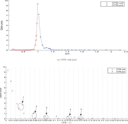
We start with an illustrative example and then proceed to a full sample formal analysis. To illustrate the design we use SPX options (European options on the S&P 500 index) priced on September 23, 2009 (which is a Wednesday) with 7 days to maturity (i.e., September 30, 2009) to illustrate the procedure. There are 42 call options and 42 put options with 7 days to maturity on 2009/9/23. The data consists of 20 OTM calls and 22 OTM puts.Figure 6(a) plots all the available OTM options. We then focus on the options with moneyness (i.e., the ratio of index levelS and strike priceK) between 0.8 and 1.2, which are displayed inFigure 6(b). Since the valuation of formulas (8), (9), and (10) require the calls and put to have the same (or similar) distance from strike price to the index level to mitigate estimation error (recall the discussion in footnote 7), we use
|K/S−1|asx-axis inFigure 6(b). To evaluate the option pricing via the VG, NIG, and GST approximations and assess how data sparseness affects pricing accuracy, we consider two strategies: (1) select the call/put pairs with|K/S−1|closest to 0.03, 0.06, 0.09, 0.12, and 0.15, and (2) select the call/put pairs with|K/S− 1| closest to 0.03, 0.09, and 0.15. Therefore, we pick call/put pairs in Circles 1–5 inFigure 6(b) for Strategy 1, and call/put pairs in Circles 1, 3, and 5 for Strategy 2. For each strategy, we derive the approximating densities—the VG, NIG, and GST distributions, and then price all the “unused” call options.11
Table 4 reports the pricing errors measured byLa andLr (defined in (17) whereCiobsis the observed market call option price). Denote by [a, b] the range of moneyness of call options
11We do not consider call options with moneyness greater than 1.03, because
they are not liquid, that is, infrequently traded.
0.8 1 1.2 1.4 1.6 1.8 2 2.2 0
1 2 3 4 5 6 7 8 9 10
S/K
Option price
OTM call
OTM put
(a) OTM calls/puts
0 0.01 0.02 0.03 0.04 0.05 0.06 0.07 0.080.09 0.1 0.11 0.12 0.13 0.14 0.15 0.16 0.17 0.180.19 0.2 0.21 0.22 0.23 0.24 0.25 0
1 2 3 4 5 6 7 8 9 10
| K/S − 1 |
Option price
OTM call OTM put
3 2
1
4 5
(b) Data used
Figure 6. OTM SPX calls and puts, 2009/9/23, expired on 2009/9/30. The figure plots all the available out-of-the-money S&P 500 index call/put options priced on September 23, 2009 with 7 days to maturity.
that are used for pricing. We divide all the “unused” calls into three groups: Group 1 contains “unused” options with mon-eyness within [a, b], Group 2 contains “unused” options with moneyness less thana, and Group 3 contains “unused” calls with moneyness greater thanb. In particular:
• Strategy 1:a=0.8660 andb=0.9733. There are 2 points in [a, b], 10 points in ‘< a’, 4 points in ‘> b’, a total of 16 unused points.
• Strategy 2:a=0.8660 andb=0.9733. There are 4 points in [a, b], 10 points in ‘< a’, 4 points in ‘> b’, a total of 18 unused points.
The three groups are labeled as [a, b],< a, and> b, respec-tively, inTable 4. The following observations emerge from ex-aminingTable 4:
• The GST approximation is not feasible using Strategy 1, while it is for Strategy 2.
Table 4. Pricing SPX call options on 2009/9/23
Overall [a, b] < a > b
La Lr La Lr La Lr La Lr
Strategy 1
NIG 2.6837 0.9449 0.6992 0.9606 0.0675 0.9998 5.3434 0.7816
VG 3.1201 0.9194 0.6105 0.7757 0.0674 0.9893 6.2244 0.7962
GST NA NA NA NA NA NA NA NA
Strategy 2
NIG 2.2326 0.8451 0.3739 0.6122 0.0673 0.9782 4.7200 0.6685
VG 2.4797 0.8147 0.3193 0.4496 0.0672 0.9597 5.2494 0.6942
GST 2.0950 0.9493 0.5315 1.0000 0.0675 1.0000 4.4110 0.7454
The table reports the pricing errors measured byLaandLr(defined in (17) whereCobsi is the observed market call option price) for S&P 500 index call options on September 23, 2009,
with 7 days to maturity. Two strategies are considered. For Strategy 1, we use five pairs of call/put options to construct the approximating VG, NIG, and GST distributions, which are further used to price other unused options. For Strategy two, three pairs of call/put options are selected to do the pricing. Denote by [a, b] the range of moneyness of call options that are used for pricing. We divide all the “unused” calls into three groups: Group 1 contains “unused” options with moneyness within [a, b], Group 2 contains “unused” options with moneyness less thana, and Group 3 contains “unused” calls with moneyness greater thanb. The three groups are labeled as [a, b],< a, and> b, respectively.
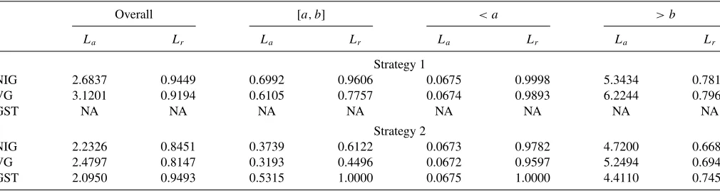
• The pricing errors are relatively small in Strategy 2. In other words, the accuracy is improved when we use fewer options to derive the NIG, VG, and GST approximations.
• Overall, the VG approximation is best, though Strategy 1 picks NIG and Strategy 2 picks GST for group 3—perhaps in light of a small sample size in that group.
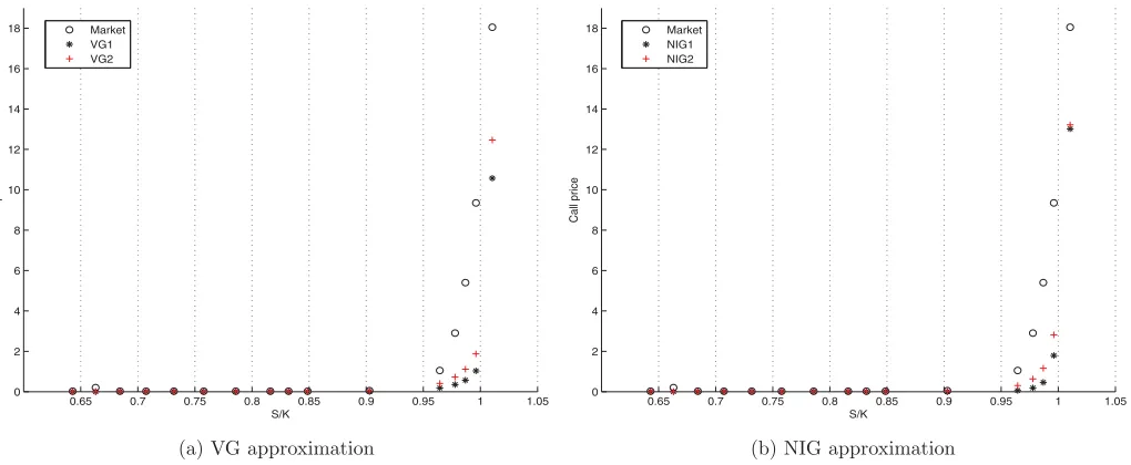
Since Strategy 2 yields a smaller pricing error than Strategy 1 in terms of both absolute and relative measures, we take a closer look at this phenomenon. There are 16 “unused” calls in Strategy 1 and 18 in Strategy 2. We pick up the “unused” call options in common (i.e., 16) and compare their market values with the prices derived from both strategies. The results are shown inFigure 7, where “VG1” and “NIG1” refer to the option prices estimated by VG and NIG, respectively, using Strategy 1, while “VG2” and “NIG2” are for Strategy 2. “Market” means the observed market price. It is apparent that the prices derived from Strategy 2 is much closer to the market prices, especially for the at-the-money (ATM) options (i.e., S/K between 0.97 and 1.03).
Since the pricing errors are smaller in Strategy 2 with fewer observations, we have that the accuracy is improved when fewer options are used to derive the NIG, VG, and GST approxima-tions. This may sound counterintuitive since usually more ob-servations often lead to high accuracy. It is worth recalling that we are dealing with approximate models where more data may either improve or worsen the approximation. Hence, we are not in a regular setting of sampling theory with increased accuracy with more data. This explains why fewer observations may, as it turns out, be better.
4.2 Full Sample Analysis
We examine now all the SPX options from January 4, 1996 to October 30, 2009, which are priced on Wednesdays.12 For
each Wednesday and time-to-maturityT0, we pick the ATM call
12We pick Wednesday—as this is common in the empirical option pricing
literature—since it avoids some of the day-of-the-week effects that occur par-ticularly on Fridays and Mondays.
option with strike price closest to the index level, and then cal-culate its Black-Scholes implied volatility (IV). We, therefore, obtain a sample of IVs for time-to-maturityT0. Based on this sample, we obtain the empirical first and third quartiles, that is, Q1andQ3. Denote byD(1, T0) all the Wednesday calls whose IV is less thanQ1,D(2, T0) the Wednesday calls whose IV is betweenQ1 andQ3, andD(3, T0) the set of Wednesday calls whose IV is larger thanQ3. Based on observations in Section
3.2, we considerT0as one week (i.e., 5–14 days), 1 month (i.e., 17–31 days), and 3 months (i.e., 81–94 days). Therefore, we end up with nine different combinations.Table 5lists, for each combination, the number of days which yield skewness-kurtosis combination within the feasible domain of the VG, NIG, GST distributions using Strategies 1 and 2, respectively.13Namely, the triplets inTable 5are the numbers of days feasible for the VG, NIG, and GST distributions. For instance, the triplet (27,21,0) means that the VG distribution can model 27 dates out of 46 (i.e., first quartile yields 46 data points), NIG can model 21 data points while none of the 46 days yields a skewness-kurtosis combination in the feasible domain of the GST distribution. We note that, as expected, the GST is the most restrictive. We, therefore, consider two sample configurations—one where all three distributions are applicable. This is a relatively small sam-ple that arguably gives unfair advantage to the more restrictive GST distribution. Hence, we also examine a sample where only the VG and NIG distributions are feasible. This is a larger and hence more reliable sample. We analyze the pricing errors for days identified inTable 5starting with the most restrictive sam-ple configurations involving all days where GST, VG, and NIG distributions apply. We focus on the setD(2, T0) withT0=17– 31 and 81–94,D(3, T0) withT0=5–14 and 17–31 because they have relatively more observations than the other cells. For days identified in each of the cells, we repeat the analysis described for the single day 2009/9/23, and deriveLa andLr.We then averageLaandLrwithin each cell. These averages, denoted by
¯
Laand ¯Lrrespectively, are reported inTable 9.
To appraise the performance of the VG, NIG, and GST approximations, we use the prices computed from the
13We removed days which have fewer than five calls or five puts.
0.65 0.7 0.75 0.8 0.85 0.9 0.95 1 1.05 0
2 4 6
8
10 12 14 16 18
S/K
Call price
Market VG1 VG2
(a) VG approximation
0.65 0.7 0.75 0.8 0.85 0.9 0.95 1 1.05 0
2 4 6
8
10 12 14 16 18
S/K
Call price
Market
NIG1
NIG2
(b) NIG approximation
Figure 7. Compare Strategy 1 with Strategy 2 for SPX call options on September 23, 2009. The figure compares the market prices of 16 call options (on September 23, 2009 with 7 days to maturity) with the prices derived from Strategy 1 and Strategy 2. “VG1” and “NIG1” refer to the option prices estimated by VG and NIG, respectively, using Strategy 1, while “VG2” and “NIG2” are for Strategy 2. “Market” means the observed market price.
Black-Scholes model and the GARCH(1,1) option pricing model (18) as benchmarks, which will be denoted BLS and GARCH, respectively, in the tables. The volatility that enters the Black-Scholes formula is the Black-Scholes implied volatil-ity of the previous-day ATM call option, which has the shortest time-to-maturity and strike price closest to the index level.14To
obtain the GARCH option pricing (19), we first estimate model parameters by considering the following GARCH(1,1) under the physical measure
ln St St−1
=r+λσ˜ t2+σtǫt, ǫt ∼N(0,1)
σt2=ω+a(ǫt−1−cσ˜ t−1)2+bσt2−1. (21)
We use the S&P 500 index over the full sample—from January 4, 1996 to October 30, 2009 to estimate the pa-rameters (a, b,c, ω,˜ λ˜). The maximum likelihood estima-tors are ( ˆa,b,ˆ c,ˆ˜ ω,ˆ λˆ˜) = (1.72e−05,0.4895,164.1,7.5e− 05,1.4685), and hence ˆc=cˆ˜+λˆ˜ +.5=166.0685.
What do we learn fromTable 9? For median volatility regimes (D(2, .)) we note that option pricing based on Black-Scholes implieds perform best in absolute terms (La) but not in relative terms. This observation applies to both strategies and across moneyness. In terms of relative pricing errors the picture is quite different. Namely, in terms of relative pricing errors, we find that either the VG approximation or the GST one is the best. It should also be noted, however, that the NIG and VG approximations typically yield similar relative pricing errors. The GST appears to perform better for ATM options> b.It is also worth noting that Strategies 1 and 2 yield comparable pricing errors. This is rather impressive as it means that we can use less data (i.e., contracts) and still find similar pricing errors.
14This is considered the most heavily traded and accurately priced contract; see
Bates (1995) and Chernov and Ghysels (2000).
In turbulent times (D(3, .)) we note that BLS starts to per-form poorly both in absolute and relative pricing error terms. Overall—all maturities pooled—we find GST to perform best in absolute terms, but the VG approximation is again clearly dominant, with NIG quite similar in terms of performance. It is clear that the distributional approximations make a big dif-ference compared to Black-Scholes implied option pricing as the pricing errors are substantially larger for BLS. In terms of relative pricing errors, the differences between BLS and distri-butional approximations are particularly important.
What happens when we drop the GST distribution, which is most restrictive in terms of feasibility? The results—where we remove the GST distribution—appear in Table 10. Given the different sample configuration, we look at a larger set of combinations, namely, we look at the sets D(1, T0) with T0
=5–14 and 17–31,D(2, T0) withT0 =5–14, 17–31 and 81– 94, and finally D(3, T0) with T0 =5–14 and 17–31. Hence, we not only looking at a larger dataset within each cell (see Table 5) but also a broader set of maturity/moneyness/volatility-state combinations. We start with the cases that are common
Table 5. Number of days that yield skewness-kurtosis combination within the feasible domains of the VG, NIG, GST distributions, SPX
options (1996–2009)
T0 Total Strategy D(1, T0) D(2, T0) D(3, T0)
5∼14 184 1 (27, 21, 0) (66, 55, 3) (41, 39, 19)
2 (34, 28, 2) (78, 76, 32) (43, 40, 32)
17∼31 352 1 (34, 22, 1) (114, 88, 15) (60, 48, 25)
2 (65, 55, 2) (142, 126, 40) (62, 53, 31)
81∼94 255 1 (16, 7, 0) (52, 36, 17) (5, 4, 4)
2 (22, 10, 0) (43, 30, 14) (4, 4, 3)
The table lists, for each of nine combinations, the number of days which yield the risk neutral skewness-kurtosis combination within the feasible domains of the VG, NIG, GST distributions using Strategies 1 and 2, respectively. The skewness and kurtosis are extracted from S&P 500 index options from January 4, 1996 to October 30, 2009.
between Tables9 and10. We note that whenever GST is best when feasible the NIG distribution fills the void. However, since NIG and VG are again often close—it is also the case that VG is equally appealing. Overall, we find quantitatively the same results as in the more constraint sample where GST is feasible. Namely, Strategies 1 and 2 appear similar, the absolute pricing errors are dominated by BLS in the low volatility regime—as before—but in terms of relative pricing errors there are clear gains across all moneynesses and maturities. Moreover, once we move to high volatility states BLS no longer performs well. Finally, it is also worth noting that the GARCH option pricing model reported in Tables9and10performs very poorly, both in absolute and relative terms. Hence, the methods we propose are clearly superior to the GARCH option pricing model.
5. FROM THE RISK NEUTRAL MEASURE TO THE PHYSICAL MEASURE
In this section, we discuss the relation between the risk neutral measure and the physical measure in terms of the first four moments.
Letft(x;τ) be the conditional density function ofRt(τ)= ln(St+τ)−ln(St) at time t under the risk neutral measure Q, while ˜ft(x;τ) the conditional density under the physical mea-sure P. Consider a power utility function with coefficient of relative risk aversionθ1, and scaling factorθ0. The pricing ker-nel is then
mt(Rt(τ), θ)=θ0e−θ1Rt(τ). (22)
The physical density, risk neutral density, and utility function are related in the following way:
˜ lowing proposition links the cumulants under the risk neutral measure and the physical measure.
Proposition 5.1. Suppose that there exist 0< rq, rp < ∞ such that eyλf
t(y;τ)dy <∞ for |λ|< rq and
eyλf˜
t(y;τ)dy <∞for|λ|< rp. Letκnbe thenth cumulant ofRt(τ) conditional on information up to timetunder the risk neutral measure, and ˜κk under the physical measure. Then for l≥1,
The proof can be found in Rompolis and Tzavalis (2010). To a leading order, we have ˜κl≈κl+θ1κl+1. Moreover,κl=κ˜l− Kapadia, and Madan (2003) obtained similar results for the central moments of return.
15See A¨ıt-Sahalia and Lo (2000b), Jackwerth (2000), Rosenberg and Engle
(2002), Liu et al. (2007), among others.
LetMean( t, τ)var( t, τ),Skew( t, τ),andEKurt(t, τ) be the timet conditional mean, variance, skewness, and excess kur-tosis of ln(St+τ) under the physical measure. It follows from Proposition 5.1 that,
whereκ5needs the pricing ofE
Q Equations (25)–(28) allow us to calculate the first four moments under the physical measure.
Because the transformation formulas (25)–(28) are derived under the assumption that ˜κl≈κl+θ1κl+1, we report inTable
6 the sample mean and standard deviation of the risk neutral cumulantsκ2,κ3,κ4, andκ5for the S&P 500 index over the full sample—from January 4, 1996, through October 30, 2009.16 On average, the higher-order cumulants are of order 10−4 for time-to-maturity up to 1 month. Therefore, it is reasonable to believe that the transformation formulas (25)–(28) provide a good approximation ifθ1is relatively small, say, less than 10.
Next we will discuss in detail the VG, NIG, and GST distri-butions under the physical measure, and the estimation of the relative risk aversion coefficientθ1.
5.1 The GH Family of Distributions: The Risk Neutral Measure or the Physical Measure?
Suppose that the conditional distribution ofRt(τ) given in-formation up to timetis approximated by GH(αt, βt, μt, bt, pt) under the physical measureP. Consider the moment-generating function of GH(α, β, μ, b, p). For|β+z|< α,
16The results are similar in magnitude to the estimates ofκ
3andκ4reported
in Rompolis and Tzavalis (2010) who looked at S&P 500 index returns and options over 22 trading days from January 1996, to December 2007.
Table 6. Summary statistics for SPX from January 1996 to October 2009
Skewness Excess kurtosis κ2 κ3 κ4 κ5
5∼14 days to maturity
Mean –1.5131 22.8377 0.0015 –0.0002 0.0001 –0.0001
SD 1.7441 50.4268 0.0020 0.0005 0.0005 0.0008
17∼31 days to maturity
Mean –1.3942 7.3299 0.0037 –0.0006 0.0003 –0.0003
SD 0.8565 13.2251 0.0050 0.0018 0.0014 0.0016
81∼94 days to maturity
Mean –1.2633 3.0027 0.0129 –0.0031 0.0016 –0.0011
SD 0.6652 8.9794 0.0144 0.0076 0.0065 0.0070
171∼199 days to maturity
Mean –1.1723 1.5461 0.0258 –0.0069 0.0027 –0.0009
SD 0.5268 3.6149 0.0239 0.0138 0.0103 0.0076
The table reports the sample mean (mean) and standard deviation (SD) of the risk neutral skewness, the risk neutral excess kurtosis, and the risk neutral cumulantsκ2,κ3,κ4, andκ5for S&P 500 index over the full sample (January 4, 1996 – October 30, 2009). The risk neutral moments and cumulants are extracted from option prices via (8), (9), and (10).
wherefGH(x) is defined in (1). The pricing kernel (22) satisfies the following arbitrage free conditions
EtP[mt(Rt(τ), θt)]=e−rτ, EPt
mt(Rt(τ), θt)eRt(τ)
=1 (30)
if and only if
MGH(−θ1;αt, βt, μt, bt, pt)=θ0−1e−
rτ,
MGH(1−θ1;αt, βt, μt, bt, pt)=θ0−1 (31)
given that |βt−θ1|< αt and|βt+1−θ1|< αt.17 It follows that logMGH(1;αt, βt−θ1, μt, bt, pt)=rτ. Therefore,Rt(τ) is GH(αt, βt−θ1, μt, bt, pt) under the risk neutral measure. On the other hand, if the conditional distribution ofRt(τ) belongs to the GH family under the risk neutral measure, then after exponential tilting the real-world distribution ofRt(τ) is within the GH family as well again in the absence of arbitrage. In particular, under the arbitrage free assumption,Rt(τ) is NIG (or VG) distributed under the risk neutral measure if and only if it is NIG (or VG) distributed under the physical measure, but it does not apply to the GST distribution.
Next we will consider estimatingθ1when the approximating densities are the VG and NIG. We use the maximum likelihood estimation outlined in Liu et al. (2007). Let{t∗
i,1≤i≤n}be the expiration times of the options and lettibe the time when risk neutral densities are formed for options that expire at timet∗
i. {t∗
i, ti}should satisfyti < ti∗≤ti+1for 1≤i≤n−1 withtn∗ = tn+1so that the densities do not overlap. Withτ =ti∗−ti,θ1is estimated by maximizing the following log-likelihood function
logL(Rt1(τ), . . . , Rtn(τ)|θ1)=
n
i=1
log ˜fti(Rti(τ)|θ1,ˆti),
(32)
where ˜fti(Rti(τ)|θ1,ˆti) is the real-world distribution ofRti(τ)
conditional on information up to ti, and ˆti represents the
17See, for instance, Singleton (2006) and Le´on, Menc´ıa, and Sentana (2009).
vector of estimated parameters in the associated risk neu-tral density. To be specific, if Rti(τ) is NIG(αti, βti, μti, bti)
distributed under the risk neutral measure, then f˜ti(·) is
the density function of NIG(αti, βti +θ1, μti, bti) with ti =
(αti, βti, μti, bti). ˆti is obtained by matching the moments as
described in Section 3.1. Similarly, if Rti(τ) is modeled by
VG(αti, βti, μti, pti) under the risk neutral measure, then it is
VG(αti, βti +θ1, μti, pti) distributed under the physical
mea-sure withti =(αti, βti, μti, pti).Table 7reports the estimates
ofθ1using the S&P 500 index options from January 4, 1996, to October 30, 2009, withτ =7,14,22 days.
5.2 Value-at-Risk Forecasting
Last but certainly not least, we consider value-at-risk (VaR) forecasting. We use the notation introduced in Section 3.1.
−Rt(τ) can be viewed as the loss from time t tot+τ. The τ−period-ahead VaR forecast at level 100(1−α)% is defined as VaRt(τ, α)=infy{y:P(−Rt(τ)≥y|Ft)≤α}. We consider VaR evaluated under the risk neutral measureQas well as the physical measureP, which will be denoted by VaRQt (τ, α) and VaRPt (τ, α), respectively. LetVaR
Q
t (τ, α) (orVaR P
t (τ, α)) be the estimate of VaRQt (τ, α) (or VaRPt(τ, α)). The real-world es-timates are obtained usingθ1reported inTable 7. Therefore, only the VG and NIG distributions are considered in this exercise.
Table 7. The estimates ofθ1using SPX options from January 1996 to
October 2009
Time to maturity VG NIG
7 days 2.8953 3.0914
14 days 0.7484 0.2421
22 days 0.0140 0.0198
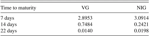
The table reports the estimates of the relative risk aversion coefficientθ1using S&P 500 index options from January 4, 1996, to October 30, 2009, with 7 days, 14 days, 22 days to maturity.
1996 1997 19981999 2000 20012002 2003 20042005 2006 2007 2008 2009 −0.15
−0.1 −0.05 0 0.05 0.1 0.15 0.2 0.25
Physical measure Risk neutral measure Loss
(a) VG approximation
1996 1997 19981999 2000 20012002 2003 20042005 2006 2007 2008 2009 −0.15
−0.1 −0.05 0 0.05 0.1 0.15 0.2 0.25
Physical measure Risk neutral measure Loss
(b) NIG approximation
Figure 8. The 95% VaR forecast for SPX over 7 days. The figure plots the losses{−Rt(7)}(the curves) of S&P 500 index from January 1996 to October 2009, and the 95% VaR forecasts under the risk neutral measure (i.e., stars forVaRQt (7,0.05)) and the physical measure (i.e., dots for
VaRPt (7,0.05)). The forecasts are derived using the VG and the NIG densities. The real world forecasts are obtained usingθ1reported inTable 7. The vertical line divides the series into two subperiods: (1) prior to August 2008 and (2) the financial crisis period.
1996 1997 1998 1999 2000 2001 2002 2003 2004 2005 2006 2007 2008 2009 −0.15
−0.1 −0.05 0 0.05 0.1 0.15 0.2 0.25 0.3
Physical measure Risk neutral measure Loss
(a) VG approximation
1996 1997 1998 1999 2000 2001 2002 2003 2004 2005 2006 2007 2008 2009 −0.15
−0.1 −0.05 0 0.05 0.1 0.15 0.2 0.25
Physical measure Risk neutral measure Loss
(b) NIG approximation
Figure 9. The 95% VaR forecast for SPX over 14 days. The figure plots the losses{−Rt(14)}(the curves) of S&P 500 index from January 1996 to October 2009, and the 95% VaR forecasts under the risk neutral measure (i.e., stars forVaRQt (14,0.05)) and the physical measure (i.e., dots forVaRPt (14,0.05)). The forecasts are derived using the VG and the NIG densities. The real world forecasts are obtained usingθ1reported inTable 7. The vertical line divides the series into two subperiods: (1) prior to August 2008 and (2) the financial crisis period.
We consider again the SPX options from January 4, 1996 to October 30, 2009, with 7 days and 14 days to maturity. Hence, we do as if we hold the market portfolio or something similar to that, and compute its VaR forecast. Figures8and9plot the losses
{−Rt(τ)}over the life time of options, that is,τ=7 and 14. The vertical line divides the series into two subperiods: (1) Prior to August 2008 and (2) the Financial crisis period.18Superimposed
are the out-of-sample VaR forecasts at the 95% level under the risk neutral measure (stars) and the physical measure (dots). The estimates are derived using the VG and the NIG densities. There are 229 observations forτ =7. Among them, 216 observations
18We also remove days which have only two pairs of contracts.
can be modeled by the VG density while 213 by the NIG density. Forτ =14, 155 out of 172 can be approximated by the VG and 149 out of 172 by the NIG density.
To better understand the difference between the VG and NIG densities and their goodness of fit, we consider the VaR fail-ure indicator which is defined asIt(τ, α)=I{−R
t(τ)>VaR P t(τ,α)},
that is,It(τ, α)=1 if Rt(τ)<−VaR P
t (τ, α) and 0 otherwise. Figure 10plots the 95% VaR forecasts under the physical mea-sure (i.e., VaRPt(τ,0.05)) using both VG and NIG densities against the losses {−Rt(τ)}over the lift time of the options forτ =7 and 14. Denote byT the number of VaR forecasts. ThenTt=1It(τ, α) is the total number of exceedances of the 100(1−α)% VaR forecasts, andT−1T
t=1It(τ, α) is referred