THE PHYSICS OF VIBRATIONS
AND WAVES
Sixth Edition
H. J. Pain
Formerly of Department of Physics,
Copyright#2005 John Wiley & Sons Ltd, The Atrium, Southern Gate, Chichester, West Sussex PO19 8SQ, England
Telephone (+44) 1243 779777
Email (for orders and customer service enquiries): [email protected] Visit our Home Page on www.wileyeurope.com or www.wiley.com
All Rights Reserved. No part of this publication may be reproduced, stored in a retrieval system or transmitted in any form or by any means, electronic, mechanical, photocopying, recording, scanning or otherwise, except under the terms of the Copyright, Designs and Patents Act 1988 or under the terms of a licence issued by the Copyright Licensing Agency Ltd, 90 Tottenham Court Road, London W1T 4LP, UK, without the permission in writing of the Publisher. Requests to the Publisher should be addressed to the Permissions Department, John Wiley & Sons Ltd, The Atrium, Southern Gate, Chichester, West Sussex PO19 8SQ, England, or emailed to [email protected], or faxed to (+44) 1243 770620.
This publication is designed to provide accurate and authoritative information in regard to the subject matter covered. It is sold on the understanding that the Publisher is not engaged in rendering professional services. If professional advice or other expert assistance is required, the services of a competent professional should be sought.
Other Wiley Editorial Offices
John Wiley & Sons Inc., 111 River Street, Hoboken, NJ 07030, USA Jossey-Bass, 989 Market Street, San Francisco, CA 94103-1741, USA Wiley-VCH Verlag GmbH, Boschstr. 12, D-69469 Weinheim, Germany
John Wiley & Sons Australia Ltd, 33 Park Road, Milton, Queensland 4064, Australia
John Wiley & Sons (Asia) Pte Ltd, 2 Clementi Loop # 02-01, Jin Xing Distripark, Singapore 129809 John Wiley & Sons Canada Ltd, 22 Worcester Road, Etobicoke, Ontario, Canada M9W 1L1
Wiley also publishes its books in a variety of electronic formats. Some content that appears in print may not be available in electronic books.
Library of Congress Cataloging-in-Publication Data (to follow)
British Library Cataloguing in Publication Data
A catalogue record for this book is available from the British Library
ISBN 0 470 01295 1 hardback ISBN 0 470 01296 X paperback
Contents
Introduction to First Edition . . . xi
Introduction to Second Edition . . . xii
Introduction to Third Edition . . . xiii
Introduction to Fourth Edition . . . xiv
Introduction to Fifth Edition . . . xv
Introduction to Sixth Edition . . . xvi
1 Simple Harmonic Motion 1
Displacement in Simple Harmonic Motion 4
Velocity and Acceleration in Simple Harmonic Motion 6
Energy of a Simple Harmonic Oscillator 8
Simple Harmonic Oscillations in an Electrical System 10 Superposition of Two Simple Harmonic Vibrations in One Dimension 12 Superposition of Two Perpendicular Simple Harmonic Vibrations 15
Polarization 17
Superposition of a Large Numbernof Simple Harmonic Vibrations of
Equal Amplitudeaand Equal Successive Phase Differenced 20 Superposition ofnEqual SHM Vectors of Lengthawith Random Phase 22
Some Useful Mathematics 25
2 Damped Simple Harmonic Motion 37
Methods of Describing the Damping of an Oscillator 43
3 The Forced Oscillator 53
The Operation of i upon a Vector 53
Vector form of Ohm’s Law 54
The Impedance of a Mechanical Circuit 56
Behaviour of a Forced Oscillator 57
Behaviour of Velocityvvin Magnitude and Phase versus Driving Force Frequencyx 60 Behaviour of Displacement versus Driving Force Frequencyx 62
Problem on Vibration Insulation 64
Significance of the Two Components of the Displacement Curve 66 Power Supplied to Oscillator by the Driving Force 68 Variation ofPavwithx. Absorption Resonance Curve 69
TheQ-Value in Terms of the Resonance Absorption Bandwidth 70
TheQ-Value as an Amplification Factor 71
The Effect of the Transient Term 74
4 Coupled Oscillations 79
Stiffness (or Capacitance) Coupled Oscillators 79
Normal Coordinates, Degrees of Freedom and Normal Modes of Vibration 81 The General Method for Finding Normal Mode Frequencies, Matrices,
Eigenvectors and Eigenvalues 86
Mass or Inductance Coupling 87
Coupled Oscillations of a Loaded String 90
The Wave Equation 95
5 Transverse Wave Motion 107
Partial Differentiation 107
Waves 108
Velocities in Wave Motion 109
The Wave Equation 110
Solution of the Wave Equation 112
Characteristic Impedance of a String (the string as a forced oscillator) 115 Reflection and Transmission of Waves on a String at a Boundary 117
Reflection and Transmission of Energy 120
The Reflected and Transmitted Intensity Coefficients 120
The Matching of Impedances 121
Standing Waves on a String of Fixed Length 124
Energy of a Vibrating String 126
Energy in Each Normal Mode of a Vibrating String 127
Standing Wave Ratio 128
Wave Groups and Group Velocity 128
Wave Group of Many Components. The Bandwidth Theorem 132
Transverse Waves in a Periodic Structure 135
Linear Array of Two Kinds of Atoms in an Ionic Crystal 138 Absorption of Infrared Radiation by Ionic Crystals 140
Doppler Effect 141
6 Longitudinal Waves 151
Sound Waves in Gases 151
Energy Distribution in Sound Waves 155
Intensity of Sound Waves 157
Longitudinal Waves in a Solid 159
Application to Earthquakes 161
Longitudinal Waves in a Periodic Structure 162
Reflection and Transmission of Sound Waves at Boundaries 163
Reflection and Transmission of Sound Intensity 164
7 Waves on Transmission Lines 171
Ideal or Lossless Transmission Line 173
Coaxial Cables 174
Characteristic Impedance of a Transmission Line 175 Reflections from the End of a Transmission Line 177
Short Circuited Transmission LineðZL¼0Þ 178
The Transmission Line as a Filter 179
Effect of Resistance in a Transmission Line 183
Characteristic Impedance of a Transmission Line with Resistance 186 The Diffusion Equation and Energy Absorption in Waves 187
Wave Equation with Diffusion Effects 190
Appendix 191
8 Electromagnetic Waves 199
Maxwell’s Equations 199
Electromagnetic Waves in a Medium having Finite Permeabilityland
Permittivityebut with Conductivityr¼0 202
The Wave Equation for Electromagnetic Waves 204
Illustration of Poynting Vector 206
Impedance of a Dielectric to Electromagnetic Waves 207 Electromagnetic Waves in a Medium of Propertiesl,eandr(wherer6¼0) 208
Skin Depth 211
Electromagnetic Wave Velocity in a Conductor and Anomalous Dispersion 211
When is a Medium a Conductor or a Dielectric? 212
Why will an Electromagnetic Wave not Propagate into a Conductor? 214 Impedance of a Conducting Medium to Electromagnetic Waves 215 Reflection and Transmission of Electromagnetic Waves at a Boundary 217
Reflection from a Conductor (Normal Incidence) 222
Electromagnetic Waves in a Plasma 223
Electromagnetic Waves in the Ionosphere 227
9 Waves in More than One Dimension 239
Plane Wave Representation in Two and Three Dimensions 239
Wave Equation in Two Dimensions 240
Wave Guides 242 Normal Modes and the Method of Separation of Variables 245
Two-Dimensional Case 246
Three-Dimensional Case 247
Normal Modes in Two Dimensions on a Rectangular Membrane 247
Normal Modes in Three Dimensions 250
Frequency Distribution of Energy Radiated from a Hot Body. Planck’s Law 251
Debye Theory of Specific Heats 253
Reflection and Transmission of a Three-Dimensional Wave at a
Plane Boundary 254
Total Internal Reflection and Evanescent Waves 256
10 Fourier Methods 267
Fourier Series 267
Application of Fourier Sine Series to a Triangular Function 274 Application to the Energy in the Normal Modes of a Vibrating String 275 Fourier Series Analysis of a Rectangular Velocity Pulse on a String 278
The Spectrum of a Fourier Series 281
Fourier Integral 283
Fourier Transforms 285
Examples of Fourier Transforms 286
The Slit Function 286
The Fourier Transform Applied to Optical Diffraction from a Single Slit 287
The Gaussian Curve 289
The Dirac Delta Function, its Sifting Property and its Fourier Transform 292
Convolution 292
The Convolution Theorem 297
11 Waves in Optical Systems 305
Light. Waves or Rays? 305
Fermat’s Principle 307
The Laws of Reflection 307
The Law of Refraction 309
Rays and Wavefronts 310
Ray Optics and Optical Systems 313
Power of a Spherical Surface 314
Magnification by the Spherical Surface 316
Power of Two Optically Refracting Surfaces 317
Power of a Thin Lens in Air (Figure 11.12) 318
Principal Planes and Newton’s Equation 320
Optical Helmholtz Equation for a Conjugate Plane at Infinity 321 The Deviation Method for (a) Two Lenses and (b) a Thick Lens 322
The Matrix Method 325
12 Interference and Diffraction 333
Interference 333
Division of Amplitude 334
Newton’s Rings 337
Michelson’s Spectral Interferometer 338
The Structure of Spectral Lines 340
Fabry -- Perot Interferometer 341
Resolving Power of the Fabry -- Perot Interferometer 343
Division of Wavefront 355
Interference from Two Equal Sources of Separationf 357 Interference from Linear Array ofNEqual Sources 363
Diffraction 366
Scale of the Intensity Distribution 369
Intensity Distribution for Interference with Diffraction fromNIdentical Slits 370 Fraunhofer Diffraction for Two Equal SlitsðN¼2Þ 372
Transmission Diffraction Grating (NLarge) 373
Resolving Power of Diffraction Grating 374
Resolving Power in Terms of the Bandwidth Theorem 376 Fraunhofer Diffraction from a Rectangular Aperture 377 Fraunhofer Diffraction from a Circular Aperture 379
Fraunhofer Far Field Diffraction 383
The Michelson Stellar Interferometer 386
The Convolution Array Theorem 388
The Optical Transfer Function 391
Fresnel Diffraction 395
Holography 403
13 Wave Mechanics 411
Origins of Modern Quantum Theory 411
Heisenberg’s Uncertainty Principle 414
Schro¨dinger’s Wave Equation 417
One-dimensional Infinite Potential Well 419
Significance of the AmplitudewnðxÞof the Wave Function 422
Particle in a Three-dimensional Box 424
Number of Energy States in IntervalEtoEþdE 425
The Potential Step 426
The Square Potential Well 434
The Harmonic Oscillator 438
Electron Waves in a Solid 441
Phonons 450
14 Non-linear Oscillations and Chaos 459
Free Vibrations of an Anharmonic Oscillator -- Large Amplitude Motion of
a Simple Pendulum 459
Forced Oscillations – Non-linear Restoring Force 460
Thermal Expansion of a Crystal 463
Non-linear Effects in Electrical Devices 465
Electrical Relaxation Oscillators 467
Chaos in Population Biology 469
Chaos in a Non-linear Electrical Oscillator 477
Phase Space 481
Repellor and Limit Cycle 485
The Torus in Three-dimensionalðxx_;x;t) Phase Space 485 Chaotic Response of a Forced Non-linear Mechanical Oscillator 487
A Brief Review 488
Chaos in Fluids 494
Recommended Further Reading 504
References 504
15 Non-linear Waves, Shocks and Solitons 505
Non-linear Effects in Acoustic Waves 505
Shock Front Thickness 508
Equations of Conservation 509
Mach Number 510
Ratios of Gas Properties Across a Shock Front 511
Strong Shocks 512
Solitons 513
Bibliography 531
References 531
Appendix 1: Normal Modes, Phase Space and Statistical Physics 533
Mathematical Derivation of the Statistical Distributions 542
Appendix 2: Kirchhoff’s Integral Theorem 547
Appendix 3: Non-Linear Schro¨dinger Equation 551
Index 553
Introduction to First Edition
The opening session of the physics degree course at Imperial College includes an introduction to vibrations and waves where the stress is laid on the underlying unity of concepts which are studied separately and in more detail at later stages. The origin of this short textbook lies in that lecture course which the author has given for a number of years. Sections on Fourier transforms and non-linear oscillations have been added to extend the range of interest and application.
At the beginning no more than school-leaving mathematics is assumed and more advanced techniques are outlined as they arise. This involves explaining the use of exponential series, the notation of complex numbers and partial differentiation and putting trial solutions into differential equations. Only plane waves are considered and, with two exceptions, Cartesian coordinates are used throughout. Vector methods are avoided except for the scalar product and, on one occasion, the vector product.
Opinion canvassed amongst many undergraduates has argued for a ‘working’ as much as for a ‘reading’ book; the result is a concise text amplified by many problems over a wide range of content and sophistication. Hints for solution are freely given on the principle that an undergraduates gains more from being guided to a result of physical significance than from carrying out a limited arithmetical exercise.
The main theme of the book is that a medium through which energy is transmitted via wave propagation behaves essentially as a continuum of coupled oscillators. A simple oscillator is characterized by three parameters, two of which are capable of storing and exchanging energy, whilst the third is energy dissipating. This is equally true of any medium. The product of the energy storing parameters determines the velocity of wave propagation through the medium and, in the absence of the third parameter, their ratio governs the impedance which the medium presents to the waves. The energy dissipating parameter introduces a loss term into the impedance; energy is absorbed from the wave system and it attenuates.
This viewpoint allows a discussion of simple harmonic, damped, forced and coupled oscillators which leads naturally to the behaviour of transverse waves on a string, longitudinal waves in a gas and a solid, voltage and current waves on a transmission line and electromagnetic waves in a dielectric and a conductor. All are amenable to this common treatment, and it is the wide validity of relatively few physical principles which this book seeks to demonstrate.
H. J. PAIN May 1968
Introduction to Second Edition
The main theme of the book remains unchanged but an extra chapter on Wave Mechanics illustrates the application of classical principles to modern physics.
Any revision has been towards a simpler approach especially in the early chapters and additional problems. Reference to a problem in the course of a chapter indicates its relevance to the preceding text. Each chapter ends with a summary of its important results. Constructive criticism of the first edition has come from many quarters, not least from successive generations of physics and engineering students who have used the book; a second edition which incorporates so much of this advice is the best acknowledgement of its value.
H. J. PAIN June 1976
Introduction to Third Edition
Since this book was first published the physics of optical systems has been a major area of growth and this development is reflected in the present edition. Chapter 10 has been rewritten to form the basis of an introductory course in optics and there are further applications in Chapters 7 and 8.
The level of this book remains unchanged.
H. J. PAIN January 1983
Introduction to Fourth Edition
Interest in non-linear dynamics has grown in recent years through the application of chaos theory to problems in engineering, economics, physiology, ecology, meteorology and astronomy as well as in physics, biology and fluid dynamics. The chapter on non-linear oscillations has been revised to include topics from several of these disciplines at a level appropriate to this book. This has required an introduction to the concept of phase space which combines with that of normal modes from earlier chapters to explain how energy is distributed in statistical physics. The book ends with an appendix on this subject.
H. J. PAIN September 1992
Introduction to Fifth Edition
In this edition, three of the longer chapters of earlier versions have been split in two: Simple Harmonic Motion is now the first chapter and Damped Simple Harmonic Motion the second. Chapter 10 on waves in optical systems now becomes Chapters 11 and 12, Waves in Optical Systems, and Interference and Diffraction respectively through a reordering of topics. A final chapter on non-linear waves, shocks and solitons now follows that on non-linear oscillations and chaos.
New material includes matrix applications to coupled oscillations, optical systems and multilayer dielectric films. There are now sections on e.m. waves in the ionosphere and other plasmas, on the laser cavity and on optical wave guides. An extended treatment of solitons includes their role in optical transmission lines, in collisionless shocks in space, in non-periodic lattices and their connection with Schro¨dinger’s equation.
H. J. PAIN March 1998
Acknowledgement
The author is most grateful to Professor L. D. Roelofs of the Physics Department, Haverford College, Haverford, PA, USA. After using the last edition he provided an informed, extended and valuable critique that has led to many improvements in the text and questions of this book. Any faults remain the author’s responsibility.
Introduction to Sixth Edition
This edition includes new material on electron waves in solids using the Kronig – Penney model to show how their allowed energies are limited to Brillouin zones. The role of phonons is also discussed. Convolutions are introduced and applied to optical problems via the Array Theorem in Young’s experiment and the Optical Transfer Function. In the last two chapters the sections on Chaos and Solutions have been reduced but their essential contents remain.
I am grateful to my colleague Professor Robin Smith of Imperial College for his advice on the Optical Transfer Function. I would like to thank my wife for typing the manuscript of every edition except the first.
H. J. PAIN January 2005, Oxford
Chapter Synopses
Chapter 1 Simple Harmonic Motion
Simple harmonic motion of mechanical and electrical oscillators (1) Vector representation of simple harmonic motion (6) Superpositions of two SHMs by vector addition (12) Superposition of two perpendicular SHMs (15) Polarization, Lissajous figures (17) Superposition of many SHMs (20) Complex number notation and use of exponential series (25) Summary of important results.
Chapter 2 Damped Simple Harmonic Motion
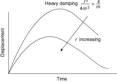
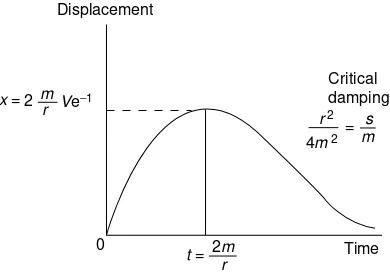
Damped motion of mechanical and electrical oscillators (37) Heavy damping (39) Critical damping (40) Damped simple harmonic oscillations (41) Amplitude decay (43) Logarithmic decrement (44) Relaxation time (46) Energy decay (46)Q-value (46) Rate of energy decay equal to work rate of damping force (48) Summary of important results.
Chapter 3 The Forced Oscillatior
The vector operator i (53) Electrical and mechanical impedance (56) Transient and steady state behaviour of a forced oscillator (58) Variation of displacement and velocity with frequency of driving force (60) Frequency dependence of phase angle between force and (a) displacement, (b) velocity (60) Vibration insulation (64) Power supplied to oscillator (68)Q-value as a measure of power absorption bandwidth (70)Q-value as amplification factor of low frequency response (71) Effect of transient term (74) Summary of important results.
Chapter 4 Coupled Oscillations
Spring coupled pendulums (79) Normal coordinates and normal modes of vibration (81) Matrices and eigenvalues (86) Inductance coupling of electrical oscillators (87) Coupling of many oscillators on a loaded string (90) Wave motion as the limit of coupled oscillations (95) Summary of important results.
Chapter 5 Transverse Wave Motion
Notation of partial differentiation (107) Particle and phase velocities (109) The wave equation (110) Transverse waves on a string (111) The string as a forced oscillator (115) Characteristic impedance of a string (117) Reflection and transmission of transverse waves at a boundary (117) Impedance matching (121) Insertion of quarter wave element (124) Standing waves on a string of fixed length (124) Normal modes and eigenfrequencies (125) Energy in a normal mode of oscillation (127) Wave groups (128) Group velocity (130) Dispersion (131) Wave group of many components (132) Bandwidth Theorem (134) Transverse waves in a periodic structure (crystal) (135) Doppler Effect (141) Summary of important results.
Chapter 6 Longitudinal Waves
Wave equation (151) Sound waves in gases (151) Energy distribution in sound waves (155) Intensity (157) Specific acoustic impedance (158) Longitudinal waves in a solid (159) Young’s Modulus (159) Poisson’s ratio (159) Longitudinal waves in a periodic structure (162) Reflection and transmission of sound waves at a boundary (163) Summary of important results.
Chapter 7 Waves on Transmission Lines
Ideal transmission line (173) Wave equation (174) Velocity of voltage and current waves (174) Characteristic impedance (175) Reflection at end of terminated line (177) Standing waves in short circuited line (178) Transmission line as a filter (179) Propagation constant (181) Real transmission line with energy losses (183) Attenuation coefficient (185) Diffusion equation (187) Diffusion coefficients (190) Attenuation (191) Wave equation plus diffusion effects (190) Summary of important results.
Chapter 8 Electromagnetic Waves
Permeability and permittivity of a medium (199) Maxwell’s equations (202) Displacement current (202) Wave equations for electric and magnetic field vectors in a dielectric (204) Poynting vector (206) Impedance of a dielectric to e.m. waves (207) Energy density of e.m. waves (208) Electromagnetic waves in a conductor (208) Effect of conductivity adds diffusion equation to wave equation (209) Propagation and attenuation of e.m. waves in a conductor (210) Skin depth (211) Ratio of displacement current to conduction current as a criterion for dielectric or conducting behaviour (213) Relaxation time of a conductor (214) Impedance of a conductor to e.m. waves (215) Reflection and transmission of e.m. waves at a boundary (217) Normal incidence (217) Oblique incidence and Fresnel’s equations (218) Reflection from a conductor (222) Connection between impedance and refractive index (219) E.m. waves in plasmas and the ionosphere (223) Summary of important results.
Chapter 9 Waves in More than One Dimension
Plane wave representation in 2 and 3 dimensions (239) Wave equation in 2- dimensions (240) Wave guide (242) Reflection of a 2-dimensional wave at rigid boundaries (242) Normal modes and method of separation of variables for 1, 2 and 3 dimensions (245) Normal modes in 2 dimensions on a rectangular membrane (247) Degeneracy (250) Normal modes in 3 dimensions (250) Number of normal modes per unit frequency interval per unit volume (251) Application to Planck’s Radiation Law and Debye’s Theory of Specific Heats (251) Reflection and transmission of an e.m. wave in 3 dimensions (254) Snell’s Law (256) Total internal reflexion and evanescent waves (256) Summary of important results.
Chapter 10 Fourier Methods
Fourier series for a periodic function (267) Fourier series for any interval (271) Application to a plucked string (275) Energy in normal modes (275) Application to rectangular velocity pulse on a string (278) Bandwidth Theorem (281) Fourier integral of a single pulse (283) Fourier Transforms (285) Application to optical diffraction (287) Dirac function (292) Convolution (292) Convolution Theorem (297) Summary of important results.
Chapter 11 Waves in Optical Systems
Fermat’s Principle (307) Laws of reflection and refraction (307) Wavefront propagation through a thin lens and a prism (310) Optical systems (313) Power of an optical surface (314) Magnification (316) Power of a thin lens (318) Principal planes of an optical system (320) Newton’s equation (320) Optical Helmholtz equation (321) Deviation through a lens system (322) Location of principal planes (322) Matrix application to lens systems (325) Summary of important results.
Chapter 12 Interference and Diffraction
Interference (333) Division of amplitude (334) Fringes of constant inclination and thickness (335) Newton’s Rings (337) Michelson’s spectral interferometer (338) Fabry– Perot interferometer (341) Finesse (345) Resolving power (343) Free spectral range (345) Central spot scanning (346) Laser cavity (347) Multilayer dielectric films (350) Optical fibre wave guide (353) Division of wavefront (355) Two equal sources (355) Spatial coherence (360) Dipole radiation (362) Linear array ofN equal sources (363) Fraunhofer diffraction (367) Slit (368) N slits (370) Missing orders (373) Transmission diffraction grating (373) Resolving power (374) Bandwidth theorem (376) Rectangular aperture (377) Circular aperture (379) Fraunhofer far field diffraction (383) Airy disc (385) Michelson Stellar Interferometer (386) Convolution Array Theorem (388) Optical Transfer Function (391) Fresnel diffraction (395) Straight edge (397) Cornu spiral (396) Slit (400) Circular aperture (401) Zone plate (402) Holography (403) Summary of important results.
Chapter 13 Wave Mechanics
Historical review (411) De Broglie matter waves and wavelength (412) Heisenberg’s Uncertainty Principle (414) Schro¨dinger’s time independent wave equation (417) The wave function (418) Infinite potential well in 1 dimension (419) Quantization of energy (421) Zero point energy (422) Probability density (423) Normalization (423) Infinite potential well in 3 dimensions (424) Density of energy states (425) Fermi energy level (426) The potential step (426) The finite square potential well (434) The harmonic oscillator (438) Electron waves in solids (441) Bloch functions (441) Kronig–Penney Model (441) Brillouin zones (445) Energy band (446) Band structure (448) Phonons (450) Summary of important results.
Chapter 14 Non-linear Oscillations and Chaos
Anharmonic oscillations (459) Free vibrations of finite amplitude pendulum (459) Non-linear restoring force (460) Forced vibrations (460) Thermal expansion of a crystal (463) Electrical ‘relaxation’ oscillator (467) Chaos and period doubling in an electrical ‘relaxation’ oscillator (467) Chaos in population biology (469) Chaos in a non-linear electrical oscillator (477) Phase space (481) Chaos in a forced non-linear mechanical oscillator (487) Fractals (490) Koch Snowflake (490) Cantor Set (491) Smale Horseshoe (493) Chaos in fluids (494) Couette flow (495) Rayleigh–Benard convection (497) Lorenz chaotic attractor. (500) List of references
Chapter 15 Non-linear waves, Shocks and Solitons
Non-linear acoustic effects (505) Shock wave in a gas (506) Mach cone (507) Solitons (513) The KdV equation (515) Solitons and Schro¨dinger’s equation (520) Instantons (521) Optical solitons (521) Bibliography and references.
Appendix 1 Normal Modes, Phase Space and Statistical Physics
Number of phase space ‘cells’ per unit volume (533) Macrostate (535) Microstate (535) Relative probability of energy level population for statistical distributions (a) Maxwell– Boltzmann, (b) Fermi–Dirac, (c) Bose–Einstein (536) Mathematical derivation of the statistical distributions (542).
Appendix 2 Kirchhoff’s Integral Theorem (547) Appendix 3 Non-linear Schro¨dinger Equation (551) Index (553)
1
Simple Harmonic Motion
At first sight the eight physical systems in Figure 1.1 appear to have little in common. 1.1(a) is a simple pendulum, a massmswinging at the end of a light rigid rod of lengthl. 1.1(b) is a flat disc supported by a rigid wire through its centre and oscillating through
small angles in the plane of its circumference.
1.1(c) is a mass fixed to a wall via a spring of stiffness s sliding to and fro in the x direction on a frictionless plane.
1.1(d) is a mass mat the centre of a light string of length 2l fixed at both ends under a constant tensionT. The mass vibrates in the plane of the paper.
1.1(e) is a frictionless U-tube of constant cross-sectional area containing a lengthl of liquid, density, oscillating about its equilibrium position of equal levels in each limb.
1.1(f ) is an open flask of volume Vand a neck of length l and constant cross-sectional area Ain which the air of densityvibrates as sound passes across the neck. 1.1(g) is a hydrometer, a body of massmfloating in a liquid of densitywith a neck of
constant cross-sectional area cutting the liquid surface. When depressed slightly from its equilibrium position it performs small vertical oscillations.
1.1(h) is an electrical circuit, an inductanceLconnected across a capacitanceCcarrying a chargeq.
All of these systems are simple harmonic oscillators which, when slightly disturbed from their equilibrium or rest postion, will oscillate with simple harmonic motion. This is the most fundamental vibration of a single particle or one-dimensional system. A small displacementxfrom its equilibrium position sets up a restoring force which is proportional toxacting in a direction towards the equilibrium position.
Thus, this restoring forceFmay be written F¼ sx
wheres, the constant of proportionality, is called the stiffness and the negative sign shows that the force is acting against the direction of increasing displacement and back towards
1
The Physics of Vibrations and Waves, 6th Edition H. J. Pain
(a) (b)
c
I x
l
θ
m
mx + mg = 0x l ml + mg = 0
.. ..
ω2 = g/ l
mg sin ∼ mg ~
mg x l ~ ~
mg
I + c = 0.. ω2 = c
l
θ θ
θ θ
θ
θ θ
m
x s
(c) (d)
x m
T T
2 l mx + sx = 0
ω2 = s/m
mx + 2T = 0x l
ω2= 2 T l m
. . . .
2x
x x
x
p p
A V
l (f)
(e) p lx + 2 pg x = 0..
ω2 = 2g/l
p Alx + γ pxA2 v = 0
ω2 = γ pAl pV ..
the equilibrium position. A constant value of the stiffness restricts the displacement x to small values (this is Hooke’s Law of Elasticity). The stiffnesssis obviously the restoring force per unit distance (or displacement) and has the dimensions
force distance
MLT2 L
The equation of motion of such a disturbed system is given by the dynamic balance between the forces acting on the system, which by Newton’s Law is
mass times acceleration¼restoring force or
m€xx¼ sx
where the acceleration
€ x x¼d
2 x dt2 This gives
m€xxþsx¼0
c
q
L x
A
m
p
(h) (g)
mx + Apgx = 0..
ω2 = A pg/m
Lq + q c = 0 ..
ω2 = 1
Lc
Figure 1.1 Simple harmonic oscillators with their equations of motion and angular frequencies!of oscillation. (a) A simple pendulum. (b) A torsional pendulum. (c) A mass on a frictionless plane connected by a spring to a wall. (d) A mass at the centre of a string under constant tensionT. (e) A fixed length of non-viscous liquid in a U-tube of constant cross-section. (f ) An acoustic Helmholtz resonator. (g) A hydrometer massmin a liquid of density. (h) An electricalL Cresonant circuit
or
€xxþ s mx¼0 where the dimensions of
s m are
MLT2 ML ¼T
2 ¼2
HereTis a time, or period of oscillation, the reciprocal of which is the frequency with which the system oscillates.
However, when we solve the equation of motion we shall find that the behaviour ofx with time has a sinusoidal or cosinusoidal dependence, and it will prove more appropriate to consider, not, but the angular frequency!¼2 so that the period
T¼1 ¼2
ffiffiffiffi
m s
r
wheres=m is now written as!2. Thus the equation of simple harmonic motion €xxþ s
mx¼0 becomes
€xxþ!2x
¼0 ð1:1Þ
(Problem 1.1)
Displacement in Simple Harmonic Motion
The behaviour of a simple harmonic oscillator is expressed in terms of its displacementx from equilibrium, its velocityxx, and its acceleration_ €xxat any given time. If we try the solution
x¼Acos!t
where A is a constant with the same dimensions as x, we shall find that it satisfies the equation of motion
€xxþ!2x ¼0 for
_ x
x¼ A!sin!t and
€ x
x¼ A!2cos!t
¼ !2x
Another solution
x¼Bsin!t
is equally valid, whereBhas the same dimensions asA, for then _
x
x¼B!cos!t and
€xx¼ B!2sin!t¼ !2x
The complete or general solution of equation (1.1) is given by the addition or superposition of both values forx so we have
x¼Acos!tþBsin!t ð1:2Þ with
€xx¼ !2
ðAcos!tþBsin!tÞ ¼ !2x
whereAandBare determined by the values ofxandxx_at a specified time. If we rewrite the constants as
A¼asin and B¼acos where is a constant angle, then
A2þB2 ¼a2ðsin2þcos2Þ ¼a2 so that
a¼pffiffiffiffiffiffiffiffiffiffiffiffiffiffiffiffiffiA2þB2
and
x¼asincos!tþacossin!t ¼asinð!tþÞ
The maximum value of sin (!tþ) is unity so the constantais the maximum value ofx, known as the amplitude of displacement. The limiting values of sinð!tþÞare1 so the system will oscillate between the values ofx¼ aand we shall see that the magnitude ofa is determined by the total energy of the oscillator.
anticlockwise direction with a constant angular velocity !. Each rotation, as the radius vector sweeps through a phase angle of 2 rad, therefore corresponds to a complete vibration of the oscillator. In the solution
x¼asinð!tþÞ
the phase constant, measured in radians, defines the position in the cycle of oscillation at the timet¼0, so that the position in the cycle from which the oscillator started to move is
x¼asin The solution
x¼asin!t
defines the displacement only of that system which starts from the origin x¼0 at time t¼0 but the inclusion ofin the solution
x¼asinð!tþÞ
wheremay take all values between zero and 2allows the motion to be defined from any starting point in the cycle. This is illustrated in Figure 1.2 for various values of. (Problems 1.2, 1.3, 1.4, 1.5)
Velocity and Acceleration in Simple Harmonic Motion
The values of the velocity and acceleration in simple harmonic motion forx¼asinð!tþÞ are given by
dx
dt ¼xx_ ¼a!cosð!tþÞ φ4
φ3 φ2 φ1
φ1 φ2
φ3
φ4 φ5
φ6 φ0
φ6
φ5= 270° = 90°
= 0
a a
ωt φ x = a Sin(ωt + )
Figure 1.2 Sinusoidal displacement of simple harmonic oscillator with time, showing variation of starting point in cycle in terms of phase angle
and
d2x
dt2 ¼€xx¼ a! 2sin
ð!tþÞ
The maximum value of the velocity a! is called the velocity amplitude and the acceleration amplitudeis given by a!2.
From Figure 1.2 we see that a positive phase angle of =2 rad converts a sine into a cosine curve. Thus the velocity
_ x
x¼a!cosð!tþÞ leads the displacement
x¼asinð!tþÞ
by a phase angle of=2 rad and its maxima and minima are always a quarter of a cycle ahead of those of the displacement; the velocity is a maximum when the displacement is zero and is zero at maximum displacement. The acceleration is ‘anti-phase’ (rad) with respect to the displacement, being maximum positive when the displacement is maximum negative and vice versa. These features are shown in Figure 1.3.
Often, the relative displacement or motion between two oscillators having the same frequency and amplitude may be considered in terms of their phase difference 12 which can have any value because one system may have started several cycles before the other and each complete cycle of vibration represents a change in the phase angle of ¼2. When the motions of the two systems are diametrically opposed; that is, one has
x = a sin(ωt + )
x = aω cos(ωt + ) ωt
ωt
ωt x = −aω2 sin(ωt + ) aω2
aω a
Acceler
ation
x
V
elocity
x
Displacement
x
φ
φ
φ
Figure 1.3 Variation with time of displacement, velocity and acceleration in simple harmonic motion. Displacement lags velocity by=2 rad and israd out of phase with the acceleration. The initial phase constantis taken as zero
x¼ þa whilst the other is at x¼ a, the systems are ‘anti-phase’ and the total phase difference
12¼nrad wherenis anoddinteger. Identical systems ‘in phase’ have
12¼2nrad
where n is any integer. They have exactly equal values of displacement, velocity and acceleration at any instant.
(Problems 1.6, 1.7, 1.8, 1.9)
Non-linearity
If the stiffnesssis constant, then the restoring forceF¼ sx, when plotted versusx, will produce a straight line and the system is said to be linear. The displacement of a linear simple harmonic motion system follows a sine or cosine behaviour. Non-linearity results when the stiffness sis not constant but varies with displacementx (see the beginning of Chapter 14).
Energy of a Simple Harmonic Oscillator
The fact that the velocity is zero at maximum displacement in simple harmonic motion and is a maximum at zero displacement illustrates the important concept of an exchange between kinetic and potential energy. In an ideal case the total energy remains constant but this is never realized in practice. If no energy is dissipated then all the potential energy becomes kinetic energy and vice versa, so that the values of (a) the total energy at any time, (b) the maximum potential energy and (c) the maximum kinetic energy will all be equal; that is
Etotal¼KEþPE¼KEmax¼PEmax
The solutionx¼asin (!tþ) implies that the total energy remains constant because the amplitude of displacementx¼ ais regained every half cycle at the position of maximum potential energy; when energy is lost the amplitude gradually decays as we shall see later in Chapter 2. The potential energy is found by summing all the small elements of worksx.dx (forcesxtimes distancedx)done by the system against the restoring forceover the range zero tox wherex¼0 gives zero potential energy.
Thus the potential energy¼
ðx
0
sxdx¼1 2sx
2
The kinetic energy is given by1 2m_xx
2 so that the total energy E¼12m_xx2þ12sx2
SinceEis constant we have
dE
dt ¼ ðm€xxþsxÞxx_ ¼0 giving again the equation of motion
m€xxþsx¼0
The maximum potential energy occurs atx¼ aand is therefore PEmax¼12sa2
The maximum kinetic energy is
KEmax¼ ð12mxx_2Þmax¼12ma 2!2
½cos2
ð!tþÞmax ¼1
2ma 2!2
when the cosine factor is unity. But m!2
¼s so the maximum values of the potential and kinetic energies are equal, showing that the energy exchange is complete.
The total energy at any instant of time or value of xis E¼12m_xx2þ12sx2
¼1 2ma
2!2
½cos2ð!tþÞ þsin2ð!tþÞ ¼1
2ma 2!2 ¼1
2sa 2
as we should expect.
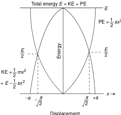
Figure 1.4 shows the distribution of energy versus displacement for simple harmonic motion. Note that the potential energy curve
PE¼1 2 sx
2¼1 2ma
2!2sin2
ð!tþÞ
is parabolic with respect toxand is symmetric aboutx¼0, so that energy is stored in the oscillator both when x is positive and when it is negative, e.g. a spring stores energy whether compressed or extended, as does a gas in compression or rarefaction. The kinetic energy curve
KE¼1 2m_xx
2 ¼1 2ma
2!2cos2ð!tþÞ
is parabolic with respect to bothxandxx. The inversion of one curve with respect to the_ other displays the=2 phase difference between the displacement (related to the potential energy) and the velocity (related to the kinetic energy).
For any value of the displacementx the sum of the ordinates of both curves equals the total constant energyE.
(Problems 1.10, 1.11, 1.12)
Simple Harmonic Oscillations in an Electrical System
So far we have discussed the simple harmonic motion of the mechanical and fluid systems of Figure 1.1, chiefly in terms of the inertial mass stretching the weightless spring of stiffnesss. The stiffnesssof a spring defines the difficulty of stretching; the reciprocal of the stiffness, the complianceC(wheres¼1=C) defines the ease with which the spring is stretched and potential energy stored. This notation of compliance C is useful when discussing the simple harmonic oscillations of the electrical circuit of Figure 1.1(h) and Figure 1.5, where an inductanceLis connected across the plates of a capacitanceC. The force equation of the mechanical and fluid examples now becomes the voltage equation
Energy
Total energy E = KE + PE
E
E 2
E 2
1 2 KE = mx2
1 2 = E − sx2
1 2 PE = sx2
−a a 2
− a
2
+a x
Displacement
Figure 1.4 Parabolic representation of potential energy and kinetic energy of simple harmonic motion versus displacement. Inversion of one curve with respect to the other shows a 90 phase difference. At any displacement value the sum of the ordinates of the curves equals the total constant energyE
I +
+
−
− q
c
Lq + qc = 0 L dI
dt
Figure 1.5 Electrical system which oscillates simple harmonically. The sum of the voltages around the circuit is given by Kirchhoff’s law asLdI=dtþq=C¼0
(balance of voltages) of the electrical circuit, but the form and solution of the equations and the oscillatory behaviour of the systems are identical.
In the absence of resistance the energy of the electrical system remains constant and is exchanged between themagneticfield energy stored in the inductance and theelectricfield energy stored between the plates of the capacitance. At any instant, the voltage across the inductance is
V¼ LdI dt¼ L
d2q dt2
where I is the current flowing and q is the charge on the capacitor, the negative sign showing that the voltage opposes the increase of current. This equals the voltage q=C across the capacitance so that
L€qqþq=C ¼0 ðKirchhoff’s LawÞ or
€ q
qþ!2q¼0 where
!2 ¼ 1
LC
The energy stored in the magnetic field or inductive part of the circuit throughout the cycle, as the current increases from 0 toI, is formed by integrating the power at any instant with respect to time; that is
EL¼
ð
VIdt
(whereVis the magnitude of the voltage across the inductance). So
EL¼
ð
VIdt¼
ð
LdI dtIdt¼
ðI
0 LIdI ¼1
2LI 2¼1
2Lqq_ 2
The potential energy stored mechanically by the spring is now stored electrostatically by the capacitance and equals
1 2CV
2 ¼ q
2
2C
Comparison between the equations for the mechanical and electrical oscillators mechanical (force)!m€xxþsx¼0
electrical (voltage)!L€qqþq C¼0 mechanical (energy)!1
2mxx_ 2þ1
2sx 2¼E
electrical (energy)!1 2Lqq_
2 þ12q
2
C ¼E
shows that magnetic field inertia (defined by the inductanceL) controls the rate of change of current for a given voltage in a circuit in exactly the same way as the inertial mass controls the change of velocity for a given force. Magnetic inertial or inductive behaviour arises from the tendency of the magnetic flux threading a circuit to remain constant and reaction to any change in its value generates a voltage and hence a current which flows to oppose the change of flux. This is the physical basis of Fleming’s right-hand rule.
Superposition of Two Simple Harmonic Vibrations in One
Dimension
(1) Vibrations Having Equal Frequencies
In the following chapters we shall meet physical situations which involve the superposition of two or more simple harmonic vibrations on the same system.
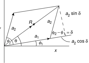
We have already seen how the displacement in simple harmonic motion may be represented in magnitude and phase by a constant length vector rotating in the positive (anticlockwise) sense with a constant angular velocity!. To find the resulting motion of a system which moves in the x direction under the simultaneous effect of two simple harmonic oscillations of equal angular frequencies but of different amplitudes and phases, we can represent each simple harmonic motion by its appropriate vector and carry out a vector addition.
If the displacement of the first motion is given by x1 ¼a1cosð!tþ1Þ and that of the second by
x2 ¼a2cosð!tþ2Þ
then Figure 1.6 shows that the resulting displacement amplitudeRis given by R2 ¼ ða1þa2cosÞ2þ ða2sinÞ2
¼a21þa22þ2a1a2cos where¼21 is constant.
The phase constant of Ris given by
tan ¼ a1sin1þa2sin2 a1cos1þa2cos2 so the resulting simple harmonic motion has a displacement
x¼Rcosð!tþ Þ
an oscillation of the same frequency!but having an amplitudeRand a phase constant .
(Problem 1.13)
(2) Vibrations Having Different Frequencies
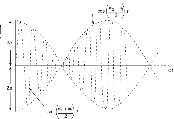
Suppose we now consider what happens when two vibrations of equal amplitudes but different frequencies are superposed. If we express them as
x1 ¼asin!1t and
x2 ¼asin!2t where
!2> !1 y
x a2
a1
R a2
2
a2 sin δ
a2 cos δ 2 − 1 = δ φ θ
φ φ
f1
Figure 1.6 Addition of vectors, each representing simple harmonic motion along the x axis at angular frequency!to give a resulting simple harmonic motion displacementx¼Rcosð!tþ Þ ---here shown fort¼0
then the resulting displacement is given by
x¼x1þx2¼aðsin!1tþsin!2tÞ ¼2asin ð!1þ!2Þt
2 cos
ð!2!1Þt 2
This expression is illustrated in Figure 1.7. It represents a sinusoidal oscillation at the average frequencyð!1þ!2Þ=2 having a displacement amplitude of 2awhich modulates; that is, varies between 2aand zero under the influence of the cosine term of a much slower frequency equal to half the differenceð!2!1Þ=2 between the original frequencies.
When!1 and!2 are almost equal the sine term has a frequency very close to both!1 and!2whilst the cosine envelope modulates the amplitude 2aat a frequency (!2!1)=2 which is very slow.
Acoustically this growth and decay of the amplitude is registered as ‘beats’ of strong reinforcement when two sounds of almost equal frequency are heard. The frequency of the ‘beats’ is ð!2!1Þ, the difference between the separate frequencies (not half the difference) because the maximum amplitude of 2aoccurs twice in every period associated with the frequency (!2!1Þ=2. We shall meet this situation again when we consider the coupling of two oscillators in Chapter 4 and the wave group of two components in Chapter 5.
2a 2a x
ω2 − ω1
2 t
ωt cos
ω2 +ω1
2 t
sin
Figure 1.7 Superposition of two simple harmonic displacementsx1¼asin!1tandx2¼asin!2t
when !2> !1. The slow cos ½ð!2!1Þ=2t envelope modulates the sin ½ð!2þ!1Þ=2t curve
between the valuesx¼ 2a
Superposition of Two Perpendicular Simple Harmonic
Vibrations
(1) Vibrations Having Equal Frequencies
Suppose that a particle moves under the simultaneous influence of two simple harmonic vibrations of equal frequency, one along thexaxis, the other along the perpendicularyaxis. What is its subsequent motion?
This displacements may be written
x¼a1sinð!tþ1Þ y¼a2sinð!tþ2Þ
and the path followed by the particle is formed by eliminating the time t from these equations to leave an expression involving onlyxandyand the constants1 and2.
Expanding the arguments of the sines we have x
a1 ¼
sin!tcos1þcos!tsin1
and
y a2 ¼
sin!tcos2þcos!tsin2 If we carry out the process
x a1
sin2 y a2
sin1
2
þ ay 2
cos1 x a1
cos2
2
this will yield
x2 a21þ
y2 a22
2xy a1a2
cosð21Þ ¼sin2ð21Þ ð1:3Þ
which is the general equation for an ellipse.
In the most general case the axes of the ellipse are inclined to thexandyaxes, but these become the principal axes when the phase difference
21¼ 2 Equation (1.3) then takes the familiar form
x2 a2 1
þy 2
a2 2
¼1
that is, an ellipse with semi-axesa1 anda2.
Ifa1¼a2 ¼athis becomes the circle
x2þy2 ¼a2
When
21 ¼0;2;4; etc: the equation simplifies to
y¼a2 a1 x
which is a straight line through the origin of slopea2=a1. Again for21¼, 3, 5, etc., we obtain
y¼ a2 a1 x
a straight line through the origin of equal but opposite slope.
The paths traced out by the particle for various values of ¼21 are shown in Figure 1.8 and are most easily demonstrated on a cathode ray oscilloscope.
When
21¼0; ;2; etc:
and the ellipse degenerates into a straight line, the resulting vibration lies wholly in one plane and the oscillations are said to beplane polarized.
δ = 0 δ = π
4 δ =
π
2 δ = δ =
π 3
4 π
δ = 5π
4 δ =
π 3
2 δ =
π 7
4 δ = 2π δ = π 4 9
2 − 1 = δ x = a sin (ωt + 1)
y
=
a
sin (
ω
t
+
2
)
φ φ φ
φ
Figure 1.8 Paths traced by a system vibrating simultaneously in two perpendicular directions with simple harmonic motions of equal frequency. The phase angleis the angle by which theymotion leads thexmotion
Convention defines the plane of polarization as that plane perpendicular to the plane containing the vibrations. Similarly the other values of
21
yieldcircular or elliptic polarization where the tip of the vector resultant traces out the appropriate conic section.
(Problems 1.14, 1.15, 1.16)
Polarization
Polarization is a fundamental topic in optics and arises from the superposition of two perpendicular simple harmonic optical vibrations. We shall see in Chapter 8 that when a light wave is plane polarized its electrical field oscillation lies within a single plane and traces a sinusoidal curve along the direction of wave motion. Substances such as quartz and calcite are capable of splitting light into two waves whose planes of polarization are perpendicular to each other. Except in a specified direction, known as the optic axis, these waves have different velocities. One wave, the ordinary or O wave, travels at the same velocity in all directions and its electric field vibrations are always perpendicular to the optic axis. The extraordinary orEwave has a velocity which is direction-dependent. Both ordinary and extraordinary light have their own refractive indices, and thus quartz and calcite are known as doubly refracting materials. When the ordinary light is faster, as in quartz, a crystal of the substance is defined as positive, but in calcite the extraordinary light is faster and its crystal is negative. The surfaces, spheres and ellipsoids, which are the loci of the values of the wave velocities in any direction are shown in Figure 1.9(a), and for a
Optic axis
O vibration
E vibration
x
y
x E ellipsoid O sphere z
y O sphere E ellipsoid
Optic axis
z
Quartz (+ve) Calcite (−ve)
Figure 1.9a Ordinary (spherical) and extraordinary (elliposoidal) wave surfaces in doubly refracting calcite and quartz. In calcite theEwave is faster than theOwave, except along the optic axis. In quartz theOwave is faster. TheOvibrations are always perpendicular to the optic axis, and theOand Evibrations are always tangential to their wave surfaces
This section may be omitted at a first reading.
given direction the electric field vibrations of the separate waves are tangential to the surface of the sphere or ellipsoid as shown. Figure 1.9(b) shows plane polarized light normally incident on a calcite crystal cut parallel to its optic axis. Within the crystal the faster E wave has vibrations parallel to the optic axis, while the O wave vibrations are perpendicular to the plane of the paper. The velocity difference results in a phase gain of the E vibration over the O vibration which increases with the thickness of the crystal. Figure 1.9(c) shows plane polarized light normally incident on the crystal of Figure 1.9(b) with its vibration at an angle of 45 of the optic axis. The crystal splits the vibration into
Plane polarized light normally incident
O vibration to plane of paper
E vibration Optic axis Calcite
crystal
Figure 1.9b Plane polarized light normally incident on a calcite crystal face cut parallel to its optic axis. The advance of theEwave over theOwave is equivalent to a gain in phase
E O 45°
E vibration 90° ahead in phase of O vibration O
E (Optic axis)
Calcite crystal
Optic axis
Phase difference causes rotation of resulting electric field vector Sinusoidal
vibration of electric field
Figure 1.9c The crystal of Fig. 1.9c is thick enough to produce a phase gain of =2 rad in the Ewave over theOwave. Wave recombination on leaving the crystal produces circularly polarized light
equalEandOcomponents, and for a given thickness theEwave emerges with a phase gain of 90 over the O component. Recombination of the two vibrations produces circularly polarized light, of which the electric field vector now traces a helix in the anticlockwise direction as shown.
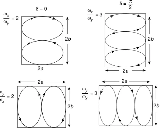
(2) Vibrations Having Different Frequencies(Lissajous Figures)
When the frequencies of the two perpendicular simple harmonic vibrations are not equal the resulting motion becomes more complicated. The patterns which are traced are called Lissajous figures and examples of these are shown in Figure 1.10 where the axial frequencies bear the simple ratios shown and
¼21 ¼0 (on the left) ¼2 (on the right)
If the amplitudes of the vibrations are respectivelyaandb the resulting Lissajous figure will always be contained within the rectangle of sides 2aand 2b. The sides of the rectangle will be tangential to the curve at a number of points and the ratio of the numbers of these tangential points along thexaxis to those along theyaxis is the inverse of the ratio of the corresponding frequencies (as indicated in Figure 1.10).
2a
2b
2b 2a
2b
2a 2a
2b ωx ωy = 3 ωx
ωy = 2
ωy ωx = 3 ωy
ωx = 2
δ = 0
π 2 δ =
Figure 1.10 Simple Lissajous figures produced by perpendicular simple harmonic motions of different angular frequencies
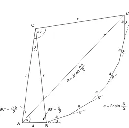
Superposition of a Large Number
n
of Simple Harmonic Vibrations
of Equal Amplitude
a
and Equal Successive Phase Difference
d
Figure 1.11 shows the addition ofnvectors of equal length a, each representing a simple harmonic vibration with a constant phase difference from its neighbour. Two general physical situations are characterized by such a superposition. The first is met in Chapter 5 as a wave group problem where the phase difference arises from a small frequency difference,!, between consecutive components. The second appears in Chapter 12 where the intensity of optical interference and diffraction patterns are considered. There, the superposed harmonic vibrations will have the same frequency but each component will have a constant phase difference from its neighbour because of the extradistanceit has travelled.
The figure displays the mathematical expression
Rcosð!tþÞ ¼acos!tþacosð!tþÞ þacosð!tþ2Þ þ þacosð!tþ ½n1Þ
A
B a
a
a
a a
a a
C r
O
r r
α δ
δ
δ
δ
δ δ
δ δ
90° − 2 90° −
2 n δ
n δ
2 n δ
R = 2 r sin
2 δ a = 2r sin
Figure 1.11 Vector superposition of a large number n of simple harmonic vibrations of equal amplitudeaand equal successive phase difference. The amplitude of the resultant
R¼2rsinn 2 ¼a
sinn=2 sin=2 and its phase with respect to the first contribution is given by
¼ ðn1Þ=2
whereRis the magnitude of the resultant andis its phase difference with respect to the first componentacos!t.
Geometrically we see that each length
a¼2rsin 2
whereris the radius of the circle enclosing the (incomplete) polygon. From the isosceles triangle OAC the magnitude of the resultant
R¼2rsin n 2 ¼a
sinn=2 sin=2 and its phase angle is seen to be
¼OAAB^ OAAC^ In the isosceles triangle OAC
^ O
OAC¼90n2 and in the isosceles triangle OAB
OAAB^ ¼90 2 so
¼ 90 2
90n 2
¼ ðn1Þ 2
that is, half the phase difference between the first and the last contributions. Hence the resultant
Rcosð!tþÞ ¼asinn=2
sin=2 cos !tþ ðn1Þ 2
We shall obtain the same result later in this chapter as an example on the use of exponential notation.
For the moment let us examine the behaviour of the magnitude of the resultant
R¼asinn=2 sin=2
which is not constant but depends on the value of. When nis very large is very small and the polygon becomes an arc of the circle centreO, of lengthna¼A, with Ras the chord. Then
¼ ðn1Þ2n2
and
sin 2!
2
n
Hence, in this limit,
R¼asinn=2 sin=2 ¼a
sin =n ¼na
sin ¼
Asin
The behaviour ofAsin=versus is shown in Figure 1.12. The pattern is symmetric about the value¼0 and is zero whenever sin¼0 except at!0 that is, when sin =!1. When¼0,¼0 and the resultant of thenvectors is the straight line of length A, Figure 1.12(b). AsincreasesAbecomes the arc of a circle until at¼=2 the first and last contributions are out of phase ð2¼Þ and the arc A has become a semicircle of which the diameter is the resultantRFigure 1.12(c). A further increase inincreasesand curls the constant lengthAinto the circumference of a circle (¼) with a zero resultant, Figure 1.12(d). At ¼3=2, Figure 1.12(e) the length A is now 3/2 times the circumference of a circle whose diameter is the amplitude of the first minimum.
Superposition of
n
Equal SHM Vectors of Length
a
with
Random Phase
When the phase difference between the successive vectors of the last section may take random valuesbetween zero and 2(measured from thexaxis) the vector superposition and resultantRmay be represented by Figure 1.13.
(b) (c)
(e) (d)
0
R A
2A
A A=na
A = R =
α α
2π π π
π
2
2 π
2 3
3 circumference A sinα
Figure 1.12 (a) Graph ofAsin= versus , showing the magnitude of the resultants for (b) ¼0; (c)¼/2; (d)¼and (e)¼3/2
This section may be omitted at a first reading.
The components ofRon thexandyaxes are given by
Rx¼acos1þacos2þacos3. . .acosn ¼aX
n
i¼1 cosi
and
Ry¼a
Xn
i¼1 sini
where
R2 ¼R2xþR2y
Now
R2x¼a2 X n
i¼1 cosi
!2
¼a2 X n
i¼1
cos2iþ
Xn
i¼1
i6¼j
cosi
Xn
j¼1 cosj
2
4
3
5
In the typical term 2 cosicosjof the double summation, cosiand cosjhave random values between 1 and the averaged sum of sets of these products is effectively zero.
The summation
Xn
i¼1
cos2i ¼ncos2 R
x y
Figure 1.13 The resultantR¼ ffiffiffi n
p
that is, the number of termsntimes the average value cos2which is the integrated value of cos2 over the interval zero to 2divided by the total interval 2, or
cos2¼ 1 2
ð2
0
cos2d¼12¼sin2
So
R2x ¼a2X n
i¼1
cos2i ¼na2cos2i ¼ na2
2 and
R2y ¼a2X n
i¼1
sin2i ¼na2sin2i¼ na2
2 giving
R2 ¼R2xþR2y ¼na2
or
R¼ ffiffiffi
n p
a
Thus, the amplitude R of a system subjected to n equal simple harmonic motions of amplitudeawith random phases in only ffiffiffi
n p
awhereas, if the motions were all in phaseR would equalna.
Such a result illustrates a very important principle of random behaviour. (Problem 1.17)
Applications
Incoherent Sources in Optics The result above is directly applicable to the problem of coherence in optics. Light sources which are in phase are said to be coherent and this condition is essential for producing optical interference effects experimentally. If the amplitude of a light source is given by the quantityaits intensity is proportional to a2,n coherent sources have a resulting amplitude na and a total intensity n2a2. Incoherent sources have random phases,nsuch sources each of amplitudeahave a resulting amplitude
ffiffiffi
n p
aand a total intensity of na2.
Random Processes and Energy Absorption From our present point of view the importance of random behaviour is the contribution it makes to energy loss or absorption from waves moving through a medium. We shall meet this in all the waves we discuss.
Random processes, for example collisions between particles, in Brownian motion, are of great significance in physics. Diffusion, viscosity or frictional resistance and thermal conductivity are all the result of random collision processes. These energy dissipating phenomena represent the transport of mass, momentum and energy, and change only in the direction of increasing disorder. They are known as ‘thermodynamically irreversible’ processes and are associated with the increase of entropy. Heat, for example, can flow only from a body at a higher temperature to one at a lower temperature. Using the earlier analysis where the length a is no longer a simple harmonic amplitude but is now the average distance a particle travels between random collisions (its mean free path), we see that afternsuch collisions (with, on average, equal time intervals between collisions) the particle will, on average, have travelled only a distance ffiffiffi
n p
afrom its position at timet¼0, so that the distance travelled varies only with the square root of the time elapsed instead of being directly proportional to it. This is a feature of all random processes.
Not all the particles of the system will have travelled a distance ffiffiffi
n p
abut this distance is the most probable and represents a statistical average.
Random behaviour is described by the diffusion equation (see the last section of Chapter 7) and a constant coefficient called the diffusivity of the process will always arise. The dimensions of a diffusivity are always length2/time and must be interpreted in terms of a characteristic distance of the process which varies only with the square root of time.
Some Useful Mathematics
The Exponential SeriesBy a ‘natural process’ of growth or decay we mean a process in which a quantity changes by a constant fraction of itself in a given interval of space or time. A 5% per annum compound interest represents a natural growth law; attenuation processes in physics usually describe natural decay.
The law is expressed differentially as dN
N ¼ dx or dN
N ¼ dt
where N is the changing quantity, is a constant and the positive and negative signs represent growth and decay respectively. The derivatives dN/dx or dN/dt are therefore proportional to the value ofN at which the derivative is measured.
Integration yieldsN¼N0exorN¼N0etwhereN0 is the value atxort¼0 and e is the exponential or the base of natural logarithms. The exponential series is defined as
ex¼1þxþx 2
2!þ x3
3!þ þ xn n!þ
and is shown graphically for positive and negativexin Figure 1.14. It is important to note that whatever the form of the index of the logarithmic base e, it is the power to which the
base is raised, and is therefore always non-dimensional. Thusexis non-dimensional and must have the dimensions ofx1. Writing
ex
¼1þxþðxÞ 2
2! þ ðxÞ3
3! þ it follows immediately that
d dxðe
x
Þ ¼þ2 2
2! xþ 33
3! x 2
þ
¼ 1þxþðxÞ 2
2! þ ðxÞ3
3!
!
þ
" #
¼ex Similarly
d2 dx2ðe
x
Þ ¼2ex
In Chapter 2 we shall use d(et)=dt¼et and d2 (et)=dt2
¼2et on a number of occasions.
By taking logarithms it is easily shown that exey
¼exþy since log
e ðexeyÞ ¼ logeexþlogeey¼xþy.
The Notationi¼ ffiffiffiffiffiffiffi
1
p
The combination of the exponential s