A PARALLEL ALGORITHM FOR COMPUTING THE GROUP
INVERSE VIA PERRON COMPLEMENTATION∗
MICHAEL NEUMANN† AND JIANHONG XU‡
Abstract. A parallel algorithm is presented for computing the group inverse of a singular M–matrix of the formA=I−T, where T ∈Rn×n is irreducible and stochastic. The algorithm is constructed in the spirit of Meyer’s Perron complementation approach to computing the Perron vector of an irreducible nonnegative matrix. The asymptotic number of multiplication operations that is necessary to implement the algorithm is analyzed, which shows that the algorithm saves a significant amount of computation over the direct computation of the group inverse ofA.
Key words. Group inverses, M–matrices, Perron complements, Parallel algorithm.
AMS subject classifications. 15A09, 15A48, 15A51, 65F30, 65C40.
1. Introduction. The group inverse of a matrix A ∈ Rn×n, denoted by A# when it exists, is the unique matrix X ∈ Rn×n that satisfies the matrix equations
AXA =A, XAX =X, and AX =XA. The group inverse has been utilized in a variety of applications [5, 6 , 7, 8, 9, 12, 14, 18, 19, 20, 21, 22, 23, 25, 26 , 30], mostly in the context of a singular M–matrix
(1.1) A=ρSI−S,
whereS ∈Rn×n is nonnegative and irreducible and whereρS is its Perron root.1 In
particular, these applications include:
(i) For a finite ergodic Markov chain with a transition matrixT, Meyer [25] has shown that virtually all the important characteristics of the chain can be determined from the group inverse ofA=ρTI−T =I−T. Furthermore, in [8, 14, 21, 26, 30] it
has been shown that the entries ofA# can be used to provide perturbation bounds on the stationary distribution vector of the chain.
(ii) In [5, 6] it has been shown that for A in (1.1), the signs of the entries of
A# give us qualitative information about the behavior of the Perron root ofS as a function of the entries ofS, namely in addition to it being known that the Perron root is a strictly increasing function of each of the entries, the signs of the entries of
A# answer the question whether the Perron root is a concave or a convex function of each of the entries. Results of this type have been applied in the study of matrix population models in [19, 23].
∗Received by the editors 20 December 2004. Accepted for publication 5 April 2005. Handling
Editor: Ravindra B. Bapat.
†Department of Mathematics, University of Connecticut, Storrs, Connecticut 06269–3009, USA
([email protected]). The work of this author was supported in part by NSF Grant No. DMS0201333.
‡Department of Mathematics and Statistics, University of West Florida, Pensacola, Florida 32514,
USA ([email protected]).
1For such a matrixA, the existence ofA# is guaranteed by the structure of the Jordan blocks
ofS[4, 25].
In view of the above–mentioned applications, a question of interest is how to efficiently compute the group inverseA# ofA in (1.1). Several algorithms for com-puting A# have been suggested in [1, 2, 4, 8, 11, 13, 25]. These methods typically requireO(n3) to O(n4) arithmetic operations and so they can be quite expensive to implement. However, the issue of the parallel computation ofA# has received little attention in the literature.
In this paper we shall present an algorithm for computingA#in parallel, assuming that A is given by (1.1). The numerical evidence which we shall provide indicates that this algorithm is more efficient compared with direct computation ofA#. From the examples that we have tested with MATLAB, the savings in the number of flops (floating point operations) are roughly 50% for matrices of size ranging fromn= 50 to n= 1600. An asymptotic analysis shows that the algorithm saves approximately 12.5% of the multiplication operations if it is implemented in a purely serial fashion. A useful observation is thatAin (1.1) can be reduced, using a diagonal similarity transformation (see, for example, [3, Theorem 2.5.4]), to the case where A := I−
T, with T ∈ Rn×n being irreducible and stochastic. Consequently, without loss of
generality, we shall focus on this case from here on.
The key to constructing our algorithm isPerron complementation. Letαand β
be nonempty subsets of the index setn:={1,2, . . . , n}, both consisting of strictly increasing integers. For anyX∈Rn×n, we shall denote byX[α, β] the submatrix ofX
whose rows and columns are determined byαandβ, respectively. In the special case whenβ =α, we shall use X[α] to denote X[α, α].2 Given the irreducible stochastic matrixT ∈Rn×n, thePerron complementofT[α] is defined to be3
(1.2) Pα:=T[α] +T[α,n\α](I−T[n\α])−1T[n\α, α].
Meyer [27, 28] proved that the Perron complementPα resemblesT. Specifically,
Pα is also irreducible and stochastic and, in addition, on letting π ∈ Rn be the
normalized left Perron vector ofT, viz. the column vector satisfying
(1.3) πtT = πt and π1 = 1,
then
(1.4) πα =
π[α]
ξα
, with ξα = π[α]1,
whereπ[α] is the subvector ofπdetermined byα, turns out to be the normalized left Perron vector of Pα. Based on these results, Meyer introduced a parallel algorithm
for computing the left Perron vector via Perron complementation.
Note that the irreducible stochastic matrixT can be thought of as the transition matrix of some finite ergodic Markov chain{Xi}∞i=0 on state spaceS={1,2, . . . , n}.
2We follow the notation in [15] for submatrices. This notation allows conclusions to be readily
extended to the case whenαandβconsist of nonconsecutive integers.
3The notion of Perron complement can be similarly defined on an irreducible nonnegative matrix
Themean first passage timefrom statesito j, denoted bymi,j, is defined to be the
expected number of time steps that the chain, starting initially from state i, would take before it reaches statej for the first time [17], i.e.
(1.5) mi,j:= E(Fi,j) = ∞
k=1
kPr(Fi,j =k),
whereFi,j := min{ℓ≥1 : Xℓ=j|X0 =i}. The matrixM = [mi,j]∈Rn×n is called
themean first passage matrixof the chain or, simply, ofT. Obviously the mean first
passage matrix of the Perron complementPα can be similarly defined sincePα can
also be regarded as the transition matrix of an ergodic chain with fewer states. As a further development of Meyer’s results on Perron complementation, Kirk-land, Neumann, and Xu [22] showed that the mean first passage matrix ofPαis closely
related toM[α] andM[n\α], i.e. the corresponding submatrices of the mean first passage matrix ofT. Accordingly, the mean first passage matrix of the entire chain can be computed in parallel via Perron complementation.
The interesting relationship between the irreducible stochastic matrixT and its Perron complementPα, as shown in [22, 27, 28], leads us to explore if Perron
com-plementation can be exploited for the parallel computation ofA#. Specifically, on letting Bα :=I−Pα, we ask the following questions: (i) How are A# and B#α
re-lated? (ii) Does the connection between A# and B#
α allow the computation of A#
to be carried out in parallel? These questions will be completely answered in this paper. We point out that the relationship betweenA#[α] andB#
α has been shown in
[29] for the special case whenα={1,2, . . . , n−1}. Furthermore, for the special case whenT is periodic, Kirkland [18] has developed, without recourse to the terminology of Perron complementation, formulae for the blocks ofA#. Thus our results here will also generalize those in [18, 29].
The plan of this paper is as follows. In Section 2 we shall summarize some necessary results on Perron complementation from the literature. Our main results on the computation of the group inverse via Perron complementation will be presented in Section 3. Section 4 will be devoted to describing our parallel algorithm for computing the group inverse. Finally, some concluding remarks are given in Section 5.
2. Preliminaries. Recall that the purpose of this paper is the computation in parallel of the group inverse of A := I−T, where T ∈ Rn×n is irreducible and stochastic.
PartitionT into ak×k(k≥2) block form as follows:
(2.1) T =
T[α1] T[α1, α2] · · · T[α1, αk]
T[α2, α1] T[α2] · · · T[α2, αk]
..
. ... . .. ...
T[αk, α1] T[αk, α2] · · · T[αk]
,
whereα1, α2, . . . , αk are nonempty disjoint subsets of the index setn:={1, . . . , n}
T normalized so thatπ1= 1 and wheree∈Rn is a column vector of all ones. The
vector π is the stationary distribution vector of the underlying Markov chain. Let
M ∈Rn×n be the mean first passage matrix ofT as defined in (1.5). We shall always
partitionA#,W, and M in conformity withT.
Throughout the sequel, the lettersJ andewill represent a matrix of all ones and a column vector of all ones, respectively, whose dimensions can be determined from the context. For any square matrix X, we shall denote byXd the diagonal matrix
obtained fromX by setting all its off–diagonal entries to zero. We begin with the following two lemmas from [4, 25].
LEMMA 2.1. ([4, Theorem 8.5.5])
(2.2) πtA# = 0.
LEMMA 2.2. ([25, Theorem 3.3])The mean first passage matrixM ofT can be
expressed as
(2.3) M = I−A#+J(A#)
d (Wd)−1.
Lemma 2.2 gives the relationship between M and A#. For i = 1,2, . . . , k, let
Pαi be the Perron complement ofT[αi]. In what follows, we shall use the subscript
αi to denote quantities associated withPαi. Put Bαi :=I−Pαi. SincePαi is also
irreducible and stochastic, its mean first passage matrixMαi is defined in the same
way asM. Letπαi be the normalized left Perron vector ofPαi and setWαi :=eπαit .
The following corollary from Lemma 2.2 characterizes the relationship betweenMαi
andB#
αi.
COROLLARY 2.3. For i = 1,2, . . . , k, the mean first passage matrix Mαi of
Pαi can be expressed as
(2.4) Mαi =
I−Bαi#+J(B
#
αi)d [(Wαi)d]−1.
As already mentioned earlier, according to Meyer [27, Theorem 2.1], for i = 1,2, . . . , k, the normalized left Perron vector ofPαi is given by
(2.5) παi =
π[αi]
ξαi
with ξαi =π[αi]1. The number ξαi is called the i–thcoupling factor. Note that k
i=1ξαi = 1. The next lemma, again due to Meyer, points out how the coupling
factors can be obtained without actually computingπ.
LEMMA 2.4. ([27, Theorem 3.2]) Let C= [ci,j]∈Rk×k be defined via
(2.6) ci,j: = παit T[αi, αj]e, i, j= 1,2, . . . , k.
Then C is irreducible and stochastic. Moreover, ξ = [ξα1, ξα2, . . . , ξαk]t is the
The matrixC is called thecoupling matrix.
In the sequel we shall also require the following two lemmas from Kirkland, Neu-mann, and Xu [22] on the relationship betweenM andMαi, the mean first passage
matrix of Pαi. In the first lemma the principal submatrices of M are determined,
while in the second lemma, the off–diagonal blocks ofM are determined.
LEMMA 2.5. ([22, Theorem 2.2])Fori= 1,2, . . . , k,
(2.7) M[αi] =
1
ξαi
Mαi+Vαi,
where
Vαi :=Bαi#T[αi,n\αi](I−T[n\αi])−1J
−B#αiT[αi,n\αi](I−T[n\αi])−1J t
.
(2.8)
The matrixVαi is clearly skew–symmetric and of rank at most 2.
LEMMA 2.6. ([22, Theorem 2.3])Fori= 1,2, . . . , k,
M[n\αi, αi] = (I−T[n\αi])−1
T[n\αi, αi]M[αi] +J
−T[n\αi, αi](M[αi])d .
(2.9)
We comment that Corollary 2.3, formula (2.5), and Lemmas 2.4, 2.5, and 2.6 continue to hold even when any subsetαi consists of nonconsecutive indices.
3. Main Results. In this section we develop our main results in which we show how the blocks of A#, where A := I−T with T ∈ Rn×n being irreducible
and stochastic, can be linked to the group inverses associated with the smaller size irreducible transition matrices arising from Perron complementation. Again we use a
k×k partitioning ofT which is given by (2.1). We construct a matrixU ∈Rn×n by
(3.1) U := (M−Md)Wd,
where, as defined in the previous section, M is the mean first passage matrix ofT
and W := eπt. As we shall see, U turns out to play a central role in establishing
the connection betweenA#and quantities related to Perron complementation and in constructing our parallel algorithm for computingA#. It should be noted thatU is known in the literature to have several interpretations concerning Markov chains and concerning surfing the Web. First, Kemeny and Snell [17, Theorem 4.4.10] observed thatUhas constant row sums
j=iπjmi,j = tr(A#), fori= 1,2, . . . , n. The quantity
entered because of being lost, and enter another random site (see Levene and Loizou [24]). It is also called theexpected time to mixing in a Markov chain(see Hunter [16]). The relationship between the diagonal entries ofA#andU is given by the lemma below, which shows that the diagonal entries of A# can be expressed in terms ofU as well asξαi andπαi arising from Perron complementation.
LEMMA 3.1. Let A#= [a#
i,j]. Then
(3.2) [a#1,1, a # 2,2, . . . , a
#
n,n] = [ξα1πtα1, ξα2παt2, . . . , ξαkπtαk]U.
Proof. First we observe that from Lemma 2.2, mi,i = 1/πi, for all i, i.e. Md =
(Wd)−1.
Next, again by Lemma 2.2, we obtain that
πtU = πt(M −M d)Wd
= πt[I−A#+J(A#)
d](Wd)−1−(Wd)−1 Wd
= −πtA#+πtJ(A#)
d
= [a#1,1, a # 2,2, . . . , a
#
n,n],
where the last equality is due to Lemma 2.1. This, together with (2.5), yield (3.2). Suppose next thatA#andU are partitioned in conformity withT in (2.1). Our next lemma concerns the relationship between the blocks ofA#and those ofU.
LEMMA 3.2. Fori= 1,2, . . . , k,
(3.3) −A#[αi] +J(A#[αi])d=U[αi]
and
(3.4) −A#[n\α
i, αi] +J(A#[αi])d=U[n\αi, αi].
Proof. Similar to the proof of Lemma 3.1, we see that
U = [I−A#+J(A#)
d](Wd)−1−(Wd)−1 Wd
= −A#+J(A#)
d.
that
U[α1] U[α1, β]
U[β, α1] U[β]
= −
A#[α1] A#[α 1, β]
A#[β, α1] A#[β]
+
J(A#[α1])
d J(A#[β])d
J(A#[α1])
d J(A#[β])d
,
from which (3.3) and (3.4) follow.
We are now in a position to introduce our main results. For that purpose recall thatPαi is the Perron complement ofT[αi],Bαi :=I−Pαi,ξαi is thei–th coupling
factor,Wαi :=eπαit , whereπαi is the normalized left Perron vector ofPαi, andVαi is
the skew–symmetric matrix given in (2.8). In Lemma 3.2 we showed how the blocks of A# are related to the corresponding blocks of U. We shall show next how the blocks of U can be obtained from the group inverses of theBαi’s starting with the
diagonal blocks ofU.
THEOREM 3.3. Fori= 1,2, . . . , k,
(3.5) U[αi] = −Bαi# +J(B
#
αi)d+ξαiVαi(Wαi)d.
Proof. It suffices to show the conclusion for the case wheni= 1. By Lemma 2.2
and on partitioningM,A#, andW in conformity withT, we have, using (2.5), that
M[α1] =I−A#[α1] +J(A#[α1])
d [(W[α1])d]−1
= 1
ξα1
I−A#[α1] +J(A#[α1])d [(Wα1)d] −1
.
(3.6)
On the other hand, by (2.4) and (2.7), we find that
(3.7) M[α1] = 1
ξα1
I−B#α1+J(B
#
α1)d [(Wα1)d]−1+Vα1.
It thus follows from (3.6) and (3.7) that
1
ξα1
−A#[α1] +J(A#[α1])
d [(Wα1)d]−1 =
1
ξα1
−B#
α1+J(B
#
α1)d [(Wα1)d] −1+V
α1,
which, by (3.3), can be reduced to
U[α1] = −A#[α1] +J(A#[α1])
d
= −B#
α1+J(Bα#1)d+ξα1Vα1(Wα1)d.
Having determined a representation for the diagonal blocks of U, we now deter-mine a representation for the off–diagonal blocks ofU.
THEOREM 3.4. Fori= 1,2, . . . , k,
(3.8) U[n\αi, αi] = (I−T[n\αi])−1
T[n\αi, αi]U[αi] +ξαiJ(Wαi)d .
Proof. It suffices for the sake of simplicity to set i= 1 and β =n\α1. Thus
what we need to show is the following:
U[β, α1] = (I−T[β])−1T[β, α1]U[α1] +ξ
α1J(Wα1)d .
Again, by Lemma 2.2 and on partitioningM,A#, andW in conformity withT, we have, using (2.5), that
M[β, α1] =−A#[β, α1] +J(A#[α1])
d [(W[α1])d]−1
= 1
ξα1
−A#[β, α1] +J(A#[α1])
d [(Wα1)d]−1.
(3.9)
On the other hand, by (2.4) and (2.7), we see that
M[α1]−(M[α1])d=
1
ξα1
Mα1−(Mα1)d +Vα1
= 1
ξα1
−B#α1+J(B
#
α1)d [(Wα1)d]−1+Vα1,
which, together with (2.9), yield that
M[β, α1] = 1
ξα1
(I−T[β])−1T[β, α1][−B#
α1+J(B
#
α1)d][(Wα1)d]−1
+ξα1T[β, α1]Vα1+ξα1J
= 1
ξα1
(I−T[β])−1T[β, α1]U[α1] +ξ
α1J(Wα1)d [(Wα1)d]−1.
(3.10)
The conclusion follows now from (3.4), (3.9), and (3.10).
THEOREM 3.5. Fori= 1,2, . . . , k, the diagonal blocks of A# are given by:
(3.11)
A#[α
i] = e[ξα1πtα1, ξα2παt2, . . . , ξαkπtαk]U[n, αi]−U[αi]
= e
k
ℓ=1
ξαℓπtαℓ U[αℓ, αi]−U[αi].
The off–diagonal blocks of A# are given as follows: forj=i,1≤i, j≤k,
(3.12) A#[α
j, αi] = e k
ℓ=1
ξαℓπαℓt U[αℓ, αi]−U[αj, αi].
Proof. From (3.3) we know that
A#[αi] =J(A#[αi])d−U[αi].
On the other hand, from (3.2), we have that
(3.13) J(A#[α
i])d=e[ξα1πtα1, ξα2παt2, . . . , ξαkπtαk]U[n, αi].
Thus (3.11) follows.
Similarly, using (3.4) and (3.13), we see that (3.12) holds.
Theorems 3.3, 3.4, and 3.5 clearly illustrate how the blocks ofA# can be assem-bled from quantities arising from Perron complementation, namely fromξαi,παi,Vαi,
andB#
αi. In the next section we shall use this important fact to construct a parallel
algorithm for computingA#.
We comment that according to [29, Formulae (7) and (19)], ifα1 is chosen to be {1,2, . . . , n−1}, then
(3.14) A#[α1] = F+ξα1
µWα1−F Wα1−Wα1F
and
(3.15) B#
α1 = F+
µ ξα1
Wα1−F Wα1−Wα1F,
where F = (I−T[α1])−1 and where µ=ξ
α1πtα1F e. This result, which implies the
close connection betweenA#[α1] and B#
α1, can be regarded as a special case of our
Theorems 3.3, 3.4, and 3.5.
Consider the case when T is not only irreducible and stochastic, but also d– periodic, that is,
(3.16) T =
0 T1 0 · · · 0 0 0 T2 0 · · · 0
..
. ... . .. ... ... ... ..
. ... . .. ... 0
0 0 · · · . .. Td−1
where the diagonal zero blocks are square and where (I−T)# is partitioned con-formably withT in (3.16). For this case Kirkland [18, Theorem 1] has shown how to compute the blocks of (I−T)# in terms of (I−P
j)#, whereP1:=T1T2· · ·Td and
where, for j = 2,3, . . . , d, Pj := TjTj+1· · ·TdT1· · ·Tj−1. It can be readily verified
that for eachj,Pj is indeed the Perron complement of thej–th diagonal block ofT.
This result can also be regarded as a particular case of our Theorems 3.3, 3.4, and 3.5.
We finally remark that Theorems 3.3, 3.4, and 3.5 apply to the case when anyαi
consists of nonconsecutive, but increasing, indices, provided thatα1, α2, . . . , αk form
a partition ofn.
4. Parallel Algorithm. In this section we shall provide a parallel algorithm for the efficient computation ofA# via Perron complementation. The algorithm will be illustrated mainly by partitioningT into a 2×2 block matrix as follows:
(4.1) T =
T[α1] T[α1, α2]
T[α2, α1] T[α2]
,
whereα1and α2, both nonempty, form a partition ofn.
We begin the procedure by computing the Perron complements Pα1 and Pα2.
According to (1.2), this requires certain matrix inversions. We retain the results of these inversions since they will be needed later in the computation ofVα1, Vα2, and
in the computation of the off–diagonal blocks ofU (see (2.8) and (3.8), respectively) too. As shown in the proof of Theorem 3.5, the blocks ofA# are determined by the blocks ofU, the coupling factorsξα1 andξα2, and the normalized left Perron vectors
πα1 andπα2. Among these quantities, eachπαi can be computed separately from its
respectivePαi, whileξα1 and ξα2 can be obtained from the coupling matrix C once
πα1 andπα2 are known.
Continuing, concerning the blocks ofU, each diagonal blockU[αi] is determined
by B#
αi, Vαi, ξαi, and Wαi according to (3.5). Clearly each B#αi can be computed
separately from the corresponding Pαi. As soon as B#αi becomes available, Vαi can
be obtained immediately from (2.8). Having foundU[αi], we proceed with (3.8) so as
to determineU[n\αi, αi].
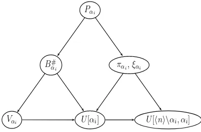
In summary, with a 2×2 partitioning scheme and Perron complementation, the computation of A# can be implemented by computing the following components roughly in the order as they appear: (i)Pα1 andPα2; (ii)πα1 andπα2; (iii)Bα#1 and
B#
α2; (iv)C,ξα1, andξα2; (v)Vα1 andVα2; (vi)U[α1] andU[α2]; and (vii)U[α2, α1] and U[α1, α2]. Each of these components, except (iv), consists of two separate sub-components that can be computed concurrently and in parallel. In addition, steps (ii) and (iii) may also be executed in parallel. The flow of the computation on each
Pαi, as illustrated in Figure 4.1, can obviously be carried out independently, with the
computation ofξα1 andξα2 being the only exception.
Pαi
B#
αi παi,ξαi
[image:11.595.188.386.150.280.2]Vαi U[αi] U[n\αi, αi]
Fig. 4.1.Computation on the Perron ComplementPαi
complements Pαi for i = 1,2, . . . , k, then for each i we proceed to calculating Bαi#,
παi and ξαi, Vαi, U[αi], and U[n\αi, αi] in the order as shown in Figure 4.1, and
finally we recover the blocks ofA# using formulae (3.11) and (3.12). Alternatively, similar to what was suggested in [27], a higher level partitioning scheme can also be achieved by following successive lower level partitionings on the Perron complements. For example, we may partition T into a 2×2 block form and construct the Perron complements Pα1 and Pα2, but then for eachi, we may compute the group inverse
B#
αi using our parallel algorithm by further partitioning the correspondingPαi into a
2×2 block form. In other words, we may computeB#
αi on the Perron complements
ofPαi, rather than directly computing it onPαi.
It is natural to ask whether the above parallel algorithm for computing A# via Perron complementation is less costly than the direct computation ofA#, considering that there are quite a few quantities, though all are smaller thannin size, to compute. To answer this question, we shall estimate the asymptotic number of multiplications necessary to implement the parallel algorithm and compare it with the case without parallelism.
It should be mentioned that for general matrices, there are actually very few numerically viable methods for computingA# because of the issue of numerical in-stability. Specifically, problems might arise in determining the bases for R(A) and
N(A) ([2, 4]) or the characteristic polynomial of A and the resolvent (zI −A)−1 ([11, 13]). Under our assumption on A, namely that A is an irreducible singular M–matrix, however, there is a quite reliable method for computing A# proposed by Meyer [25, Section 5], which can be implemented using the conventional Gaussian eliminations on nonsingular matrices. Here we shall adopt this method while counting the asymptotic numbers of multiplications.
According to Meyer [25, Theorem 5.5 and Table 2], if A# is computed directly from the formula
(4.2) A# = (A+W)−1−W
Suppose now that n= 2m and that α1 ={1,2, . . . , m} and α2 ={m+ 1, m+ 2, . . . , n}. As shown in Figure 4.1, the total number of multiplications required for the computation on eachPαi can be counted as follows:
(i) Pαi. To find (I−T[n\αi])−1T[n\αi, αi], it requires 4m3/3 multiplications
to solve the matrix equation (I−T[n\αi])X =T[n\αi, αi] with Gaussian
eliminations. An additional amount ofm3multiplications is then needed to premultiply (I−T[n\αi])−1T[n\αi, αi] byT[αi,n\αi].
(ii) παi andB#αi. Based on the result in [25], it requires 4m3/3 multiplications
ifπαi is computed first and thenB#αi is computed from a formula similar to
(4.2). We comment that the computation ofξα1 and ξα2 is trivial and does
not requireO(m3) multiplications.
(iii) Vαi. Due to the particular structure ofVαi, it is enough to compute the first
column of the rank–one matrix B#
αiT[αi,n\αi](I−T[n\αi])−1J. This
does not requireO(m3) multiplications since the LU factorization in (i) can be retained.
(iv) U[αi]. Clearly this does not requireO(m3) multiplications.
(v) U[n\αi, αi]. The computation ofξαi(I−T[n\αi])−1J(Wαi)d does not
re-quireO(m3) multiplications for exactly the same reason as mentioned in (iii). It requiresm3 multiplications, however, to postmultiply (I−T[n\α
i])−1×
T[n\αi, αi] byU[αi].
(vi) A#[α
i] and A#[n\αi, αi]. These can be obtained without multiplication
operations from (3.3) and (3.4), respectively, whenJ(A#[α
i])dis known. Note
that, according to (3.13), the computation of J(A#[α
i])d does not require
O(m3) multiplications.
From (i) through (vi), we conclude that the number of multiplications necessary for implementing the parallel algorithm for computingA#is roughly 28m3/3 = 7n3/6. On the other hand, to computeA#directly from (4.2) requires 4n3/3 = 8n3/ 6mul-tiplications. Therefore the parallel algorithm actually saves approximately 1/8 or 12.5% of multiplication operations.
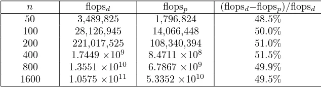
n flopsd flopsp (flopsd−flopsp)/flopsd
[image:12.595.133.450.508.594.2]50 3,489,825 1,796,824 48.5% 100 28,126,945 14,066,448 50.0% 200 221,017,525 108,340,394 51.0% 400 1.7449×10⁹ 8.4711×10⁸ 51.5% 800 1.3551×10¹⁰ 6.7867×10⁹ 49.9% 1600 1.0575×10¹¹ 5.3352×10¹⁰ 49.5%
Table 1: Results of Numerical Tests
We have tested with MATLAB several examples using randomly generated dense matrices and counted the number of flops with MATLAB’s built–in functionflops. The results are given in Table 1, where flopsp stands for the total number of flops
used in the parallel algorithm for computing A#, while flops
d stands for that from
directly computingA# by (4.2).
a reduced amount of computation4. The savings shown in the table are much greater than the asymptotic estimate of a 12.5% reduction in the number of multiplications. The reason appears to be that we have only tested matrices of small to moderate size. There may be also some dependency on the manner in which MATLAB performs matrix operations (multiplications and additions) at machine level.
Finally we make a few comments on the numerical accuracy of our parallel al-gorithm. Our parallel algorithm basically involves two main tasks: to compute the Perron complementsPαiand to compute the group inversesBαi# associated with those
Perron complements. For the same reason as we mentioned earlier, Meyer’s method in [25] is advisable for computing theB#
αi’s. This method can be carried out with
Gaus-sian eliminations as an inversion algorithm on the nonsingular matricesBαi +Wαi
and therefore the standard results on round–off analysis of Gaussian eliminations (see, for example, [10]) apply. It should be noted that compared with that ofA+W in (4.2), the inversion ofBαi+Wαi tends to be more stable because of the reduced size
of the problem [10, Theorem 3.3.1]. In addition, according to [29], the computation ofπαi onPαi tends to be more stable than that of πonT; in particular, the bound
on the relative errors inπαi does not exceed that inπ. On the other hand, Gaussian
eliminations can also be used to invert the matricesI−T[αi] arising from Perron
com-plementation. Even though such nonsingular principal submatrices ofI−T could be poorly conditioned [8], various partitioning schemes may be exploited so as to allevi-ate possible numerical difficulties in calculating (I−T[αi])−1. Consider, for example,
the following 4×4 irreducible stochastic matrix:
T =
.4332 .5667 .0001 .0000
.4331 .5668 .0000 .0001
.0000 .0001 .3667 .6332
.0001 .0000 .3668 .6331
.
Using the condition numberκ∞(X) :=X∞X−1∞, whereX∈Rn×nis
nonsingu-lar, we obtain that forα1={1,2}andα2={3,4},κ∞(I−T[α1])≈1.1335×10⁴and κ∞(I−T[α2])≈1.2665×10⁴, but forα1={1,3}andα2={2,4},κ∞(I−T[α1])≈
1.1175 andκ∞(I−T[α2])≈1.1810.
5. Concluding Remarks. The goal of this paper was to present an efficient parallel algorithm for computing the group inverse of the singular M–matrix A =
I−T, whereT is an irreducible stochastic matrix, via Perron complementation. This algorithm can be easily modified to handle the more general case thatA=ρSI−S,
whereS is an irreducible nonnegative matrix and whereρS is the Perron root ofS.
As shown in Theorems 3.3, 3.4, and 3.5, the group inverse ofAis closely related to the group inverses associated with the Perron complements of T. This adds to previous computational utilization of Perron complementation due to Meyer [27, 28] and Kirkland, Neumann, and Xu [22]. It remains an interesting question whether the Perron complementation approach is applicable to other computational problems relating to irreducible stochastic matrices.
4We remark, however, that the flop–count in the table also reflects the fact that our experiments
In this paper we have focused on implementing the parallel algorithm for com-puting the group inverse ofAwith a 2×2 partitioning scheme. We therefore remark that even though any 2×2 block–partitioning may be used, numerically it is more efficient to chooseαi andn\αi of roughly the same size since it balances the
work-load between the processors. To see this note that as the size ofαidecreases, it is less
costly to compute (I−T[αi])−1, but at the same time, the size of n\αi increases
accordingly, and therefore it is more costly to compute (I−T[n\αi])−1.
The operational count presented in Table 1 shows that the parallel algorithm is capable of significantly reducing the amount of necessary multiplication operations as compared with directly computing the group inverse of A. It is interesting to observe that in [22], the computation of the mean first passage matrix of a finite ergodic Markov chain with transition matrixT is carried out in parallel on the Perron complements of T. A crucial step there is the computation of the group inverse associated with each Perron complement. When this step is accomplished with the parallel algorithm for computingA#developed here, we can expect that in the parallel computation of the mean first passage matrix as suggested in [22], further reductions in the computational effort can be achieved.
REFERENCES
[1] K. M. Anstreicher and U. G. Rothblum. Using Gauss–Jordan elimination to compute the index, generalized nullspaces, and Drazin inverses. Lin. Alg. Appl., 85:221–239, 1987.
[2] A. Ben–Israel and T. N. E. Greville. Generalized Inverses: Theory and Applications, 2nd ed. Springer, New York, 2003.
[3] A. Berman and R. J. Plemmons. Nonnegative Matrices in the Mathematical Sciences. SIAM, Philadelphia, 1994.
[4] S. L. Campbell and C. D. J. Meyer. Generalized Inverses of Linear Transformations. Dover Publications, New York, 1991.
[5] E. Deutsch and M. Neumann. Derivatives of the Perron root at an essentially nonnegative matrix and the group inverse of an M–matrix.J. Math. Anal. Appl., 102:1–29, 1984. [6] E. Deutsch and M. Neumann. On the first and second order derivatives of the Perron vector.
Lin. Alg. Appl., 71:57–76, 1985.
[7] M. Eiermann, I. Marek, and W. Niethammer. On the solution of singular linear equations by semiiterative equations.Numer. Math., 53:265–283, 1988.
[8] R. Funderlic and C. D. Meyer. Sensitivity of the stationary distribution vector for an ergodic Markov chain.Lin. Alg. Appl., 76:1–17, 1986.
[9] G. Golub and C. D. Meyer. Using the QR factorization and group inversion to compute, differentiate, and estimate the sensitivity of stationary probabilities for Markov chains.
SIAM J. Alg. Disc. Meth., 7:273–281, 1986.
[10] G. Golub and C. Van Loan. Matrix Computation, 3rd ed. The John Hopkins Univ. Press, Baltimore, Maryland, 1996.
[11] T. N. E. Greville. The Souriau–Frame algorithm and the Drazin pseudoinverse. MRC. Tech. Sum. Rep., 1182, 1972.
[12] M. Hanke and M. Neumann. Preconditionings and splitting for singular systems. Numer. Math., 57:85–89, 1990.
[13] R. E. Hartwig. More on the Souriau–Frame algorithm and the Drazin inverses. SIAM J. Appl. Math., 31:42–46, 1976.
[14] M. Haviv and L. Van der Heyden. Perturbation bounds for the stationary probabilities of a finite Markov chain.Adv. Appl. Prob., 16:804–818, 1984.
[16] J. J. Hunter. Mixing times with applications to perturbed Markov chains. Preprint, Massey Univ., Auckland, New Zealand, 2003.
[17] J. G. Kemeny and J. L. Snell. Finite Markov Chains. Van Nostrand, Princeton, New Jersey, 1960.
[18] S. J. Kirkland. The group inverse associated with an irreducible periodic nonnegative matrix.
SIAM J. Matrix Anal. Appl., 16:1127–1134, 1995.
[19] S. J. Kirkland and M. Neumann. Convexity and concavity of the Perron root and vector of Leslie matrices with applications to a population model. SIAM J. Matrix Anal. Appl., 15:1092–1107, 1994.
[20] S. J. Kirkland and M. Neumann. Cutpoint decoupling and first passage times for random walks on graphs. SIAM J. Matrix Anal. Appl., 20:860–870, 1999.
[21] S. J. Kirkland, M. Neumann, and B. Shader. Application of Paz’s inequality to perturbation bounds for Markov chains. Lin. Alg. Appl., 268:183–196, 1998.
[22] S. J. Kirkland, M. Neumann, and J. Xu. A divide and conquer approach to computing the mean first passage matrix for Markov chains via Perron complement reduction. Numer. Lin. Alg. Appl., 8:287–295, 2001.
[23] S. J. Kirkland, M. Neumann, and J. Xu. Convexity and elasticity of the growth rate in size– classified population models. SIAM J. Matrix Anal. Appl., 26:170–185, 2004.
[24] M. Levene and G. Loizou. Kemeny’s constant and the random surfer. Amer. Math. Month., 109:741–745, 2002.
[25] C. D. J. Meyer. The role of the group generalized inverse in the theory of finite Markov chains.
SIAM Rev., 17:443–464, 1975.
[26] C. D. Meyer. The condition of a finite Markov chain and perturbation bounds for the limiting probabilities. SIAM J. Alg. Disc. Meth., 1:273–283, 1980.
[27] C. D. Meyer. Uncoupling the Perron eigenvector problem. Lin. Alg. Appl., 114/115:69–94, 1989.
[28] C. D. Meyer. Stochastic complementation, uncoupling Markov chains, and the theory of nearly reducible systems. SIAM Rev., 31:240–272, 1989.
[29] M. Neumann and J. Xu. On the stability of the computation of the stationary probabilities of Markov chains using Perron complements. Numer. Lin. Alg. Appl., 10:603–618, 2003. [30] E. Seneta. Sensitivity analysis, ergodicity coefficients, and rank–one updates for finite Markov