El e c t r o n ic
Jo ur n
a l o
f P
r o b
a b i l i t y
Vol. 9 (2004), Paper no. 24, pages 710-769.
Journal URL
http://www.math.washington.edu/∼ejpecp/
Gaussian Scaling for the Critical Spread-out Contact Process above the Upper Critical Dimension
Remco van der Hofstad1 and Akira Sakai2
Abstract: We consider the critical spread-out contact process in Zd with d≥1, whose infection range
is denoted by L ≥ 1. The two-point function τt(x) is the probability that x ∈ Zd is infected at time t
by the infected individual located at the origin o ∈Zd at time 0. We prove Gaussian behaviour for the
two-point function with L ≥ L0 for some finite L0 =L0(d) for d > 4. When d≤4, we also perform a local mean-field limit to obtain Gaussian behaviour for τtT(x) with t > 0 fixed and T → ∞ when the infection range depends onT in such a way thatLT =LTb for any b >(4−d)/2d.
The proof is based on the lace expansion and an adaptation of the inductive approach applied to the discretized contact process. We prove the existence of several critical exponents and show that they take on their respective mean-field values. The results in this paper provide crucial ingredients to prove convergence of the finite-dimensional distributions for the contact process towards those for the canonical measure of super-Brownian motion, which we defer to a sequel of this paper.
The results in this paper also apply to oriented percolation, for which we reprove some of the results in [20] and extend the results to the local mean-field setting described above when d≤4.
Submitted to EJP on August 11, 2003. Final version accepted on August 30, 2004.
1Department of Mathematics and Computer Science, Eindhoven University of Technology, P.O. Box 513, 5600 MB
Eindhoven, The Netherlands. [email protected]
1
Introduction and results
1.1 Introduction
The contact process is a model for the spread of an infection among individuals in the d-dimensional integer latticeZd. We suppose that the origino∈Zd is the only infected individual at time 0, and that
every infected individual may infect a healthy individual at a distance less than L≥1. We refer to this model as thespread-out contact process. The rate of infection is denoted byλ, and it is well known that there is a phase transition inλ(see e.g., [22]).
Sakai [26, 27] has proved that when d > 4, the sufficiently spread-out contact process has several critical exponents which are equal to those of branching random walk. The proof by Sakai uses the lace expansion for the time-discretized contact process, and the main ingredient is the proof of the so-called infrared bound uniformly in the time discretization. Thus, we can think of his results as proving Gaussian upper bounds for the two-point function of the critical contact process. Since these Gaussian upper bounds imply the so-called triangle condition in [3], it follows that certain critical exponents take on their mean-field values, i.e., the values for branching random walk. These values also agree with the critical exponents appearing on the tree. See [22, Chapter I.4] for an extensive account of the contact process on a tree.
Recently, van der Hofstad and Slade [20] proved that for allr ≥2, ther-point functions for sufficiently spread-out critical oriented percolation with spatial dimension d >4 converge to those of the canonical measure of super-Brownian motion when we scale space byn1/2, wherenis the largest temporal compo-nent among ther points, and then taken↑ ∞. That is, the finite-dimensional distributions of the critical oriented percolation cluster when it survives up to time n converge to those of the canonical measure of super-Brownian motion. The proof in [20] is based on the lace expansion and the inductive method of [19]. Important ingredients in [20] are detailed asymptotics and estimates of the oriented percolation two-point function. The proof for the higher-point functions then follows by deriving a lace expansion for ther-point functions together with an induction argument inr.
In this paper, we prove the two-point function results for the contact process via a time discretization. The discretized contact process is oriented percolation inZd×εZ
+withε∈(0,1], and the proof uses the same strategy as applied to oriented percolation withε= 1, i.e., an application of the lace expansion and the inductive method. However, to obtain the results forε≪1, we use a different lace expansion from the two expansions used in [20, Sections 3.1–3.2], and modify the induction hypotheses of [19] to incorporate theε-dependence. In order to extend the results from infrared bounds (as in [27]) to precise asymptotics (as in [20]), it is imperative to prove that the properly scaled lace expansion coefficients converge to a certain continuum limit. We can think of this continuum limit as giving rise to a lace expansion in continuous time, even though our proof is not based on the arising partial differential equation. In the proof that the continuum limit exists, we make heavy use of convergence results in [4] which show that the discretized contact process converges to the original continuous-time contact process.
In a sequel to this paper [18], we use the results proved here as a key ingredient in the proof that the finite-dimensional distributions of the critical contact process above four dimensions converge to those of the canonical measure of super-Brownian motion, as was proved in [20] for oriented percolation.
1.2 The spread-out contact process and main results
We define the spread-out contact process as follows. LetCt⊂Zdbe the set of infected individuals at time
t∈R+, and letC0 ={o}. An infected sitex recovers in a small time interval [t, t+ε] with probability
ε+o(ε) independently of t, where o(ε) is a function that satisfies limε→0o(ε)/ε = 0. In other words,
x ∈Ct recovers at rate 1. A healthy sitex gets infected, depending on the status of its neighbours, at
rate λP
y∈CtD(x−y), where λ ≥ 0 is the infection rate and D(x−y) represents the strength of the
The function D is a probability distribution over Zd that is symmetric with respect to the lattice
symmetries, and satisfies certain assumptions that involve a parameter L ≥ 1 which serves to spread out the infections and will be taken to be large. In particular, we require that there are L-independent constants C, C1, C2 ∈(0,∞) such thatD(o) = 0, supx∈ZdD(x)≤CL−d and C1L ≤σ ≤C2L, where σ2 is the variance ofD:
σ2= X
x∈Zd
|x|2D(x), (1.1)
where| · | denotes the Euclidean norm onRd. Moreover, we require that there is a ∆>0 such that
X
x∈Zd
|x|2+2∆D(x)≤CL2+2∆. (1.2)
See Section 5.1.1 for the precise assumptions on D. A simple example of D is the uniform distribution over the cube of side length 2L, excluding its center:
D(x) = {0<kxk∞≤L}
(2L+ 1)d−1, (1.3)
wherekxk∞= supi|xi|forx= (x1, . . . , xd).
The two-point function is defined as
τtλ(x) =Pλ(x
∈Ct) (x∈Zd, t∈R+). (1.4)
In words, τλ
t(x) is the probability that at timet, the individual located at x∈Zd is infected due to the
infection located ato∈Zd at time 0.
By an extension of the results in [4, 10] to the spread-out contact process, there exists a unique critical valueλc∈(0,∞) such that
χ(λ) =
Z ∞
0
dt τˆtλ(0)
(
<∞, ifλ < λc, =∞, ifλ≥λc,
θ(λ)≡lim
t↑∞P
λ(C t6=∅)
(
= 0, ifλ≤λc,
>0, ifλ > λc,
(1.5)
where we denote the Fourier transform of a summable functionf :Zd7→Rby
ˆ
f(k) = X
x∈Zd
f(x)eik·x (k∈[−π, π]d). (1.6)
We next describe our results for the sufficiently spread-out contact process at λ=λc ford >4.
1.2.1 Results above four dimensions
We now state the results for the two-point function. In the statements,σand ∆ are defined in (1.1)–(1.2), and we write kfk∞= supx∈Zd|f(x)|for a functionf onZd.
Theorem 1.1. Let d >4 and δ ∈(0,1∧∆∧d−24). There is an L0 =L0(d) such that, for L≥L0, there
are positive and finite constantsv =v(d, L), A=A(d, L), C1=C1(d) and C2 =C2(d) such that
ˆ
τλc
t (√vσk2t) =A e
−|k|2d2 £1 +O(|k|2(1 +t)−δ) +O((1 +t)−(d−4)/2)¤, (1.7) 1
ˆ
τλc
t (0)
X
x∈Zd
|x|2τλc
t (x) =vσ2t
£
1 +O((1 +t)−δ)¤
, (1.8)
C1L−d(1 +t)−d/2≤ kτtλck∞≤e−t+C2L−d(1 +t)−d/2, (1.9)
The above results correspond to [20, Theorem 1.1], where the two-point function for sufficiently spread-out critical oriented percolation with d > 4 was proved to obey similar behaviour. The proof in [20] is based on the inductive method of [19]. We apply a modified version of this induction method to prove Theorem 1.1. The proof also reveals that
λc= 1 +O(L−d), A= 1 +O(L−d), v= 1 +O(L−d). (1.10)
In a sequel to this paper [17], we will investigate the critical point in more detail and prove that
λc−1 = ∞
X
n=2
D∗n(o) +O(L−2d), (1.11)
holds ford >4, whereD∗nis then-fold convolution ofDinZd. In particular, whenDis defined by (1.3),
we obtain (see [17, Theorem 1.2])
λc−1 =L−d ∞
X
n=2
U⋆n(o) +O(L−d−1), (1.12)
whereU is the uniform probability density over [−1,1]d⊂Rd, and U⋆n is the n-fold convolution ofU in
Rd. The above expression was already obtained in [8], but with a weaker error estimate.
Let γ andβ be the critical exponents for the quantities in (1.5), defined as
χ(λ)∼(λc−λ)−γ (λ < λc), θ(λ)∼(λ−λc)β (λ > λc), (1.13)
where we use “∼” in an appropriate sense. For example, the strongest form of χ(λ)∼(λc−λ)−γ is that there is a C∈(0,∞) such that
χ(λ) = [C+o(1)] (λc−λ)−γ, (1.14)
whereo(1) tends to 0 as λ↑λc. Other examples are the weaker form
∃C1, C2 ∈(0,∞) : C1(λc−λ)−γ≤χ(λ)≤C2(λc−λ)−γ, (1.15)
and the even weaker form
χ(λ) = (λ−λc)−γ+o(1). (1.16)
See also [22, p.70] for various ways to define the critical exponents.
As discussed for oriented percolation in [20, Section 1.2.1], (1.7) and (1.9) imply finiteness at λ=λc of the triangle function
▽(λ) =
Z ∞
0
dt Z t
0
ds X
x,y∈Zd
τtλ(y)τtλ−s(y−x)τsλ(x). (1.17)
Extending the argument in [24] for oriented percolation to the continuous-time setting, we conclude that
▽(λc) < ∞ implies the triangle condition of [1, 2, 3], under which γ and β are both equal to 1 in the
form given in (1.15), independently of the value of d [3]. Since these d-independent values also arise on the tree [29, 34], we call them the mean-field values. The results (1.7)–(1.8) also show that the critical exponents ν and η, defined as
1 ˆ
τλc
t (0)
X
x∈Zd
|x|2τλc
take on the mean-filed valuesν = 1/2 and η= 0, in the stronger form given in (1.14). The result η = 0 proves that the statement in [22, Proposition 4.39] on the tree also holds for sufficiently spread-out contact process onZdford >4. See the remark below [22, Proposition 4.39]. Furthermore, following from bounds
established in the course of the proof of Theorem 1.1, we can extend the aforementioned result of [3], i.e.,
γ = 1 in the form given in (1.15), to the precise asymptotics as in (1.14). We will prove this in Section 2.5. So far,d >4 is a sufficient condition for the mean-field behaviour for the spread-out contact process. It has been shown, using the hyperscaling inequalities in [28], thatd≥4 is also a necessary condition for the mean-field behaviour. Therefore, the upper critical dimension for the spread-out contact process is 4, and one can expect log corrections in d= 4.
In [18], we will investigate the higher-point functions of the critical spread-out contact process for
d >4. These higher-point functions are defined for~t∈[0,∞)r−1 and~x∈Zd(r−1) by
τ~tλ(~x) =Pλ(x
i ∈Cti ∀i= 1, . . . , r−1). (1.19)
The proof will be based on a lace expansion that expresses the r-point function in terms of s-point functions with s < r. On the arising equation, we will then perform induction in r, with the results for r = 2 given by Theorem 1.1. We discuss the extension to the higher point functions in somewhat more detail in Section 2.2, where we discuss the lace expansion. In order to bound the lace expansion coefficients for the higher point functions, the upper bounds in (1.7) for k= 0 and in (1.9) are crucial.
1.2.2 Results below and at four dimensions
We also consider the low-dimensional case, i.e.,d≤4. In this case, the contact process is believed notto exhibit the mean-field behaviour as long asL remains finite, and Gaussian asymptotics are not expected to hold in this case. However, we can prove local Gaussian behaviour when the range grows in time as
LT =L1Tb (T ≥1), (1.20)
where L1 ≥ 1 is the initial infection range. We denote by σT2 the variance of D in this situation. We assume that
α=bd+d−4
2 >0. (1.21)
Our main result is the following.
Theorem 1.2. Letd≤4 andδ ∈(0,1∧∆∧α). Then, there is aλT = 1 +O(T−µ)for someµ∈(0, α−δ)
such that, for sufficiently large L1, there are positive and finite constants C1 = C1(d) and C2 = C2(d)
such that, for every 0< t≤logT,
ˆ
τλT
T t(√σk2 TT t
) =e−|k|
2
2d £1 +O(T−µ) +O(|k|2(1 +T t)−δ)¤, (1.22) 1
ˆ
τλT
T t(0)
X
x∈Zd
|x|2τλT
T t(x) =σ2TT t
£
1 +O(T−µ) +O((1 +T t)−δ)¤
, (1.23)
C1L−Td(1 +T t)−
d/2
≤ kτλT
T tk∞≤e−T t+C2L−Td(1 +T t)−
d/2, (1.24)
with the error estimate in (1.22)uniform in k∈Rd with |k|2/log(2 +T t) sufficiently small.
First, we give a heuristic explanation of how (1.21) arises. Recall that, for d > 4, ▽(λc) < ∞ is
a sufficient condition for the mean-field behaviour. For d ≤ 4, since ▽(λT) cannot be defined in full
space-time as in (1.17), we modify the triangle function as
▽ld(λT) =
Z TlogT
0
dt Z t
0
ds X
x,y∈Zd
τλT
t (y)τtλ−Ts(y−x)τsλT(x). (1.25)
Using the upper bounds in (1.22) fork= 0 and in (1.24), we obtain
▽ld(λT)≤C2
Z TlogT
0
dt Z t
0
ds (e−tT +C2L−TdT−
d/2)≤O(T−2) +O(T2−bd−d/2log2T), (1.26)
which is finite for all T whenever bd > 4−2d. We can find a similar argument in [33, Section 14].
Next, we compare the ranges needed in our results and in the results of Durrett and Perkins [8], in which the convergence of the rescaled contact process to super-Brownian motion was proved. As in (1.21) we needbd > 4−2d, while in [8]bd= 1 for all d≥3. Ford= 2, which is a critical case in the setting of [8], the model with range L2
T = TlogT was also investigated. In comparison, we are allowed to use ranges that grow to infinity slower than the ranges in [8] when d ≥ 3, but the range for d = 2 in our results needs to be larger than that in [8]. It would be of interest to investigate whether Theorem 1.2 holds when
L2
T =TlogT (or even smaller) by adapting our proofs.
Finally, we give a conjecture on the asymptotics of λT as T ↑ ∞. The role of λT is a sort of critical value for the contact process in the finite-time interval [0, TlogT], and hence λT approximates the real critical value λc,T that also converges to 1 in the mean-field limit T ↑ ∞. We believe that the leading term of λc,T −1, saycT, is equal to that ofλT−1. As we will discuss below in Section 5.4, λT satisfies a type of recursion relation (5.41). We expect that, ford≤4, we may employ the methods in [17] to obtain
λT = 1 + [1 +O(T−µ)]
Z TlogT
0
dt Z
[−π,π]d
ddk
(2π)d Dˆ
2 T(k)e−
[1−DˆT(k)]t, (1.27)
where DT equals D with range LT. (In fact, the exponentµ could be replaced by any positive number strictly smaller than α.) The integral with respect to t∈R+ converges when d >2, and hence we may obtain for sufficiently large T that
λT = 1 + [1 +O(T−µ)]
· Z
[−π,π]d
ddk
(2π)d
ˆ
DT2(k)
1−DˆT(k) +O(T
−bd−d−22 )
¸
= 1 + ∞
X
n=2
D∗Tn(o) +O(L −d−µb∧
d−2 2b
T ), (1.28)
where we use (1.20) and the fact that the sum in (1.28) isO(L−Td). Based on our belief mentioned above, this would be a stronger result than the result in [8] when d= 3,4, wherecT =
P∞
n=2D∗Tn(o). However, to prove this conjecture, we may require serious further work using block constructions used in [8].
2
Outline of the proof
Time
Space
O
Time
Space
O
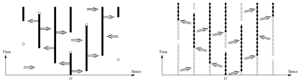
Figure 1: Graphical representation of the contact process and the discretized contact process.
2.1 Discretization
By the graphical representation, the contact process can be constructed as follows. We considerZd×R+as
space-time. Along each time line{x} ×R+, we place points according to a Poisson process with intensity 1, independently of the other time lines. For each ordered pair of distinct time lines from {x} ×R+ to
{y} ×R+, we place directed bonds ((x, t),(y, t)), t ≥ 0, according to a Poisson process with intensity
λ D(y−x), independently of the other Poisson processes. A site (x, s) is said to beconnected to (y, t) if either (x, s) = (y, t) or there is a non-zero path inZd×R
+ from (x, s) to (y, t) using the Poisson bonds and time line segments traversed in the increasing time direction without traversing the Poisson points. The law ofCt defined in Section 1.2 is equivalent to that of {x∈Zd : (o, 0) is connected to (x, t)}. See
also [22, Section I.1].
Inspired by this percolation structure in space-time and following [27], we consider an oriented perco-lation approximation in Zd×εZ
+ to the contact process, where ε∈(0,1] is a discretization parameter. We call this approximation the discretized contact process, and it is defined as follows. A directed pair
b = ((x, t),(y, t+ε)) of sites in Zd×εZ+ is called a bond. In particular, b is a temporal bond if x = y,
otherwise b is a spatial bond. Each bond is either occupied or vacant independently of the other bonds, and a bond b= ((x, t),(y, t+ε)) is occupied with probability
pε(y−x) =
(
1−ε, ifx=y,
λε D(y−x), ifx6=y, (2.1)
provided that kpεk∞ ≤1. We denote the associated probability measure by Pλ
ε. It is proved in [4] that
Pλ
ε weakly converges to Pλ as ε↓0. See Figure 2.1 for a graphical representation of the contact process
and the discretized contact process. As explained in more detail in Section 2.2, we prove our main results by proving the results first for the discretized contact process, and then taking the continuum limit when
ε↓0.
We also emphasize that the discretized contact process withε= 1 is equivalent to oriented percolation, for which λ∈[0,kDk−1
∞] is the expected number of occupation bonds per site.
We denote by (x, s) −→ (y, t) the event that (x, s) is connected to (y, t), i.e., either (x, s) = (y, t) or there is a non-zero path in Zd×εZ
+ from (x, s) to (y, t) consisting of occupied bonds. The two-point
functionis defined as
τtλ;ε(x) =Pλ
Similarly to (1.5), the discretized contact process has a critical valueλ(ε)
c satisfying
ε X
t∈εZ+ ˆ
τtλ;ε(0)
(
<∞, ifλ < λ(ε) c , =∞, ifλ≥λ(ε)c ,
lim
t↑∞P
λ
ε(Ct6=∅)
(
= 0, ifλ≤λ(ε) c ,
>0, ifλ > λ(ε)c .
(2.3)
The main result for the discretized contact process withε∈(0,1] is the following theorem:
Proposition 2.1 (Discretized results ford >4). Letd >4andδ∈(0,1∧∆∧d−24). Then, there is an
L0 =L0(d)such that, forL≥L0, there are positive and finite constantsv(ε) =v(ε)(d, L),A(ε)=A(ε)(d, L),
C1(d) and C2(d) such that
ˆ
τλ(ε)c
t;ε (√v(ε)kσ2t) =A (ε)e−|k|
2
2d £1 +O(|k|2(1 +t)−δ) +O((1 +t)−(d−4)/2)¤, (2.4) 1
ˆ
τλ(ε)c
t;ε (0)
X
x∈Zd
|x|2τλ(ε)c
t;ε (x) =v(ε)σ2t
£
1 +O((1 +t)−δ)¤
, (2.5)
C1L−d(1 +t)−d/2≤ kτλ (ε) c
t;ε k∞≤(1−ε)t/ε+C2L−d(1 +t)−d/2, (2.6)
where all error terms are uniform in ε∈ (0,1]. The error estimate in (2.4) is uniform in k ∈ Rd with |k|2/log(2 +t) sufficiently small.
Proposition 2.1 is the discrete analog of Theorem 1.1. The uniformity in ε of the error terms is crucial, as this will allow us to take the limit ε↓0 and to conclude the results in Theorem 1.1 from the corresponding statements in Proposition 2.1. In particular, Proposition 2.1 applied to oriented percolation (i.e.,ε= 1) reproves [20, Theorem 1.1].
The discretized version of Theorem 1.2 is given in the following proposition:
Proposition 2.2 (Discretized results for d≤4). Let d≤4 and δ ∈(0,1∧∆∧α). Then, there is a
λT = 1 +O(T−µ) for some µ∈(0, α−δ) such that, for sufficiently largeL1, there are positive and finite
constants C1=C1(d) and C2 =C2(d) such that, for every 0< t≤logT,
ˆ
τλT
T t;ε(√σk2 TT t
) =e−|k|
2
2d £1 +O(T−µ) +O(|k|2(1 +T t)−δ)¤, (2.7) 1
ˆ
τλT
T t;ε(0)
X
x∈Zd
|x|2τλT
T t;ε(x) =σ2TT t
£
1 +O(T−µ) +O((1 +T t)−δ)¤
, (2.8)
C1L−Td(1 +T t)−
d/2
≤ kτλT
T t;εk∞≤(1−ε)T t/ε+C2L−Td(1 +T t)−
d/2, (2.9)
where all error terms are uniform in ε∈(0,1], and the error estimate in (2.7) is uniform ink∈Rdwith |k|2/log(2 +T t) sufficiently small.
Note that Proposition 2.2 applies also to oriented percolation, for whichε= 1.
2.2 Expansion
The proof of Proposition 2.1 makes use of the lace expansion, which is an expansion for the two-point function. We postpone the derivation of the expansion to Section 3, and here we provide only a brief motivation. We also motivate why we discretize time for the contact process.
We make use of the convolution of functions, which is defined for absolutely summable functions f, g
on Zdby
(f∗g)(x) = X
y∈Zd
We first motivate the basic idea underlying the expansion, similarly as in [20, Section 2.1.1], by considering the much simpler corresponding expansion for time random walk. For continuous-time random walk making jumps fromxtoyat rateλD(y−x) with killing rate 1−λ, we have the partial differential equation
∂tqtλ(x) =λ(D∗qtλ)(x)−qλt(x), (2.11)
where qλt(x) is the probability that continuous-time random walk started at o∈Zd is at x∈Zd at time
t. By taking the Fourier transform, we obtain
∂tqˆλt(k) =−[1−λDˆ(k)] ˆqλt(k). (2.12)
In this simple case, the above equation is readily solved to yield that
ˆ
qtλ(k) =e−[1−λDˆ(k)]t. (2.13)
We see that λ= 1 is the critical value, and the central limit theorem at λ=λc= 1 follows by a Taylor expansion of 1−Dˆ(k) for small k, yielding
ˆ
qt1¡ k
√
σ2t
¢
=e−|k|
2
2d [1 +o(1)], (2.14)
where|k|2 =Pd
j=1k2i (recall also (1.1)).
The above solution is quite specific to continuous-time random walk. When we would have a more difficult function on the right-hand side of (2.12), such as−[1−λDˆ(k)] ˆqtλ−1(k), it would be much more involved to solve the above equation, even though one would expect that the central limit theorem at the critical value still holds.
A more robust proof of central limit behaviour uses induction in time t. Since time is continuous, we first discretize time. The two-point function for discretized continuous-time random walk is defined by setting q0;λε(x) =δ0,x and (recall (2.1))
qtλ;ε(x) =pε∗t/ε(x) (t∈εN). (2.15) To obtain a recursion relation for qλ
t;ε(x), we simply observe that by independence of the underlying
random walk
qλt;ε(x) = (pε∗qtλ−ε;ε)(x) (t∈εN). (2.16)
We can think of this as a simple version of the lace expansion, applied to random walk, which has no interaction.
For the discretized continuous-time random walk, we can use induction in n for all t = nε. If we can further show that the arising error terms are uniform in ε, then we can take the continuum limit ε ↓ 0 afterwards, and obtain the result for the continuous-time model. The above proof is more robust, and can for instance be used to deal with the situation where the right-hand side of (2.12) equals
−[1−λDˆ(k)]ˆqλ
t−1(k).This robustness of the proof is quite valuable when we wish to apply it to the contact process.
The identity (2.16) can be solved using the Fourier transform to give
ˆ
qtλ;ε(k) = ˆpε(k)t/ε= [1−ε+λεDˆ(k)]t/ε=e−[1−λ
ˆ
D(k)]t+O(tε[1−Dˆ(k)]2)
. (2.17)
We note that the limit of [ˆqt;ε(k)−qˆt−ε;ε(k)]/ε exists and equals (2.12). In order to obtain the central
limit theorem, we divide kby √σ2t. Then, uniformly in ε >0, we have
ˆ
q1t;ε¡ k
√
σ2t
¢
=e−|k|
2
Therefore, the central limit theorem holds uniformly inε >0.
We follow Mark Kac’s adagium: “Be wise, discretize!” for two reasons. Firstly, discretizing time allows us to obtain an expansion as in (2.11), and secondly, it allows us to analyse the arising equation. The lace expansion, which is explained in more detail below, can be used for the contact process to produce an equation of the form
∂tτˆtλ(k) =−[1−λDˆ(k)] ˆτtλ(k) +
Z t
0
ds πˆsλ(k) ˆτtλ−s(k), (2.19)
where ˆπλ
s are certain expansion coefficients. In order to derive the equation (2.19), we use that the
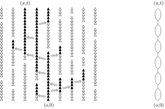
discretized contact process is oriented percolation, for which lace expansions have been derived in the lit-erature [20, 24, 25, 26, 27]. Clearly, the equation (2.19) is much more complicated than the corresponding equation for simple random walk in (2.11). Therefore, a simple solution to the equation as in (2.13) is impossible. We see no way to analyse the partial differential equation in (2.19) other than to discretize time combined with induction. It would be of interest to investigate whether (2.19) can be used directly. We next explain the expansion for the discretized contact process in more detail, following the expla-nation in [20, Section 2.1.1]. For the discretized contact process, we will regard the part of the oriented percolation cluster connecting (o,0) to (x, t) as a “string of sausages.” An example of such a cluster is shown in Figure 2. The difference between oriented percolation and random walk resides in the fact that for oriented percolation, there can be multiple paths of occupied bonds connecting (o,0) to (x, t). However, for d > 4, each of those paths passes through the same pivotal bonds, which are the essential bonds for the connection from (o,0) to (x, t). More precisely, a bond is pivotal for the connection from (o,0) to (x, t) when (o,0) −→ (x, t) in the possibly modified configuration in which the bond is made occupied, and (o,0) is not connected to (x, t) in the possibly modified configuration in which the bond is made vacant (see also Definition 3.1 below). In the strings-and-sausages picture, the strings are the pivotal bonds, and the sausages are the parts of the cluster from (o,0) in between the subsequent pivotal bonds. We expect that there are of the order t/ε pivotal bonds. For instance, the first black triangle indicates that (o,0) is connected to (o, ε), and this bond is pivotal for the connection from (o,0) to (x, t). Using this picture, we can think of the oriented percolation two-point function as a kind of random walk two-point function with a distribution describing the statistics of the sausages, taking steps in both space and time. Due to the nature of the pivotal bonds, each sausage avoids the backbone from the endpoint of that sausage to (x, t), so that any connected path between the sausages is via the pivotal bonds between these sausages. Therefore, there is a kind of repulsive interaction between the sausages. The main part of our proof shows that this interaction is weak ford >4.
Fixλ≥0. As we will prove in Section 3 below, the generalisation of (2.16) to the discretized contact process takes the form
τtλ;ε(x) =
t−ε
X•
s=0
(πλs;ε∗pε∗τtλ−s−ε;ε)(x) +πλt;ε(x) (t∈εN), (2.20)
where we use the notation P•
to denote sums over εZ+ and the coefficients πλt;ε(x) will be defined in
Section 3. In particular,πλ
t;ε(x) depends onλ, is invariant under the lattice symmetries, andπ0;λε(x) =δo,x
and πελ;ε(x) = 0. Note that for t = 0, ε, we have τ0;λε(x) = δ0,x and τελ;ε(x) = pε(x), which is consistent
with (2.20).
Together with the initial values πλ
0;ε(x) = δo,x and πλε;ε(x) = 0, the identity (2.20) gives an inductive
definition of the sequence πλt;ε(x) for t ≥ 2ε with t ∈ εZ+. However, to analyse the recursion relation (2.20), it will be crucial to have a useful representation forπtλ;ε(x), and this is provided in Section 3. Note that (2.16) is of the form (2.20) with πtλ;ε(x) =δo,xδ0,t, so that we can think of the coefficients πtλ;ε(x) for
△
Figure 2: (a) A configuration for the discretized contact process. Open triangles △ denote occupied temporal bonds that are not connected from (o,0), while closed triangles N denote occupied temporal
bonds that are connected from (o,0). The arrows denote occupied spatial bonds, which represent the spread of the infection to neighbouring sites. (b) Schematic depiction of the configuration connecting (o,0) and (x, t) as a “string of sausages.”
Our proof will be based on showing that ε12πλt;ε(x) for t≥2ε is small at λ=λ
(ε)
c ifd >4 and both t andL are large, uniformly inε >0. Based on this fact, we can rewrite the Fourier transform of (2.20) as
ˆ
fore, (2.19) is regarded as a small perturbation of (2.12) whend >4 and L≫ 1, and this will imply the central limit theorem for the critical two-point function.
Now we briefly explain the expansion coefficients πtλ;ε(x). In Section 3, we will obtain the expression
πtλ;ε(x) =
where we suppress the dependence of π(N)
t;ε(x) on λ. The idea behind the proof of (2.22) is the following.
Let
π(0)
t;ε(x) =Pελ((o,0) =⇒(x, t)) (2.23)
denote the contribution toτλ
t;ε(x) from configurations in which there are no pivotal bonds, so that
We ignore the intersection with the event that b is pivotal for (o,0) −→ (x, t), and obtain using the Markov property that
τtλ;ε(x) =π(0)
t;ε(x) + t−ε
X•
s=0
X
u,v∈Zd
π(0)
s;ε(u)pε(v−u)τt−s−ε;ε(x−v)−R(0)t;ε(x), (2.26)
where
R(0)
t;ε(x) =
X
b
Pλ ε
¡
(o,0) =⇒b, boccupied, b−→(x, t), bnot pivotal for (o,0)−→(x, t)¢
. (2.27)
We will investigate the error term R(0)t;ε(x) further, again using inclusion-exclusion, by investigating the first pivotal bond afterb to arrive at (2.22). The termπ(1)
t;ε(x) is the contribution toR
(0)
t;ε(x) where such a
pivotal does not exist. Thus, in π(0)
t;ε(x) for t ≥ε and in π
(1)
t;ε(x) for all t ≥0, there is at least one loop,
which, for Llarge, should yield a small correction only. In (2.22), the contributions from N ≥2 have at least two loops and are thus again smaller, even though allN ≥0 give essential contributions toπtλ;ε(x) in (2.22).
There are three ways to obtain the lace expansion in (2.20) for oriented percolation models. We use the expansion by Sakai [26, 27], as described in (2.23)–(2.27) above, based on inclusion-exclusion together with the Markov property for oriented percolation. For unoriented percolation, Hara and Slade [11] developed an expression for πλ
t;ε(x) in terms of sums of nested expectations, by repeated use of
inclusion-exclusion and using the independence of percolation. This expansion, and its generalizations to the higher-point functions, was used in [20] to investigate the oriented percolationr-point functions. The original expansion in [11] was for unoriented percolation, and does not make use of the Markov property. Nguyen and Yang [24, 25] derived an alternate expression for π(N)t;ε(x) by adapting the lace expansion of Brydges and Spencer [7] for weakly self-avoiding walk. In the graphical representation of the Brydges-Spencer expansion, laces arise which give the “lace expansion” its name. Even though in many of the lace expansions for percolation type models, such as oriented and unoriented percolation, no laces appear, the name has stuck for historical reasons.
It is not so hard to see that the Nguyen-Yang expansion is equivalent to the above expansion us-ing inclusion-exclusion, just as for self-avoidus-ing walks [23]. Since we find the Sakai expansion simpler, especially when dealing with the continuum limit, we prefer the Sakai expansion to the Nguyen-Yang expansion. In [20], the Hara-Slade expansion was used to obtain (2.22) with a different expression for
πt(N);ε (x). In either expansion, π(N)t;ε(x) is nonnegative for all t, x, N, and can be represented in terms of Feynman-type diagrams. The Feynman diagrams are similar for the three expansions and obey similar estimates, even though the expansion used in this paper produces the simplest diagrams.
In [20], the Nguyen-Yang expansion was also used to deal with the derivative of the lace expansion coefficients with respect to the percolation parameter p. In this paper, we use the inclusion-exclusion expansion also for the derivative of the expansion coefficients with respect to λ, rather than on two different expansions as in [20].
We now comment on the relative merits of the Sakai and the Hara-Slade expansion. Clearly, the Hara-Slade expansion is more general, as it also applies to unoriented percolation. On the other hand, the Sakai expansion is somewhat simpler to use, and the bounding diagrams on the arising Feynman diagrams are simpler. Finally, the resulting expressions for π(N)
t;ε(x) in the Sakai expansion allow for a
continuum limit, where it is not clear to us how to perform this limit using the Hara-Slade expansion coefficients.
the derivation of the lace expansion for the higher point functions, and explains the importance of the Hara-Slade expansion for oriented percolation and the contact process.
To complete this discussion, we note that an alternative route to the contact process results is via (2.19). In [5], an approach using a Banach fixed point theorem was used to prove asymptotics of the two-point function for weakly self-avoiding walk. The crucial observation is that a lace expansion equation such as (2.19) can be viewed as a fixed point equation of a certain operator on sequence spaces. By proving properties of this operator, Bolthausen and Ritzman were able to deduce properties of the fixed point sequence, and thus of the weakly self-avoiding walk two-point function. It would be interesting to investigate whether such an approach may be used on (2.19) as well.
2.3 Bounds on the lace expansion
In order to prove the statements in Proposition 2.1, we will use induction inn, wheret=nε∈εZ+. The lace expansion equation in (2.20) forms the main ingredient for this induction in time. We will explain the inductive method in more detail below. To advance the induction hypotheses, we clearly need to have certain bounds on the lace expansion coefficients. The form of those bounds will be explained now. The statement of the bounds involve the small parameter
β =L−d. (2.28)
We will use the following set of bounds:
|τˆs;ε(0)| ≤K, |∇2τˆs;ε(0)| ≤Kσ2s, kDˆ2τˆs;εk1 ≤
Kβ
(1 +s)d/2, (2.29)
where we write kfˆk1 = R[−π,π]d d dk
(2π)d|fˆ(k)| for a function ˆf : [−π, π]d 7→ C. The bounds on the lace expansion consist of the following estimates, which will be proved in Section 4.
Proposition 2.3 (Bounds on the lace expansion for d > 4). Assume (2.29) for some λ0 and all
s≤t. Then, there are β0 =β0(d, K)>0 andC =C(d, K)<∞ (both independent ofε, L) such that, for
λ≤λ0, β < β0, s∈εZ+ with2ε≤s≤t+ε, q= 0,2,4 and ∆′ ∈[0,1∧∆], and uniformly in ε∈(0,1],
X
x∈Zd
|x|q|πsλ;ε(x)| ≤ ε 2Cσqβ
(1 +s)(d−q)/2, (2.30)
¯ ¯ ¯πˆ
λ
s;ε(k)−ˆπsλ;ε(0)−
a(k)
σ2 ∇
2πˆλ s;ε(0)
¯ ¯ ¯≤
ε2Cβ a(k)1+∆′
(1 +s)(d−2)/2−∆′, (2.31)
|∂λˆπλs;ε(0)| ≤
ε2Cβ
(1 +s)(d−2)/2. (2.32)
The main content of Proposition 2.3 is that the bounds on ˆτs;ε for s≤ t in (2.29) imply bounds on
ˆ
πs;ε for all s≤t+ε. This fact allows us to use the bounds on ˆπs;ε for all arisings in (2.20) in order to
advance the appropriate induction hypotheses. Of course, in order to complete the inductive argument, we need that the induction statements imply the bounds in (2.29).
The proof of Proposition 2.3 is deferred to Section 4. Proposition 2.3 is probably false in dimensions
d ≤ 4. However, when the range increases with T as in Theorem 1.2, we are still able to obtain the necessary bounds. In the statement of the bounds, we recall thatLT is given in (1.20).
Proposition 2.4 (Bounds on the lace expansion for d≤4). Let α > 0 in (1.21). Assume (2.29), withβreplaced byβT =LT−dandσ2 byσT2, for someλ0 and alls≤t. Then, there areL0 =L0(d, K)<∞
(independent of ε) and C=C(d, K)<∞ (independent of ε, L) such that, forλ≤λ0, L1 ≥L0, s∈εZ+
with 2ε≤s≤t+ε, q= 0,2,4 and∆′ ∈[0,1∧∆], the bounds in (2.30)–(2.32) hold for t≤TlogT, with
The main point in Propositions 2.3–2.4 is the fact that we need to extract two factors of ε. One can see that such factors must be present by investigating, e.g.,π(0)t;ε(x), which is the probability that (o,0) is doubly connected to (x, t). When t > 0, there must be at least two spatial bonds, one emanating from (o,0) and one pointing into (x, t). By (2.1), these two spatial bonds give rise to two powers of ε. The proof for N ≥1 then follows by induction inN.
2.4 Implementation of the inductive method
Our analysis of (2.20) begins by taking its Fourier transform, which gives the recursion relation
ˆ (2.33). A general approach to this type of inductive analysis is given in [19]. However, here we will need the uniformity in the variable ε, and therefore we will state a version of the induction in Section 5 that is adapted to the uniformity inε and thus the continuum limit. The advancement of the induction hypotheses is deferred to Appendix A.
Moreover, we will show that the critical point is given implicitly by the equation
λ(ε)
and that the constants A(ε) and v(ε) of Proposition 2.1 are given by
A(ε) =
where we have added an argument λ(ε)
c to emphasize that λ is critical for the evaluation of πλt;ε on the
right-hand sides. Convergence of the series on the right-hand sides, ford >4, follows from Proposition 2.3. For oriented percolation, i.e., for ε= 1, these equations agree with [20, (2.11-2.13)].
The result of induction is summarized in the following proposition:
Proposition 2.5 (Induction). If Proposition 2.3 holds, then (2.29)holds fors≤t+ε. Therefore,(2.29)
holds for all s ≥ 0 and (2.30)–(2.32) hold for all s ≥ 2ε. Moreover, the statements in Proposition 2.1 follow, with the error terms uniform in ε∈(0,1].
There is also a low-dimensional version of Proposition 2.5, but we refrain from stating it.
2.5 Continuum limit
In this section we state the result necessary to complete the proof of Theorems 1.1–1.2 from Proposi-tions 2.1–2.2. In particular, from now onwards, we specialize to the contact process.
Proposition 2.6 (Continuum limit). Suppose that λ(ε) → λ and λ(ε) ≤ λ(ε)
c for ε sufficiently small.
Consequently, for λ≤λc and q = 0,2,4,
X
x∈Zd
|x|qπtλ(x)≤ Cβ (1 +t)(d−q)/2,
X
x∈Zd
∂λπtλ(x)≤
Cβ
(1 +t)(d−2)/2, (2.37)
and there exist A= 1 +O(L−d) andv = 1 +O(L−d) such that
lim
ε↓0A
(ε) =A, lim
ε↓0v
(ε) =v. (2.38)
Furthermore,∂λπλt(x) is continuous in λ.
In Proposition 2.3, the right-hand sides of (2.30)–(2.32) are proportional toε2. The main point in the proof of Proposition 2.6 is that the lace expansion coefficients, scaled byε−2, converge asε↓0, using the weak convergence of Pλ
ε toPλ [4, Proposition 2.7].
In Section 6, we will show that ε12πλt;ε(x) and ε12∂λπtλ;ε(x) both converge pointwise. We now show that
this implies that the limit of ε12∂λπλt;ε(x) equals∂λπλt(x). To see this, we use
1
ε2π
λ t;ε(x) =
Z λ
0
dλ′ 1 ε2∂λ′π
λ′
t;ε(x). (2.39)
where we use ε12π0t;ε(x) = 0 fort >0. By the assumed pointwise convergence, the left-hand side converges
toπλ
t(x), while the right-hand side converges to the integral of the limit of ε12∂λ′πtλ;′ε(x), denoted ftλ′(x) for now, using the dominated convergence theorem. Therefore, for anyλ≤λc,
πtλ(x) =
Z λ
0
dλ′ ftλ′(x), (2.40)
which indeed implies thatftλ(x) =∂λπλt(x).
Proof of Theorems 1.1–1.2 assuming Propositions 2.1–2.2 and 2.6. We only prove Theorem 1.1, since the proof of Theorem 1.2 is identical. By [4, Proposition 2.7], we have that, for every (x, t) and λ >0,
lim
ε↓0 τ
λ
t;ε(x) =τtλ(x). (2.41)
Since τλ
t(x) is continuous in λ (see e.g., [22, pp.38–39]), we also obtain limε↓0τλ (ε)
t;ε (x) = τtλ(x) for any
λ(ε) →λ. Sinceλ(ε)
c →λc[27, Section 2.1],τλ (ε) c
t;ε (x) also converges toτtλc(x). Using the uniformity inεof
the upper and lower bounds in (2.6), we obtain (1.9). Next, we prove limε↓0τˆλ
(ε) c
t;ε (k) = ˆτtλc(k) for every k ∈ [−π, π]d and t ≥ 0. Note that the Fourier
transform involves a sum over Zd, such as
ˆ
τλ(ε)c
t;ε (k) =
X
x∈Zd
τλ(ε)c
t;ε (x)eik·x. (2.42)
To use the pointwise convergence of τλ(ε)c
t;ε (x), we first show that the sum over x ∈ Zd in (2.42) can be
approximated by a finite sum. To see this, we note that
τtλ;ε(x)≤p∗εt/ε(x) =
t/ε
X
n=0
µ t/ε
n 
For any fixed t, we can choose δR ≥0, which isε-independent and decays to zero asR↑ ∞, such that
Using the above, we obtain
ˆ which proves (1.7). Similar argument can be used for (1.8).
Proof of (1.14)assuming (2.19) and Proposition 2.6. We now prove that, in the current setting, χ(λ) =
R∞
0 dtτˆtλ(0) satisfies the precise asymptotics in (1.14), assuming (2.19) and Proposition 2.6.
Let λ < λc. Since ˆτ0λ(0) = 1 and ˆτ∞λ(0) = 0, using (2.19) we obtain
By (2.34) and Proposition 2.6, λcmust satisfy
λc= 1−
Z ∞
0
ds πˆλc
s (0), (2.48)
so that we can rewrite (2.47) as
χ(λ) = [f(λc)−f(λ)]−1, (2.49)
Finally, we note that the above proof, where the integral is replaced with a sum over n ∈ Z+, also shows that the stronger version ofγ = 1 holds for oriented percolation.
3
Lace expansion
In this section, we derive the lace expansion in (2.20). The same type of recursion relation was used fordiscrete models, such as (weakly) self-avoiding walk in Zd [7, 12, 15, 19, 21, 30, 31, 32] and oriented
percolation inZd×Z+ [19, 20, 24, 25].
From now on, we will suppress the dependence on ε and λwhen no confusion can arise, and write, e.g., πt(x) = πtλ;ε(x). In Section 3.1, we obtain (3.28), which is equivalent to the recursion relation in
(2.20), and the expression (3.26) for πt(x). In Section 3.2, we obtain the expressions (3.34)–(3.35) for
∂λπt(x).
3.1 Expansion for the two-point function
In this section, we derive the expansion (3.28). We will also write Λ = Zd×εZ+, and use bold letters o,x, . . . to represent elements in Λ, such aso= (o,0) andx= (x, t), and write τ(x) =τt(x),π(N)(x) =
π(N)
t (x), and so on.
We recall that the two-point function is defined by
τ(x) =P(o−→x). (3.1)
Before starting with the expansion, we introduce some definition:
Definition 3.1. (i) For a bondb= (u,v), we write b=u and b=v. We writeb−→xfor the event
thatb is occupied and b−→x.
(ii) Given a configuration, we say that v is doubly connected to x, and we write v =⇒ x, if there are
at least two bond-disjoint paths fromv tox consisting of occupied bonds. By convention, we say
thatx=⇒xfor allx.
(iii) A bond is said to be pivotal forv−→x ifv−→x in the possibly modified configuration in which
that bond is made occupied, whereasv is not connected toxin the possibly modified configuration
in which that bond is made vacant.
We split, depending on whether there is a pivotal bond foro−→x, to obtain
τ(x) =P(o=⇒x) +
X
b
P(o=⇒b, boccupied & pivotal foro−→x). (3.2)
We denote
π(0)(
x) =P(o=⇒x), (3.3)
so that we can rewrite (3.2) as
τ(x) =π(0)(x) +
X
b
P(o=⇒b, b−→x, b pivotal foro−→x). (3.4)
Define
R(0)(
x) =
X
b
P(o=⇒b, b−→x, bnot pivotal for o−→x), (3.5)
then, by inclusion-exclusion on the event that bis pivotal foro−→x, we arrive at
τ(x) =π(0)(x) +
X
b
The evento=⇒bonly depends on bonds with time variables less than or equal to the one ofb, while the
eventb−→xonly depends on bonds with time variables larger than or equal to the one of b. Therefore,
by the Markov property, we obtain
P(o=⇒b, b−→x) =P(o=⇒b)P(boccupied)P(b−→x) =π(0)(b)p(b)τ(x−b), (3.7)
where we abuse notation to write
p(b) =p(b−b). (3.8)
Therefore, we arrive at
τ(x) =π(0)(x) + (π(0)⋆p⋆τ)(x)−R(0)(x), (3.9)
where we use “⋆” to denote convolution in Λ, i.e.,
(f⋆g)(x) =
X
y∈Λ
f(y)g(x−y). (3.10)
This completes the first step of the expansion, and we are left to investigate R(0)(
x). For this, we need
some further notation.
Definition 3.2. (i) Given a configuration andx∈Λ, we defineC(x) to be the set of sites to whichx
is connected, i.e., C(x) ={y∈Λ :x−→y}. Given a bondb, we also define ˜Cb(x) to be the set of
sites to whichxis connected in the (possibly modified) configuration in which bis made vacant.
(ii) Given a site setC, we say thatv is connected toxthrough C, if every occupied path connecting v
toxhas at least one bond with an endpoint in C. This event is written asv C
−→x. Similarly, we
write {b−→C x}={b occupied} ∩ {b C −→x}.
We then note that
{v−→b, b−→x, bnot pivotal for v−→x}=©v−→b, b
˜
Cb(v)
−−−−→xª. (3.11)
Therefore,
R(0)(
x) =
X
b
P¡
o=⇒b, b
˜
Cb(o)
−−−→x¢. (3.12)
The event{v C
−→x}can be decomposed into two cases depending on whether there is or is not a pivotal
bondb forv−→xsuch that v C
−→b. Let
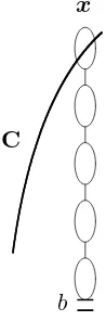
E′(v,y;C) ={v C
−→y} ∩©∄bpivotal for v−→y s.t. v C −→bª
, (3.13)
E(b,y;C) ={boccupied} ∩E′(b,y;C). (3.14)
See Figure 3 for a schematic representation of the eventE(b,x;C). If there are pivotal bonds forv−→x,
then we take the first such pivotal bondb for which v C
−→b. Therefore, we have the partition
{v C
−→x}=E′(v,x;C) ˙∪ ˙
[
b
©
E′(v, b;C)∩ {b occupied & pivotal forv−→x}ª. (3.15)
Defining
π(1) (y) =
X
b
P¡
b
x
C
Figure 3: Schematic representation of the eventE(b,x;C).
we obtain
R(0)
(x) =π(1)(x) +
X
b1,b2 P¡
{o=⇒b1} ∩E(b1, b2; ˜Cb1(o))∩ {b2 occupied & pivotal forb1 −→x}¢.
(3.17)
To the second term, we apply the inclusion-exclusion relation
{boccupied & pivotal for v−→x}={v−→b, b−→x} \©v−→b, b
˜
Cb(v)
−−−−→xª. (3.18)
We define
R(1) (x) =
X
b1,b2 P¡
{o=⇒b1} ∩E(b1, b2; ˜Cb1(o))∩©b2 ˜
Cb2(b1)
−−−−−→xª¢, (3.19)
so that we obtain
R(0)(
x) =π(1)(x) +
X
b1,b2 P¡
{o=⇒b1} ∩E(b1, b2; ˜Cb1(o))∩ {b2 −→x}¢−R(1)(x), (3.20)
where we use that
E′(v, b;C)∩ {v −→b, b−→x}=E′(v, b;C)∩ {b−→x}. (3.21)
The event{o=⇒b1} ∩E(b1, b2; ˜Cb1(o)) depends only on bonds beforeb2, while{b2 −→x}depends only
on bonds afterb2. By the Markov property, we end up with
R(0)(
x) =π(1)(x) +
X
b2
π(1)(b
2)p(b2)τ(x−b2)−R(1)(x)
=π(1)
(x) + (π(1)⋆p⋆τ)(x)−R(1)(x), (3.22)
so that
τ(x) =π(0)(x)−π(1)(x) +¡(π(0)−π(1))⋆p⋆τ¢(x) +R(1)(x). (3.23)
This completes the second step of the expansion.
To complete the expansion for τ(x), we need to investigate R(1)(x) in more detail. Note thatR(1)(x)
involves the probability of a subset of© b2
˜
Cb2(b1)
π(0)(
x) x
o
π(1)(
x) x
o
π(2)(
x) x
o
S
x
o
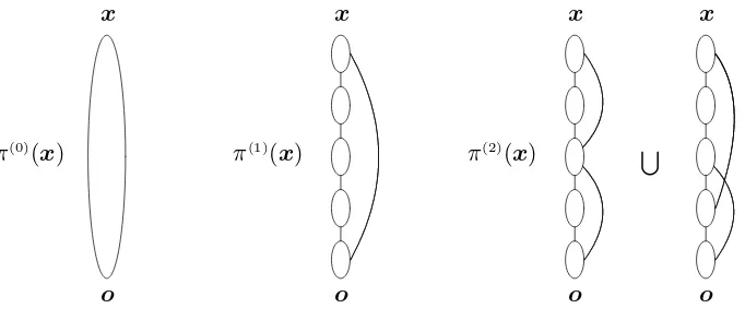
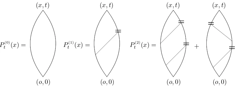
Figure 4: Schematic representations ofπ(0)(
x),π(1)(x) and π(2)(x).
For this subset, we will use (3.15) and (3.18) again, and follow the steps of the above proof. The expansion is completed by repeating the above steps indefinitely. To facilitate the statement and the proof of the expansion, we make a few more definitions. For~bN = (b1, . . . , bN) with N ≥1, we define
˜
E(N)
~bN (x) ={o=⇒b1} ∩
N−1
\
i=1
E¡
bi, bi+1; ˜Cbi(bi−1)¢∩E¡bN,x; ˜CbN(bN−1)
¢
, (3.24)
where we use the convention that b0 = o and that the empty intersection, arising when N = 1, is the whole probability space. Also, we let
˜
E(0)
~b0 (x) ={o=⇒x}. (3.25)
Using this notation, we define
π(N)(
x) =
X
~bN P¡˜
E(N)
~bN (x)
¢
, (3.26)
and denote the alternating sum by
π(x) =
∞
X
N=0
(−1)Nπ(N)(
x). (3.27)
Note that the sum in (3.27) is a finite sum, as long as tx is finite, where tx denotes the time coordinate
ofx, since each of the bondsb1, . . . , bN eats up at least one time-unitε, so thatπ(N)(x) = 0 forN ε > tx.
The result of the expansion is summarized as follows.
Proposition 3.3 (The lace expansion). For any λ≥0 andx∈Λ,
τ(x) =π(x) + (π⋆p⋆τ)(x). (3.28)
Proof. By (3.22), we are left to identifyR(1)(
x). For N ≥1, we define
R(N)(
x) =
X
~bN P¡˜
E~b(N−1)
N−1 (bN)∩
© bN
˜
CbN(bN−1)
We prove below
R(N)(
x) =π(N)(x) + (π(N)⋆p⋆τ)(x)−R(N+1)(x). (3.30)
The equation (3.28) follows by repeated use of (3.30) until the remainderR(N+1)(
x) vanishes, which must
happen at least when N ε > tx. To complete the proof of Proposition 3.3, we are left to prove (3.30),
which is a generalization of (3.22).
First we rewritebN ˜
CbN(bN−1)
−−−−−−−→xin (3.29). As in (3.15), this event can be decomposed into two cases,
depending on whether there is or is not a pivotal bond b for bN −→ x such that bN ˜
CbN(bN−1)
−−−−−−−→ b. The contribution where there is no such a bond equals E(bN,x; ˜CbN(bN−1)). If there are such pivotal bonds, then we take the first bondbamong these bonds and obtain (cf., (3.15))
© bN
˜
CbN(bN−1)
−−−−−−−→xª=E(bN,x; ˜CbN(bN−1)) ˙
∪ [˙ b
©
E(bN, b; ˜CbN(bN−1))∩ {b occupied & pivotal forbN −→x}
ª
. (3.31)
By (3.26), the contribution fromE(bN,x; ˜CbN(bN−1)) in the right-hand side isπ(N)(x), which is the first term in the right-hand side of (3.30). For the contribution from the remaining event in (3.31), we use (3.18) to arrive at
X
~bN,b P¡˜
E(N)
~bN (b)∩ {boccupied & pivotal for bN −→x}
¢
=X
~bN,b P¡˜
E(N)
~bN(b)∩ {b−→x}
¢
−R(N+1)(
x). (3.32)
The last term in the above expression is the last term in the right-hand side of (3.30). Again by the Markov property and (3.26), the first term in the right-hand side of (3.32) equals the second term in the right-hand side of (3.30). This completes the proof of (3.30) and thus the proof of Proposition 3.3.
3.2 Representation for the derivative
In this section, we derive a formula for∂λπ(x). To state the result below, we define
piv[v,x] ={b:bpivotal for v−→x}. (3.33)
Proposition 3.4. For λ >0 and x∈Λ,
∂λπ(x) = 1
λ
∞
X
N=1
(−1)NΠ(N)(
x), (3.34)
where Π(N)(
x) =PNn=1Π(N;n)(x) with
Π(N;n)(
x) =
X
~bN,b:
bspatial
P¡˜ E(N)
~bN (x)∩
©
b∈ {bn} ∪˙ piv[bn, bn+1]
ª¢
, (3.35)
and where bN+1 is defined to be x.
By the same reason as in (3.27), the sum in (3.34) is a finite sum. We prove (3.34) by differentiating the expression (3.28) forτ(x) and comparing it with the expression for∂λτ(x) obtained by using Russo’s
formula, rather than differentiating ∂λπt(x) directly. Possibly, one can also use direct differentiation of
the expressions (3.26) forπ(x), but this is cumbersome because of the complex combination ofincreasing
and decreasing events consisting of π(N)(
x), where an increasing (respectively, decreasing) event is an
Proof. In the proof it will be convenient to split
Π(N,n)(
x) = Π(N;n,1)(x) + Π(N;n,2)(x), (3.36)
where Π(N;n,1)(
x) is the contribution from b= bn in (3.35), whereas Π(N;n,2)(x) is the contribution from
b∈piv[bn, bn+1].
To obtain an expression for∂λτ(x), we useRusso’s formula [4, 9]. LetE be an increasing event that
depends only on finitely many spatial bonds. Then
∂λP(E) =
1
λ X
bspatial
P(E occurs, bis pivotal forE), (3.37)
where we use the fact that only spatial pivotal bonds for E are responsible to the differentiation with respect toλ. Let¤R= [−R, R]d∩Zd. We apply (3.37) to E=ER(x)≡ {o−→xin¤R×[0, tx]}, which
is the set of bond configurations whose restriction on bonds (u,v)⊂¤R×[0, tx] are in{o−→x}. Note
that limR→∞P(ER(x)) =τ(x), and that, for anyλ0∈[0,∞),
lim
R→∞∂λP(ER(x)) = 1
λ X
bspatial
P(o−→x, bis pivotal foro−→x), (3.38)
uniformly in λ∈[0, λ0], which we will show at the end of this section. Therefore, we can exchange the order of limR→∞ and ∂λ, and obtain
∂λτ(x) = 1
λ X
bspatial
P(o−→x, bis pivotal foro−→x). (3.39)
We follow the same strategy as in Section 3.1 to obtain a recursion relation, now for ∂λτ(x) rather
than forτ(x). Then, (3.39) equals
∂λτ(x) = 1
λ X
bspatial
·
P(o=⇒b, boccupied & pivotal for o−→x)
+X
b1<b
P(o=⇒b1, b1 and b occupied & pivotal foro−→x)
¸
, (3.40)
where P
b1<b is the sum over bonds b1 with tb1 < tb. The first and second terms in the brackets of the right-hand side correspond respectively to when b is or is not the first element of piv[o,x]. The
contribution from the first term is the same as (3.2), apart from the factor λ1 and the restriction that b
has to be a spatial bond. Thus, the first term equals
(π(0)
⋆εD⋆τ)(x) + 1
λ
∞
X
N=1
(−1)N£
Π(N;1,1)(
x) + (Π(N;1,1)⋆p⋆τ)(x)¤, (3.41)
where we abuse notation to write
D((y, s)) =D(y)δs,ε. (3.42)
For the second term in (3.40), we use
{b1 and boccupied & pivotal for o−→x}
We ignore the condition that b1 is pivotal foro−→ x and use inclusion-exclusion in the form (3.18) to
make up for the arising error. Using the Markov property, the contribution from the second term in (3.40) is
by (3.40)–(3.41) and (3.44), we have
∂λτ(x) = (π(0)⋆εD⋆τ)(x) + (π(0)⋆p⋆∂λτ)(x)−Q(1)(x)
Below, we will use inclusion-exclusion to prove that, for n≥1,
Q(n)(
Before proving (3.47), we complete the proof of (3.34) assuming (3.47). By repeated applications of (3.47) to (3.46) until the remainder termQ(n)(
x) vanishes, we obtain
∂λτ(x)−(π⋆εD⋆τ)(x) + (π⋆p⋆∂λτ)(x)
Differentiating both sides of (3.28) and comparing with the above expression, we obtain
Using this identity, we prove (3.34) by induction on tx/ε. Since π((x,0)) = δo,x and Π(N)((x,0)) = 0
for all N ≥ 1, we obtain (3.34) for tx/ε = 0. Suppose that (3.34) holds for all tx/ε ≤ m. Then the
contribution from the second term in the brackets of (3.49) equals the second term on the left-hand side of (3.49), and thus (3.34) for tx/ε=m+ 1 holds. This completes the inductive proof of (3.34).
In order to complete the proof of Proposition 3.4, we prove (3.47). Because of the conditionbn
˜
Cbn(bn−1)
−−−−−−→ xin (3.45), either the eventE(bn,x; ˜Cbn(bn−1)) occurs or there is an occupied bondbn+1 ∈piv[bn,x] for
which the eventE(bn, bn+1; ˜Cbn(bn−1)) occurs. The contribution from the former case toQ(n)(x) is
1
λ X
~bn,b:
bspatial P¡˜
E~b(n−1)
n−1(bn)∩E(bn,x; ˜C
bn(b
n−1))∩ {b∈piv[bn,x]}¢= 1
λΠ
(n;n,2)
(x). (3.50)
The contribution from the latter case is, as in (3.40),
1
λ X
~bn,b:
bspatial
·
P¡˜ E(n)
~bn(b)∩ {b occupied & pivotal forbn−→x
¢
+ X
bn+1<b P¡˜
E(n)
~bn(bn+1)∩ {bn+1 and boccupied & pivotal for bn−→x}
¢
+ X
bn+1>b P¡˜
E(n)
~bn(bn+1)∩ {band bn+1 occupied & pivotal for bn−→x}
¢ ¸
, (3.51)
where the first, second and third terms in the brackets correspond respectively to when bn+1 =b, when
bn+1 is between bn and b, and when bn+1 is between b and x. The first term is similar to that in (3.40),
and its contribution equals, as in (3.41),
(π(n)
⋆εD⋆τ)(x) + 1
λ
∞
X
N=n+1
(−1)N−n£
Π(N;n+1,1)(
x) + (Π(N;n+1,1)⋆p⋆τ)(x)¤. (3.52)
For the second term in (3.51), we apply (3.43), with b1 and obeing replaced respectively bybn+1 and
bn, and use the inclusion-exclusion relation (3.18) and the Markov property. Then, the contribution from
the second term equals, as in (3.44),
1
λ X
~bn+1,b:
bspatial P¡˜
E(n)
~bn(bn+1)∩ {bn+1 occupied & pivotal forbn−→x} ∩ {b∈piv[bn+1,x]}
¢
= 1
λ X
~bn+1,b:
bspatial P¡˜
E(n)
~bn(bn+1)∩ {bn+1 −→x} ∩ {b∈piv[bn+1,x]}
¢
−Q(n+1)(
x)
= (π(n)
⋆p⋆∂λτ)(x)−Q(n+1)(x). (3.53)
For the third term in (3.51), we use
{band bn+1 occupied & pivotal forbn−→x}
By the inclusion-exclusion relation (3.18), the contribution from the third term equals
1
λ X
~bn+1,b:
bspatial P¡˜
E~b(n)
n(bn+1)∩ {b∈piv[bn, bn+1]} ∩ {bn+1 occupied & pivotal for bn−→x}
¢
= 1
λ X
~bn+1,b:
bspatial
h
P¡˜ E~b(n)
n(bn+1)∩ {b∈piv[bn, bn+1]} ∩ {bn+1−→x}
¢
−P¡˜ E~b(n)
n(bn+1)∩ {b∈piv[bn, bn+1]} ∩ {bn+1 ˜
Cbn+1(bn)
−−−−−−→x}¢
i
, (3.55)
where the first term equals, by the Markov property,
1
λ(Π
(n;n,2)
⋆p⋆τ)(x). (3.56)
For the second term in (3.55), we use the same argument as above (3.31). Because of the condition
bn+1 ˜
Cbn+1(bn)
−−−−−−→ x, either the event E(bn+1,x; ˜Cbn+1(bn)) occurs or there is an occupied bond bn+2 ∈
piv[bn+1,x] such that E(bn+1, bn+2; ˜Cbn+1(bn)) occurs. By repeated use of inclusion-exclusion and the
Markov property, as above (3.31), the contribution from the second term in (3.55) equals
1
λ
∞
X
N=n+1
(−1)N−n£
Π(N;n,2)(
x) + (Π(N;n,2)⋆p⋆τ)(x)¤. (3.57)
Combining (3.50), (3.52)–(3.53) and (3.56)–(3.57), we obtain (3.47). This completes the proof of Proposition 3.4, assuming the uniformity of (3.38).
Proof of the uniformity of (3.38). Given λ0 ∈[0,∞), we prove that ∂λP(ER(x)) converges to the right-hand side of (3.38), uniformly inλ∈[0, λ0].
Recall thatER(x) ={o−→xin¤R×[0, tx]}. The difference between∂λP(ER(x)) and the right-hand
side of (3.38) is bounded by
1
λ
X
bspatial
b⊂¤R×[0,tx]
P¡
boccupied & pivotal for ER(x), but not pivotal for o−→x¢
+1
λ
X
bspatial
b6⊂¤R×[0,tx]
P(boccupied & pivotal for o−→x). (3.58)
First, we bound the second term, using {b occupied & pivotal for o−→x} ⊂ {o−→ b} ∩ {b−→ x} as
well as the Markov property and (2.43), by
ε X
b6⊂¤R×[0,tx]
p⋆ tb/ε(b)D(b−b)p⋆(tx−tb)/ε(x−b)≤ε
tx/ε
X
j=1
(1−ε+λε)tx/ε−j X
y∈Zd:kyk∞≥R
p∗ε(j−1)(y), (3.59)
where we take the sum over the spatial component of x to obtain the bound. Similarly to (2.44), this
is further bounded, uniformly in λ and ε, by cδ′
R where c = c(λ0, tx) and δ′R = δR′(λ0) are some finite constants satisfying limR→∞δ′R= 0.