Implementation of Evolution Strategies for
Classifier Model Optimization
Mahmud Dwi Sulistiyo
#1, Rita Rismala
#2# School of Computing, Telkom University
Jl. Telekomunikasi, Terusan Buah Batu, Bandung, Indonesia 40257
1
[email protected]
2[email protected]
Abstract
Classification becomes one of the classic problems that are often encountered in the field of artificial intelligence and data mining. The problem in classification is how to build a classifier model through training or learning process. Process in building the classifier model can be seen as an optimization problem. Therefore, optimization algorithms can be used as an alternative way to generate the classifier models. In this study, the process of learning is done by utilizing one of Evolutionary Algorithms (EAs), namely Evolution Strategies (ES). Observation and analysis conducted on several parameters that influence the ES, as well as how far the general classifier model used in this study solve the problem. The experiments and analyze results show that ES is pretty good in optimizing the linear classification model used. For Fisher’s Iris dataset, as the easiest to be classified, the test accuracy is best achieved by 94.4%; KK Selection dataset is 84%; and for SMK Major Election datasets which is the hardest to be classified reach only 49.2%.
Keywords: classification, optimization, classifier model, Evolutionary Algorithms, Evolution Strategies
Abstrak
Salah satu masalah klasik yang sering dijumpai dalam dunia kecerdasan buatan dan data mining adalah klasifikasi. Permasalahan pada klasifikasi ialah bagaimana membangun model classifier melalui proses training atau learning. Proses pembentukan model klasifikasi dapat dipandang sebagai permasalahan optimasi. Oleh karenanya, algoritma-algoritma optimasi dapat digunakan sebagai alternatif cara untuk menghasilkan model classifier tersebut. Pada penelitian ini, proses learning dilakukan dengan memanfaatkan salah satu Evolutionary Algorithms (EAs), yaitu Evolution Strategies (ES). Observasi dan analisis dilakukan terhadap beberapa parameter yang berpengaruh pada ES, serta sejauh mana model umum classifier yang digunakan pada penelitian ini. Dari percobaan dan analisis yang telah dilakukan, ES cukup baik dalam melakukan optimasi pada model klasifikasi linear yang digunakan. Untuk dataset Fisher’s Iris yang paling mudah untuk diklasifikasikan, akurasi uji terbaik yang dicapai adalah sebesar 94.4%; untuk dataset Pemilihan KK sebesar 84%; dan untuk dataset Jurusan SMK yang paling sulit untuk diklasifikasikan mencapai 49.2%.
Kata Kunci: klasifikasi, optimasi, model classifier, Evolutionary Algorithms, Evolution Strategies ISSN 2460-9056
socj.telkomuniversity.ac.id/indojc
Ind. Journal on Computing Vol. 1, Issue. 2, Sept 2016. pp. 13-26 doi:10.21108/indojc.2016.1.2.43
I. INTRODUCTION
Data classification is a classic problem often encountered in the world of artificial intelligence and data mining. In some cases, computer requires the ability of classification, as instance to recognize certain patterns, to predict a value on the specific issues of space, even to decide something or build a recommendation system.
Generally, there are two concepts in solving the problem of classification, namely memory-based and model-based classification. On the concept of memory-based, the ability to classify an input specified by the data history has ever had before. Pattern of the history data that best matches the input data is the basis to determine the class results. The concept is certainly very inflexible because it is very dependent on the availability and completeness of data. In addition, it needs large data capacity to store the history data which will be continuously increasing. Therefore, the model-based concept was commonly used instead of memory-based one.
By model-based classification, the history data is still needed, but only on the training phase, which refers to the classifier model building process. Once the training phase is completed, the history data (training data) is not needed and the system simply uses the classifier model, resulted from the training phase, to classify new input data. Various methods to train and generate the model classifier have been applied. They are like the use of Distant Supervision for Twitter sentiment classification [4], Artificial Neural Network in brain tumor detection and classification [10], as well as the use of Data Mining technique for student college enrollment approval [15]. However, a study for the optimization remains to be done since the ability of the classifier system cannot be generalized to all problems. It depends on the conditions of data involved.
Basically, the phase of training or learning is a process to produce the optimal configuration of the classifier model, given the conditions that are generally initiated at random. If it is associated with other problems in the world of artificial intelligence, the classifier model building process can be seen as an optimization problem. Therefore, optimization algorithms can also be used as an alternative way to generate a classifier model on classification problems. So far, the optimization algorithm that requires minimal cost but with optimal results in a relatively large of problem space is the optimization algorithms based on evolution concepts or commonly called as Evolutionary Algorithms (EAs). In this study, EAs will be applied as an alternative training method in the modeling classifier.
II. LITERATURE REVIEW A. Previous Works
One important step in solving the problem of classification is the process of learning which is done to build a classifier model that can map a set of attributes X to one of Y class labels that have been defined previously [7]. Classification has been widely applied in various fields, including the field of health [11, 10], education [15], social media [4, 14], and many others. If it is associated with problems in the world of artificial intelligence, the development process of this classifier models can be seen as optimization problems. In this case, the aim of optimization process is to minimize the classification error and finally obtain the classifier model.
Furthermore, a study to combine EAs and Artificial Neural Network had been conducted for time series prediction [17]. The study utilized Evolution Strategies (ES), one of EAs, to be an alternative method in the ANN training phase. The purpose was to obtain optimal weights for all neuron connections. Based on the experiments conducted, in the testing results, the error yielded by ES algorithm was tend to be better than the Back Propagation, a typical algorithm to train ANN. Therefore, the study concluded that ES algorithm was applicable as an alternative solution (substituting BP algorithm) in the learning process of the ANN. In addition, it is possible to use other prediction models [17].
B. Evolution Strategies
In this paper, one of EAs will be applied as a proposed method is Evolution Strategies.
BEGIN
5 SELECT individuals for the next generation; END
Pseudo-code 1. Evolutionary Algorithms [3]
Evolution Strategies (ES) was initially built to solve a simple parameter optimization problem. But, in the development, ES nowadays has been applied widely to deal with various problems which are more complex, like image processing and computer vision [9], scheduling [6], automatic system [13], and time series prediction [16]. The main characteristics of ES compared to other EAs can be found in the chromosome representation and the evolution operator type [2].
ES chromosome is represented as a real number which consists of three parts, namely object variable , strategy parameter of mutation step size , and strategy parameter of rotation angle . However, not all of them should be exist in an ES chromosome [3]. The chromosome representations used in this study are scheme 1 and scheme 2 which are and respectively. Note that the and symbols are used as brackets for representing chromosome contents.
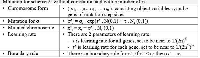
In addition, the main evolution operator used in ES is mutation [1]. The process of mutation in ES is done by adding a random number generated using normal distribution. The mutation operator is performed to whole parts of chromosome, where the mutation for should be done first before it is done for . This operator is applied for each chromosome that belongs to parent population. Basically, only successful or better resulted chromsome is kept for next generations. Technically, the process of mutation in ES depends on the chromosome scheme used. Table 1 shows mutation processes for chromosome with scheme 1 and 2 which are used in this study.
Table 1. Mutation process using scheme 1 and 2 on ES chromosome [3]
Mutation for scheme 1: without correlation and with one
Mutation for scheme 2: without correlation and with n number of
• Chromosome form • x1,…,xn, 1,…, n, consisting object variables xi and n gens of mutation step sizes
• Mutation for • ’i = i . exp(’ . N(0,1) + . Ni (0,1))
• Mutated chromosome • x’i = xi + ’i . Ni (0,1)
• Learning rate • There are 2 parameters of learning rate:
- is learning rate for all genes, set to be near to 1/(2n)½ - ’ is learning rate for each gene, set to be near to 1/(2n½)½ • Boundary rule • There is a boundary rule for ’, if ’ < 0 then ’ = 0
This unique mutation mechanism makes ES having a property of Self-adaptation, which is the ability to adapt the optimum value which probably changes all over the time by determining strategy parameters adaptively during the searching process. Along with mutation as the main operator, ES also has an addition operator namely recombination or some references call it as crossover. Recombination in ES is also applied for parent population, until gaining predetermined number of new chromosomes. The number of child chromosome targeted is influenced by a parameter called as selective pressure. Each recombination process done in ES produces only one child chromosome from two parent chromosomes.
There are two mechanisms in generating each gene for a child chromosome, namely (1) Intermediate: average value of a pair gene values of two parent chromosomes; or (2) Discrete: choosing one of two gene values from two parent chromosomes in the same index. Besides, there are two common ways as well in determining the two chromsomes as parent to produce one child chromosome, namely (1) Local: it uses only 2 chromosomes which is selected unchangedly for all child genes; or (2) Global: for every child gene, it uses different pair of parent chromsomes (generates n pairs for n child genes). As the result, there are 4 method combinations to perform recombination in ES as shown in Table 2 [18].
Table 2. Recombination methods in ES
Method One fixed pair of
chromosomes
n pairs of chromosomes for
n genes
zi = (xi + yi)/2 Local Intermediate Global Intermediate
zi = xi or yi chosen randomly Local Discrete Global Discrete
Note: z is child, while x and y are parent
Meanwhile, survivor selection is performed after gaining number of child chromosomes resulted by both mutation and recombination process of number of parent chromosomes. Generally, the survivor selection is done by selecting number of chromosomes having best fitness among others. The selecting way can be performed to 2 alternatives, namely ( + )-selection (union of parent and child chromosomes) or ( , )-selection (only child chromosomes will be involved) [18].
Overall main properties of ES can be viewed in the Table 3 below [1].
Table 3. Main properties of Evolution Strategies
Chromosome representation Real values
Parent selection Uniform distribution; using Local or Global
Mutation As main evolution operator; using Gaussian perturbation
Recombination / crossover As additional evolution operator; using Discrete or Intermediate
Survivor selection or
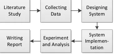
III. RESEARCH METHOD This research methodology consists of the following activities.
1. Literature study, a study of the literature related to the classification, evolutionary algorithms, as well as materials that will support this research.
2. Data collecting, a phase of collecting all the data required by the system, both for pre-research, as well as for the core of the study itself.
3. Designing the system, a stage where system is being designed, starting from the data design to analyzing the system architecture.
4. Implementation, which includes data preprocessing, feature extraction, classifier model development, and testing the system.
5. Experiment and analysis, a stage where the system is being tested to measure and analyze the system performance, including accuracy and processing time.
6. Writing report, documentation and reporting are needed for every observation and experiment results
Literature
In the Collecting Data, there are 3 kinds of data used, namely Fisher’s Iris, SMK (equal to Senior High
School) Major Election, dan Field Interest (KK) Selection dataset.
Fisher’s Iris is a dataset which is commonly used in many studies of machine learning and building
classifier model. This dataset has domain of real values and is linearly separable in term of classification, so that it is very suitable to use as a simple case study here. The total number of records in this dataset is 150, in which 100 records are for train set and the rest is for test set.
Table 4. Attribute of Fisher’s Iris dataset
Class (Species) Setosa = 1, Versicolor = 2, Virginica = 3
SMK Major Election contains students’ junior high school examination marks who will enter the SMK. Target for each input data pattern is the designated major among three options, namely Software Engineering (RPL), Multimedia, and Computer Engineering & Networks (TKJ). SMK Major Election dataset can also be used to train a classifier model for a majors recommendation system. In general, the characteristics of this dataset is non-linearly separable. Moreover, actually in determining the major, there are some subjective considerations to be involved.
This dataset consists of:
- Considering that NA is a combination value between UN and US with a particular weighting and to reduce the dimensionality of the data, the selected attribute for input is NA.
The number of records for the train set is 209, while for the test set is 90.
Table 5. Attribute of SMK Major Election dataset
Attribute (NA) Value
Indonesian Real [0 .. 10]
English Real [0 .. 10]
Math Real [0 .. 10]
Science Real [0 .. 10]
Major RPL = 1, Multimedia = 2, TKJ = 3
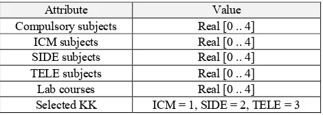
KK Selection dataset contains the courses marks taken by the students, along with the choice of each student's KK. The source of the data in this study were derived from Bachelor degree of Informatics Engineering, Telkom University. Basically, the values obtained by each student can be considered to choose which KK is suitable for him. There are 3 KKs used as the study case here: ICM (Intelligence, Computing and Multimedia), SIDE (Software Engineering, Information Systems, and Data Engineering), and TELE (Telematics). The number of records for the train set is 308, while for the test set is 131.
Indeed, not all the students always pay attention to their academic ability to determine the designated KK because there are particular personal reasons as well. However, selecting KK by students at the Telkom University also involves guardian lecturer or faculty trustee who will provide input and direction by looking at their academic potential. Therefore, the dataset for KK selection here belongs to a non-linearly separable dataset. The input of the raw data consists of marks of the courses that students have taken, that are already converted from letters into numbers. Then, those values are grouped (being averaged) into several groups of KK subjects corresponding to the course curriculum. Meanwhile the target data is the selected KK for each student having corresponding courses marks.
Table 6. Attribute of KK Selection dataset
Attribute Value
Compulsory subjects Real [0 .. 4] ICM subjects Real [0 .. 4] SIDE subjects Real [0 .. 4] TELE subjects Real [0 .. 4] Lab courses Real [0 .. 4] Selected KK ICM = 1, SIDE = 2, TELE = 3
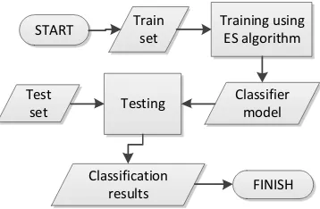
The general process flow in the system is started with input data that has been previously pre-processed. The data is the train set, which is a set of records used to build the classifier model. Next, the process goes to run training phase, the process of forming and optimizing the model, so that a classifier model is obtained. The trained model then be tested to see the performance or ability in classifying test data that had not been processed before.
Train set
Training using ES algorithm
Classifier model Test
set Testing
Classification results START
FINISH
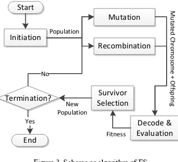
Figure 2. General overview of the classification system development using ES
The general form of the model classifier used in this study is a linear equation. Each input feature in the data is multiplied by a weight, then the product of each pair of input and weight will be totaled. The set of weight values is here said to be the classifier model. Results obtained by multiplying the number of inputs and the weights will determine the level of eligibility to be classified to a particular class. The weights given for one class are different with the weights given to other classes, but still with the same input. The output class is determined by finding the highest value among these three values of eligibility.
The purpose of the model building process here is to find the right values for all weight multipliers to be able to classify patterns of input data into classes in accordance with the best possible accuracy. Formulas (1) to (4) show the classifier models used in this study.
{
(1)
(2)
(3)
(4)
where:
: eligibility to be classified to : eligibility to be classified to : eligibility to be classified to
: input values of the data
: weights for input 1 to to get the eligibility for : weights for input 1 to to get the eligibility for : weights for input 1 to to get the eligibility for
Start
As described in the Literature Review section, here are some technical guides to perform ES algorithm.
1. Mutation process performed using the mutation step size. This explains that there is a limitation when each individual will move or mutate from the original position. Thus, the evolutionary process becomes more focused.
2. Recombination process has several choices of methods, namely Discrete or Intermediate in determining the child genes, as well as Global or Local in the parent selection process.
3. ES has a selective pressure parameter that indicates one chromosome will be compared to a number of chromosomes before being chosen as the best one and will survive in the next generation.
4. The process of recombination and mutation can be done in parallel, so the execution order is regardless.
Chromosomes that have been decoded was evaluated using the fitness formula which is defined as
In this study, a chromosome in ES represents the weighting multiplier values of each input feature data. Input values on train set are multiplied by the weights to yield the eligibility value for admission to each class, the class 1 to class n, where n is the number of classes on the data involved. By using the formula (1), the output class will be obtained for each input pattern. Fitness value is obtained by calculating the percentage level of accuracy between output and target class that has been given.
IV. RESULTS AND DISCUSSION
During the experiment, training phase through an evolution process and testing phase to see the performance of the classifier model that had been trained, was conducted using the test set. The purpose of this experiment was to analyze the influence of some parameter values on the evolutionary process and result. In addition, the observations were also done to obtain optimal combination of the parameter values, including population size, selective pressure, and recombination method.
did not change in a number of consecutive generations. Each observation was applied to 3 datasets that have been prepared, the Fisher's Iris, SMK Major Election, and KK Selection.
As the information on each resulted table to be analyzed, scheme = chromosome scheme; popOrtu = the size of the parent population; selPres = selective pressure; selOrtu = method of parent selection; hitGen = how to calculate the child's genes; accTr = average accuracy rate of train set (%); accTs = average accuracy rate of test set (%); and Wkt = average processing time (seconds).
A. Observing the Size of Parent Population
In the first stage of ES observation, there was no information related to the values of the parameters that should be used. Therefore, the determined values were commonly set. The selective pressure was 7, while the Global Discrete method was used in the recombination process.
Table 7. Observation results of the influence of parent population size to the system performance
Parameter Iris SMK Major KK Selection
Scheme popOrtu accTr accTs Wkt accTr accTs Wkt accTr accTs Wkt
1 5 79.7 78.4 0.8 60.9 49.2 1.34 71.9 69.8 2.28
1 10 88.3 82.2 2.27 61.3 47 2.72 74.8 72.3 4.49
1 20 90.7 88.6 3.52 61.5 47.4 6.6 75.8 78 9.65
1 50 95.7 92.2 11.9 61.8 47.7 17.9 75.1 74.3 21
2 5 85 83.2 0.86 60.7 48.9 1.24 66.8 66.6 1.7
2 10 92.6 87.6 2.07 61.2 46.7 2.11 70.4 69.8 4.78
2 20 97.1 92 5.36 61.2 48.2 4.5 78.8 75.8 16.1
2 50 97.9 92.4 13.3 61.4 47.2 11.8 81 77.6 42.9
The data in the table above is then simplified and resummed to obtain the average values for accuracy rate and processing time resulted by given parent population size values. Accuracy level demonstrates the ability of the model to classify the data, either on the train or test. Meanwhile, the processing time shows the speed of the ES searching process to reach convergent condition. In that condition the best-so-far solution is saturated or not changed anymore.
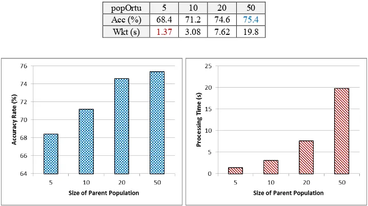
Table 8. The overall results from observation of parent population size
popOrtu 5 10 20 50
Acc (%) 68.4 71.2 74.6 75.4 Wkt (s) 1.37 3.08 7.62 19.8
Based on the overall observation results table and chart above, it appears that in terms of accuracy, the greater the parent population size are used, the ES searching process will produce a better solution models. The size of the population describes the number of chromosomes that is evaluated by ES in every generation. Among chromosomes in the population, the best chromosome is obtained for each generation. The larger the population, the greater the chance of ES to get a better solution. In this experiment, it shows that the value of 50 produces the best accuracy rate. Although this rate is still very possible to go up if the population size is increased, a value of 50 will be used as the size of the population in the next observation. It also considers that the accuracy improvement of 20 to 50 is not too high, so as expected, if the size is increased, the accuracy improvement would not be too big as well.
While in terms of processing time, it is clear that the larger the population size, the longer processing time will be taken because of more chromosomes that must be evaluated. This is certainly something to be
’paid’ if the population size is increased. The computational cost is also be considered, so it is not required to use more than 50.
B. Observation to the Selective Pressure
In the second stage of ES observation, the size of parent population used is 50, as the best result from previous observation. Meanwhile, the Global Discrete was still used as default method in the recombination process.
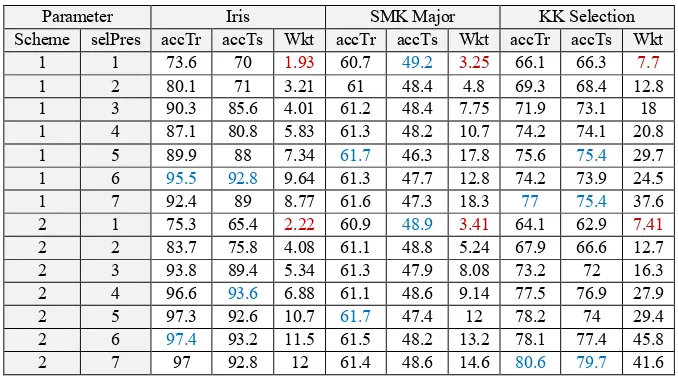
Table 9. Observation results of the influence of selective pressure to the system performance
Parameter Iris SMK Major KK Selection
Scheme selPres accTr accTs Wkt accTr accTs Wkt accTr accTs Wkt
1 1 73.6 70 1.93 60.7 49.2 3.25 66.1 66.3 7.7
1 2 80.1 71 3.21 61 48.4 4.8 69.3 68.4 12.8
1 3 90.3 85.6 4.01 61.2 48.4 7.75 71.9 73.1 18
1 4 87.1 80.8 5.83 61.3 48.2 10.7 74.2 74.1 20.8
1 5 89.9 88 7.34 61.7 46.3 17.8 75.6 75.4 29.7
1 6 95.5 92.8 9.64 61.3 47.7 12.8 74.2 73.9 24.5
1 7 92.4 89 8.77 61.6 47.3 18.3 77 75.4 37.6
2 1 75.3 65.4 2.22 60.9 48.9 3.41 64.1 62.9 7.41
2 2 83.7 75.8 4.08 61.1 48.8 5.24 67.9 66.6 12.7
2 3 93.8 89.4 5.34 61.3 47.9 8.08 73.2 72 16.3
2 4 96.6 93.6 6.88 61.1 48.6 9.14 77.5 76.9 27.9
2 5 97.3 92.6 10.7 61.7 47.4 12 78.2 74 29.4
2 6 97.4 93.2 11.5 61.5 48.2 13.2 78.1 77.4 45.8
2 7 97 92.8 12 61.4 48.6 14.6 80.6 79.7 41.6
The data in the table above is then simplified and resummed to obtain the average values for accuracy rate and processing time resulted by given selective pressure values.
Table 10. The overall results from observation of selective pressure
selPres 1 2 3 4 5 6 7
Acc (%) 64 67 72 73 74 75 75
Figure 5. Charts of the influence of the selective pressure to the ES performance for both the accuracy level and processing time
Selective pressure can describe the number of chromosomes that must be countered by a particular chromosome to be chosen as the best chromosome. For instance, if the selective pressure is set to 5, then for every group that contains (5 + 1) chromosomes taken randomly, a chromosome will be chosen as the best one to be maintained for the next generation. The amount of selective pressure on the ES will directly affect the designated number of new chromosomes that are generated through mutation and recombination operation.
Similar to previous observations, in terms of the level of accuracy that is produced, with the increasing number of new chromosomes are generated, the chance of ES to get better chromosomes is getting greater as well. ES searching process is also becoming more exploratory with more and more widespread the candidate solution is evaluated. In the first chart, it can be seen that when the value of selective pressure is increased from 1 to 6, the accuracy rates of the resulted models are continued to rise. However, when it was closed to 7, the resulted accuracy differences becomes not too far away, even almost the same. It means that the condition at that point have already started converging, so if the value of the selective pressure continues to be added, the accuracy may not be much different.
While on the other hand, the greater the value of selective pressure, the greater the computing time required. It is already quite clear since with more new chromosomes that must be evaluated, ES needs longer computational cost as well. With accuracy rates that is started to reach convergent condition, while processing time will continue to be increased, so that 7 is chosen as the optimal selective pressure in this experiment and will be used for the next observation.
C. Observation to the Recombination Method
This observation uses fixed values for several parameters obtained from previous observations. The parent population size is 50 and the selective pressure is 7. These values are used in hopes of getting the best result as well in this observation.
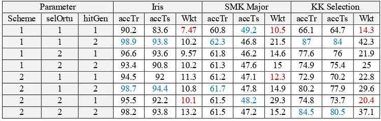
Table 11. Observation results of the influence of recombination method to the system performance
Parameter Iris SMK Major KK Selection
Scheme selOrtu hitGen accTr accTs Wkt accTr accTs Wkt accTr accTs Wkt
1 1 1 90.2 83.6 7.47 60.8 49.2 10.5 66.1 64.7 14.3
1 1 2 98.9 93.8 10.2 62.3 46.8 21.5 87 84 42.3
1 2 1 96.6 93.6 9.57 61.8 46.2 14.6 77.6 76 21.9
1 2 2 93.4 90.8 10.2 61.3 47.6 15 74.9 75.4 25
2 1 1 94.5 92 11.3 61.2 47.1 12.3 72.9 70.2 22.8
2 1 2 98.7 94.4 10.8 61.7 47.8 14.9 80.2 77.9 29.6
2 2 1 95.5 92.2 10.1 61.5 48.2 29.3 74.8 73.7 20.4
The data in the table above is then simplified and resummed to obtain the average values for accuracy rate and processing time resulted by given method combinations of parent selection and calculating child’s genes.
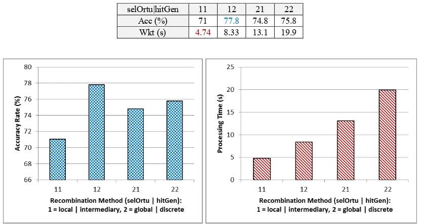
Table 12. The overall results from observation of recombination method
selOrtu|hitGen 11 12 21 22
Acc (%) 71 77.8 74.8 75.8 Wkt (s) 4.74 8.33 13.1 19.9
Figure 6. Charts of the influence of the recombination method to the ES performance for both the accuracy level and processing time
Based on the overall observation results table and chart above, it shows that the computational cost of searching process done by ES is very influenced by the recombination method used. It indicates that each recombination method has its own algorithm complexity. On the second chart, it appears that the combination of local intermediate method has the lowest complexity, while recombination with a combination of discrete global method has the highest complexity.
By selecting the parent chromosomes locally, ES only needed to find a pair of chromosomes to produce one new chromosome. While using global method, the pair of chromosomes to collect was as much as the number of genes on the chromosome. Meanwhile, the process of calculating the intermediate genes was carried only by calculating the mean between each pair of corresponding genes from both parent chromosomes. This could be done in a single process count. In contrast to the discrete method, in which for each pair of corresponding genes, ES had to choose which one would be taken for the child's gene. Thus, the process would be repeated as many times as the number of genes.
Meanwhile, calculations using discrete method (x|2) looks better than the intermediate (x|1). It can be seen from the first chart that the combination of 1|2 is better than the 1|1 and 2|2 better than 2|1. Basically, discrete method takes gene values that are already exist in the parent chromosomes. While the intermediate
method calculates parent’s genes to produce new genes with new values. So, a child generated by discrete
method is combination of values that exist in the parent chromosomes, whereas a child generated by intermediate method always has new values.
Based on the processes that occur, intermediate method tends to be faster in achieving optimum points. However, that is what makes the method getting more quickly and more likely to encounter premature convergence because it is stuck in a local optimum conditions. Meanwhile, the discrete method relatively longer to achieve optimum points. But, that feature makes ES avoids premature convergence in a local optimum point, so that the results are truly the best. In addition, based on table 7, 9, and 11, it can be seen that the results of the classification on Iris dataset is the most excellent among the three datasets were used. While the SMK Major Election dataset is the most difficult to be classified. This is caused by the Iris dataset that is linearly separable, so it will be easier to be classified by the basic model that belongs to linear classifier.
Table 13. Best accuracies of the models resulted by ES for the three datasets
Accuracy Fisher’s Iris SMK Major KK Selection
Train (%) 98.9 62.3 87
Test (%) 94.4 49.2 84
The SMK Major Election dataset that produces the lowest accuracy showed that the data pattern is the most non-linearly separable among the three datasets. It certainly makes the linear classifier model used in this study getting difficult to classify the data pattern. Thus, the low accuracy rate resulted from the experiment is not due to ES that is not capable of searching the solution, but the general classifier model that is less able to cope with the complexity of a given problem. This can be resolved by using a non-linear classification model in the next study.
V. CONCLUSION AND FUTURE WORK
Based on experiments that have been conducted, it can be concluded that ES is good enough in optimizing the linear classifier model. ES has several unique attributes and features that are beneficial in the searching process. In ES, the parameters of population size, selective pressure, and recombination method used affect the results obtained from the evolutionary process, both in terms of the accuracy rate and the processing time. Based on overall observations made, the optimal values for those three parameters are respectively 50, 7, and discrete local. For Fisher's Iris dataset, the most easily to be classified, the best testing accuracy rate achieved is 94.4%, while for KK Selection is 84%, and for SMK Major Election datasets as the hardest to reach is 49.2%. Those different results occurred by influence of the linearity of the data distribution as well as the data dimension. The more linear, the data is getting easier to be classified. Meanwhile, if the size of the data is getting bigger, commonly it is more difficult to be classified.
As for development purposes of the future works, it is necessary to use a classifier model that is more complex and can handle various conditions of data distribution, both linearly separable and non-linearly separable. In addition, it can also be compared with other methods of Evolutionary Algorithms or Swarm Intelligence based optimization method for the training phase.
ACKNOWLEDGMENT
REFERENCES
[1] Bäck, T., & Schwefel, H. P. (1993). An Overview of Evolutionary Algorithms for Parameter Optimization. Evolutionary Computation, 1(1), 1-23.
[2] Dianati, M., Song, I., & Treiber, M. (2002). An Introduction to Genetic Algorithms and Evolution Strategies. Technical report, University of Waterloo, Ontario, N2L 3G1, Canada.
[3] Eiben, A. E., & Smith, J. E. (2003). Introduction to Evolutionary Computing. Springer Science & Business Media.
[4] Go, A., Bhayani, R., & Huang, L. (2009). Twitter Sentiment Classification Using Distant Supervision. CS224N Project Report, Stanford, 1, 12.
[5] Gottlieb, J., Marchiori, E., & Rossi, C. (2002). Evolutionary Algorithms for the Satisfiability Problem. Evolutionary Computation, 10(1), 35-50.
[6] Greenwood, G. W., Gupta, A. K., & McSweeney, K. (1994, June). Scheduling Tasks in Multiprocessor Systems Using Evolutionary Strategies. In International Conference on Evolutionary Computation (pp. 345-349).
[7] Hermawati, Fajar Astuti. (2013). Data Mining. Penerbit Andi.
[8] Jones, G. (1998). Genetic and Evolutionary Algorithms. Encyclopedia of Computational Chemistry.
[9] Louchet, J. (2000). Stereo Analysis Using Individual Evolution Strategy. In Pattern Recognition, 2000. Proceedings. 15th International Conference on (Vol. 1, pp. 908-911). IEEE.
[10] Muhammad, L., Dayawati, R. N., & Rismala, R. (2014). Brain Tumor Detection and Classification In Magnetic Resonance Imaging (MRI) using Region Growing, Fuzzy Symmetric Measure, and Artificial Neural Network and Connected Component Labeling. International Journal on Information and Communication Technology| IJoICT, 1(1).
[11] Nguyen, Danh V., and David M. Rocke. "Tumor classification by partial least squares using microarray gene expression data." Bioinformatics 18.1 (2002): 39-50.
[12] Oliveto, P. S., He, J., & Yao, X. (2007, September). Evolutionary Algorithms and the Vertex Cover Problem. In Evolutionary Computation, 2007. CEC 2007. IEEE Congress on (pp. 1870-1877). IEEE.
[13] Ostertag, M., & Kiencke, U. (1995, September). Optimization of Airbag Release Algorithms Using Evolutionary Strategies. In Control Applications, 1995., Proceedings of the 4th IEEE Conference on (pp. 275-280). IEEE.
[14] Pennacchiotti, M., & Popescu, A. M. (2011). A Machine Learning Approach to Twitter User Classification. ICWSM, 11, 281-288. [15] Ragab, A. H. M., Noaman, A. Y., Al-Ghamdi, A. S., & Madbouly, A. I. (2014, June). A Comparative Analysis of Classification Algorithms for Students College Enrollment Approval Using Data Mining. In Proceedings of the 2014 Workshop on Interaction Design in Educational Environments (p. 106). ACM.
[16] Rismala, R. (2015). Prediksi Time Series Tingkat Inflasi Indonesia Menggunakan Evolution Strategies. Jurnal Ilmiah Teknologi Informasi Terapan, 1(2).
[17] Sulistiyo, Mahmud Dwi, Dayawati, R. N., Nurlasmaya. (2013, November). Evolution Strategies for Weight Optimization of Artificial Neural Network in Time Series Prediction. In Robotics, Biomimetics, and Intelligent Computational Systems (ROBIONETICS), 2013 IEEE International Conference on (pp. 143-147). IEEE.
[18] Suyanto, ST., MSc. (2008). Evolutionary Computation: Komputasi Berbasis “Evolusi” dan “Genetika”. Informatika.
![Table 1. Mutation process using scheme 1 and 2 on ES chromosome [3]](https://thumb-ap.123doks.com/thumbv2/123dok/1111025.948433/3.595.163.435.248.375/table-mutation-process-using-scheme-es-chromosome.webp)