www.elsevier.com/locate/orms
The maximum number of Hamiltonian cycles in graphs
with a xed number of vertices and edges
(
Ruud H. Teunter
a;∗, Edo S. van der Poort
baUniversity of Magdeburg, Faculty of Economics and Management, Department of Production and Logistics, P.O. Box 4120,
39016 Magdeburg, Germany
bATO-DLO, Bornsesteeg 59, 6700 AA Wageningen, The Netherlands
Received 1 May 1997; received in revised form 1 September 1999
Abstract
The problem studied in this paper is that of nding the maximum number of Hamiltonian cycles in a graph with a given number of vertices and edges. The main results are a lower bound and an upper bound, both given by closed-form closed-formulas, for the maximum number of Hamiltonian cycles in a graph with a given number of vertices and edges.
c
2000 Elsevier Science B.V. All rights reserved.
Keywords:Graphs; Theory; Traveling salesman
1. Introduction
In this paper we study the problem of determining the maximum number of Hamiltonian cycles in a graph with a given number of vertices and edges. In other words, we consider the problem of how to choose a given number of edges such that the number of Hamiltonian cycles in the resulting graph is as large as possible.
In the literature the problems involving the numbers of Hamiltonian cycles have mainly been considered for 3 and 4-regular graphs. In Tutte [10] it is shown that the number of Hamiltonian cycles in any cubic graph containing a given edge is even. Sloane [8] proves that if a graph contains two edge-disjoint Hamiltonian cycles, then there exists a third Hamiltonian cycle in this graph. Bosak [1] shows that for cubic bipartite
(When this paper was written, both authors worked at the Department of Econometrics, University of Groningen, Groningen,
The Netherlands.
∗Correspondence address: Department of Mechanical Engineering, Industrial Management Division, Aristoteles, University of Thessaloniki, P.O. Box 461, 54006 Thessaloniki, Greece.
E-mail addresses:[email protected] (R.H. Teunter), [email protected] (E.S. van der Poort)
vertices and edges. We encountered this problem, when doing sensitivity analysis on a traveling salesman problem (TSP), which is also closely related to the Hamiltonian cycle existence problem. Given a set of cities 1; : : : ; n and the distanced[i; j] between any pair of citiesi andj, the TSP is the problem of nding a shortest Hamiltonian cycle visiting each city exactly once (see e.g. Lawler et al. [4]). When studying sensitivity analysis for the TSP the following graph–theoretical problem appears to be important (see Libura et al. [5] and van der Poort et al. [7]): How many edges need to be added to a shortest Hamiltonian cycle in order to nd a set of so-called k-best cycles. A set of cycles is called k-best if the length of any Hamiltonian cycle in this set is at most the length of any Hamiltonian cycle outside the set. Clearly, in order to nd a set of
k-best Hamiltonian cycles, the number of added edges is at least the minimum number of edges that has to be added in order to obtain a graph with k Hamiltonian cycles. In other words, we are interested in the maximum number of Hamiltonian cycles in a graph with n vertices and n+a edges, for 06a6(n2)−n.
The organization of the paper is as follows. In Section 2 we mathematically formulate the problem and introduce some notations. Using brute force, exact values of the maximum number of Hamiltonian cycles in graphs with small numbers of edges are calculated in Section 3. It is also shown that the maximum number of Hamiltonian cycles in (sparse) graphs for which the number of edges is less than 1.5 times the number of vertices, only depends on the number of edges in that graph and not on the number of vertices. Lower and upper bounds of the maximum number of Hamiltonian cycles, both given by closed-form formulas and valid for any number of edges and vertices, are derived in Sections 4 and 5. We end with a comparison of the lower and upper bounds and give some conclusions and directions for future research.
2. Denitions
For n¿3, consider the complete graph Kn= (Vn; En) with the vertex set Vn={1; : : : ; n} and the edge set
En={{i; j}:i; j∈V; i6=j}. Denote mn=|En|. Any subset of En that forms a cycle containing each vertex
in Vn exactly once is called a Hamiltonian cycle in the graph Kn. Denote by Hn the set of all Hamiltonian
cycles in Kn.
For any A⊆En, the number of Hamiltonian cycles in Kn being contained in A is denoted by An, i.e.
An=|{H ∈Hn:H⊆A}|
andn(a), for a= 0;1; : : : ; mn−n, is dened as the maximum number of Hamiltonian cycles that can be found
over all sets A⊆En with|A|=n+a, i.e.
n(a) = max{An: A⊆En; |A|=n+a}:
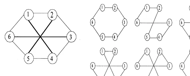
Fig. 1 shows a graph with six vertices and the corresponding set of Hamiltonian cycles for the edge set
A={{1;2}; : : : ;{5;6};{6;1};{1;4};{2;5};{3;6}}. It will be shown in Section 3 that 6(3) =A
Fig. 1. Graph with the corresponding set of Hamiltonian cycles.
LetA⊆En andU⊆Vn. Then E(A; U) denotes the set of edges in Athat are incident to two vertices in U,
i.e.
E(A; U) :={{v; w} ∈A:v; w∈U};
and, for any vertex u ∈U; Eu(A; U) denotes the set of edges in A that are incident to u and another vertex
in U, i.e.
Eu(A; U) :={{u; w} ∈A:w∈U} ⊆E(A; U):
LetA⊆En. A pathP inAis a set of adjacent edges inKn. Thelengthof a path is dened as the cardinality
of the edge set. Any pathP with end-verticesu andvis contractedinto a single edge (or vertex) when P is replaced by a single new edge{u; v}(or vertex), and all other vertices and edges in Pand all edges adjacent to ‘intermediate’ vertices of P are deleted. In the reverse operation, any single edge{u; v}can be expandedinto a path P of length k by introducing k−1 new vertices v1; : : : ; vk−1 andk edges {u; v1};{v1; v2}; : : : ;{vk−1; v}.
3. The maximum number of Hamiltonian cycles in a graph
The following lemma shows, for a given a, that forn suciently large we have that n(a) is constant.
Lemma 1. For n ¿2a it holds that n(a) =2a+1(a).
Proof. We rst show thatn+1(a)¿n(a) forn ¿2a. Let Abe such that |A|=n+a andAn=n(a). Clearly,
A contains a Hamiltonian cycle, so that every vertex is incident to at least two edges in A. There are at least n−2a ¿0 vertices that are incident to exactly two edges in A. By expanding any edge incident to one of these vertices into a path of length 2, we obtain a graph with n+ 1 vertices and the same number of Hamiltonian cycles as the original graph. Hence, n+1(a)¿n(a) for n ¿2a.
Next we show that n+1(a)6n(a) for n ¿2a−1. LetA be such that |A|=n+ 1 +a andAn+1=n+1(a). There are at least n+ 1−2a ¿0 vertices that are incident to exactly two edges in A. By contracting an edge incident to such a vertex into a single vertex we obtain a graph with n vertices and at least the same number of Hamiltonian cycles as the original graph. Hence,n(a)¿n+1(a) for n ¿2a−1. This proves that
n(a) =2a+1(a) forn ¿2a.
Unfortunately, we are not able to derive a closed-form expression for n(a). Hence, we resort to deriving
lower and upper bounds.
4. Lower bounds for n(a)
First, we prove a lemma that allows us to recursively determine a lower bound forn(a−1), given a lower
bound for n(a).
Lemma 2. Let g:=⌈2(n+a)=n⌉.For all a¿1 it holds that
n(a−1)¿
g−2
g n(a):
Proof. Let A be such that |A|=n+a and A
n =n(a). By denition of g, there is a vertex, say v, that is
incident to k¿g edges in A. Since each Hamiltonian cycle inA contains two edges incident tov, on average each of the k edges incident to v is contained in 2A
n=k Hamiltonian cycles. Hence, at least one of these k
edges, saye, is contained in at most 2A
n=k62An=g Hamiltonian cycles. So,n(a−1)¿A \{e}
n ¿An−(2=g)An=
[(g−2)=g]A
n= [(g−2)=g]n(a).
Using Lemma 2 andn(mn−n) =12(n−1)! it is possible to recursively nd lower bounds forn(mn−n);
n(mn−n−1); : : : ; n(1). Simply start with the exact lower boundn(mn−n) =12(n−1)! and, given the lower
bound for n(a), derive in each step a lower bound forn(a−1) using Lemma 2. The resulting lower bound
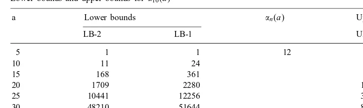
is denoted by LB-1. In Table 1 the lower bound LB-1 is given for n= 10, and several values of a. A less accurate lower bound, given by a closed-form formula, is found by replacing ⌈2(n+a)=n⌉in Lemma 2 with 2(n+a)=n, and using this same recursive argument. This leads to a lower bound LB-2 presented in Theorem 3. Lower bound LB-2 is also given in Table 1.
Theorem 3. For all a¿1 holds that
n(a)¿
1
2(n−1)!
(n+a)!
a!
(mn−n)!
mn!
:=LB-2:
Proof. The continuous function f(x) := (x − 2)=x; x ¿2, is monotonically increasing in x. Therefore, Lemma 2 gives that for all a¿1 it holds that
n(a−1)¿
⌈2(n+a)=n⌉ −2
⌈2(n+a)=n⌉ n(a)¿
(2(n+a)=n)−2 2(n+a)=n n(a) =
a
Applying this result repeatedly and using n(mn−n) =12(n−1)! gives
Similar to the derivation of the lower bounds in the previous subsection, Lemma 2 could be used to derive a recursive upper bound forn(a), that is valid for all values ofaandn. This is omitted, since a better upper
bound is derived in the remainder of this subsection. We proceed as follows. First, it is shown that n(a)
is bounded above by the solution of an integer programming problem. Then, an upper bound for n(a) is
derived by solving this integer programming problem.
Lemma 4. Let U⊆Vn; with 26|U|6n−1; and let A⊆En.Let pU be any path incident to all vertices in
Proof. The proof is by backward induction on |U|. We rst show that this lemma holds for all U with
|U|=n−1. In those casespU is a path of length n−2. Without loss of generality, let U={1;2; : : : ; n−1}
and let vertices 1 andn−1 be the endpoints of pathpU. Clearly, pU can be extended to exactly 1 Hamiltonian
cycle if the edges {1; n} and {n−1; n} are both contained in A. Otherwise, pU cannot be extended to any
Hamiltonian cycle. We show that (1) is a correct upper bound in both these cases. If the edge {n−1; n} is contained in A, then (1) gives that
max{s1:s1=|E(A;(Vn\U)∪ {u})|=|{{n−1; n}}|= 1; s161}= 1:
ways to extend any path pU, incident to all vertices in U and with endpoint u∈U, by adding an edge in
A incident to u. Clearly,|Eu(A;(Vn\U)∪ {u})|6|Vn\U|=n− |U|, since there aren− |U| vertices left to
|Eu(A;(Vn\U)∪ {u})|
ways to extend pU to a Hamiltonian cycle. In deriving the last inequality we explicitly used that |Eu(A;(Vn\
U)∪ {u})|6n− |U|. The induction step is now complete, and hence this lemma holds for allU with|U|=l.
Proof. Choose any edge from thed(u) edges inAthat are incident to vertexu. For each choice, the maximum number of possibilities for extending this edge into a Hamiltonian cycle is given by the term between brackets on the right-hand side of (2) (see Lemma 4). The factor 12 corrects for the fact that each Hamiltonian cycle is found by starting with either one of its edges incident to vertex u.
Note that the right-hand side of (2) can be considered as an integer programming problem. The solution to such a type of problem is presented in Lemma 6.
Proof. Ignoring the set of constraints si∈ {1; : : : ; i} the problem is that of maximizing a product of integers
given their sum. This is achieved by choosing these integers as close to each other as possible, since for any two integersn andm, with n ¡ m, it holds that (n+ 1)(m−1) =nm+ (m−n)−1¿mn. Hence, without the constraint si ∈ {1; : : : ; i}, the optimal solution would be either of the form {s∗1; : : : ; s∗l}={k; : : : ; k} or of the
form {s∗1; : : : ; s∗l}={k; : : : ; k; k+ 1; : : : ; k+ 1}. It is easily seen that if the set of constraints si ∈ {1; : : : ; i} is
not ignored, then the optimal solution is either of the form {s∗1; : : : ; s∗l}={1;2; : : : ; k; : : : ; k} or of the form
{s∗1; : : : ; s∗l}={1;2; : : : ; k; : : : ; k; k+ 1; : : : ; k+ 1}. The rst part {s∗1; : : : ; s∗k}={1;2; : : : ; k} is needed in order to satisfy the additional constraints. The proof is completed by noting that the largest possible value of k, is the largest value for which 1 + 2 +· · ·+k+k(l−k) =12k(k+ 1) +k(l−k)6T.
Using Corollary 5 and Lemma 6, we derive an upper bound for n(a), which is presented in Theorem 7.
Theorem 7. Let g=⌈2(n+a)=n⌉. Let k∈ {1; : : : ; n−2} be the largest integer such that y:=n+a−g−
Proof. Consider any graph with n vertices and n+a edges, and let d denote the maximum degree in this graph. Clearly, d¿g. Applying Corollary 5 and Lemma 6 gives that
n(a)6
d
2(kd+ 1)
ydkn−2−kd−yd
d kd! :=Bd; (3)
wherekd is the largest integer such that
yd:=n+a−d−12kd(kd+ 1)−kd(n−2−kd)¿0: (4)
Note that the only thing that remains to do, is proving that an upper bound forn(a) is found by replacingd
in (3) with its minimum value g. This is equivalent to showing that Bd is non-increasing in d for all d¿g,
which is done next. Combining (4) with 12kd(kd+1)+kd(n−2−kd)=(kd(kd+1)=2)+(n−2−kd)kd¿(n−2)kd=2
Table 1 gives the upper and lower bounds for n(a), derived in this paper, for graphs with 10 vertices.
Due to the recursive proof of the lower bounds, starting with a complete graph, we expect that for sparse graphs, the ratio of the upper bound and the exact value ofn(a) is much smaller than that of the exact value
and the lower bound. Unfortunately we are not able to test this hypothesis, since calculating the exact values
[5] M. Libura, E.S. van der Poort, G. Sierksma, J.A.A. van der Veen, Sensitivity analysis based on k-best solutions of the travelling salesman problem, Research Report 96A14, Graduate School=Research Institute Systems, Organizations and Management. [6] C.H. Papadimitriou, Computational Complexity, Addison-Wesley, Reading, MA, 1994.
[7] E.S. van der Poort , M. Libura, G. Sierksma, J.A.A. van der Veen, Algorithms for ndingk-best solutions of the travelling salesman problem, Research Report, Graduate School=Research Institute Systems, Organizations and Management, to appear.
[8] N.J.A. Sloane, Hamiltonian cycles in graphs of degree 4, J. Combin. Theory 6 (1969) 311–312.