www.elsevier.nlrlocatereconbase
What effect does uncertainty have on the length
of labor contracts?
Kevin J. Murphy
)Department of Economics, Oakland UniÕersity, Rochester, MI 48309, USA
Received 10 June 1998; accepted 24 June 1999
Abstract
The literature on duration of explicit labor contracts has suggested that increased uncertainty should be associated with shorter labor contracts. More recently, it has been argued that the effect of uncertainty on contract duration depends on the type of uncertainty involved. Specifically, if the uncertainty pertains to aggregate real shocks, then contract durations should increase as workers seek to insure themselves against the repercussions of such shocks. Using a sample of 1876 labor contracts signed during the period 1977–1988,
Ž
this paper provides an empirical test of the foregoing hypothesis known as the efficient risk .
sharing hypothesis . The paper presents results from estimation of a generalized-probit, simultaneous equation model, in which the dependent variables are contract length, indexation of the contract through a cost-of-living allowance, and the rate of wage change specified in the contract. The empirical findings confirm the efficient risk sharing hypothe-sis.q2000 Elsevier Science B.V. All rights reserved.
JEL classification: J50; C30
Keywords: Contract duration; Uncertainty; Efficient risk sharing
1. Introduction
The early literature on duration of explicit labor contracts suggests that increased economic uncertainty should be associated with shorter labor contracts
ŽGray, 1978 . More recent work Danziger, 1988 , however, advances the notion. Ž .
)Tel.:q1-248-370-3294; fax:q1-248-370-4275; e-mail: [email protected]
0927-5371r00r$ - see front matterq2000 Elsevier Science B.V. All rights reserved.
Ž .
that the effect of uncertainty on contract duration depends on the type of uncertainty involved. Specifically, nominal uncertainty should be associated with contracts of shorter length, but real uncertainty should be associated with contracts of greater duration.
Using a sample of 1876 labor contracts signed during the period 1977–1988, this paper tests the Danziger hypothesis. The paper specifies several measures of economic uncertainty and incorporates these in a three-equation model in which the dependent variables are contract length, the rate of wage change specified in the contract, and the propensity to index against inflation via a cost-of-living
Ž .
clause in the contract a latent variable . The model is estimated using two
Ž .
techniques described by Amemiya 1978 for estimation of a simultaneous equa-tion generalized probit model.
The remainder of the paper is structured as follows. Section 2 reviews previous theoretical and empirical work on the subject of contract duration as it relates to economic uncertainty. Section 3 presents the model of contract duration estimated in the empirical work. Section 4 relates the econometric details of estimating a simultaneous equation generalized probit model applied to the problem at hand. Section 5 discusses the empirical results. Section 6 closes the paper with a brief summary and conclusions.
2. Previous literature
The relationship of contract length and economic uncertainty was first
ad-Ž . 1
dressed in the theoretical literature in a seminal paper by Gray 1978 . Her proposition is straightforward: contract negotiation is costly for both parties; therefore, the more costly the negotiations, the longer will the length of the contract tend to be as both sides wish to spread the costs of negotiation out over time. The reason that contracts do not last forever, however, is because uncertainty vis-a-vis variables of importance to the parties to the agreement limits the length of the labor contract. In other words, contingencies such as price inflation, changes in the structure of the firm’s product market, recessions, and so forth, can occur during the life of a contract. If such events were unforeseeable when the contract was negotiated, then the real wage will deviate from that which would equate demand and supply, and losses will accumulate due to inefficient production. If an increase in the degree of uncertainty present in the economic environment occurs, then the probability that unforeseen contingencies will arise during the course of the contract increases and the negotiating parties involved will wish to sign contracts of shorter length.
1
Although the issue was not at all new to the industrial relations literature at this point in time. See,
Ž . Ž .
Ž .
Danziger 1988 develops the idea that labor contracts can insure workers against real shocks. In this light, workers are risk averse while firms are risk
Ž .
neutral or, at least, less risk averse . Over the life of a labor contract, real shocks to worker productivity can occur. Danziger argues that risk averse workers will wish to be insured against contemporaneous real shocks and will be willing to pay for such insurance by accepting lower wage growth than they would in the absence of such insurance. When the contract expires, workers are then exposed to the repercussions of the real shocks that transpired during the last contract. Danziger argues, therefore, that if a high degree of uncertainty exists regarding real shocks to the economy when a contract is negotiated, then the new contract will be commensurately longer to protect workers from the effects of such shocks. Danziger refers to this phenomenon as ‘‘efficient risk sharing’’ and he distin-guishes this from Gray’s hypothesis which he refers to as the ‘‘efficient produc-tion’’ hypothesis.
Empirical work on the general topic of contract duration is not extensive. Studies that have examined the relationship between contract duration and uncer-tainty have focussed on the nominal unceruncer-tainty distinguished by Gray rather than on the real type of uncertainty distinguished by Danziger. Most studies of the relationship between contract length and nominal uncertainty, however, do con-firm the hypothesis that this type of uncertainty and duration are inversely related.
Ž .
The first article to examine this relationship was Christofides and Wilton 1983 . Using data on Canadian contracts spanning the years 1966–1975, they found,
Ž
consistent with Gray’s hypothesis, that nominal uncertainty as measured by the
.
variance of residuals from a distributed lag estimate of inflation was associated with reduced contract length, regardless of whether wages in the contract were indexed to the rate of inflation. Employing an alternative measure of nominal
Ž .
uncertainty based on the Livingston Index of Inflation Expectations , Vroman
Ž1989 used a sample of contracts signed between 1958 and 1984 in the US.
manufacturing sector and also found that greater nominal uncertainty is associated with shorter contract length. Using a sample of Canadian contracts signed between
Ž .
1978 and 1984, Christofides 1990 estimated a three-equation model allowing for interrelationships among contract duration, rate of wage change, and the elasticity of wage indexation. Though the primary focus of his study was not on the relationship between uncertainty and contract length, he did nevertheless find some evidence to support the hypothesis of a direct link between nominal
Ž .
length. Though all of the aforementioned studies test for a relationship between nominal uncertainty and contract length, none of the studies address the point made by Danziger concerning uncertainty regarding aggregate real shocks to the economy.
3. Theoretic underpinnings
The theoretical work of Gray and later of Danziger on contract duration identify two key factors as the chief determinants of labor contract length: the cost of negotiating a labor contract and uncertainty. Negotiation costs2 are hypothesized
to be directly related to contract duration. The effect of uncertainty in the economic environment on contract length, on the other hand, depends on the type of uncertainty involved, with nominal uncertainty predicted to be associated with contracts of shorter duration and real shocks associated with longer contracts.
A third factor not addressed by Gray or Danziger that likely plays a role in determining contract length is bargaining power.3 The older, industrial relations literature on the subject does, however, emphasize the role of bargaining power in
Ž .
this context. Stieber p. 140 , for example, notes that a long term agreement ‘‘is a very substantial union concession and ‘must not be sold cheaply’’’. This follows because the union’s objective is to provide services to its constituency. One of the chief ways that a union demonstrates its usefulness is by negotiating and winning increases in compensation for the rank and file. If a long term contract is signed, then this very important channel through which the union attends to the needs of its members is lost for a period of years. This is not to say that the union will prefer a series of short contracts in order to remain continually in the bargaining process, for the union has some degree of preference for length also.4 But this
2 Ž . Ž .
Gray 1978 and Wallace and Blanco 1991 refer to these costs as ‘‘fixed costs of negotiation’’. They are fixed only in the sense that the firm would like to amortize these costs over as long a period as possible so as not to have to incur them very often. They can vary at the bargaining pair level if, for example, a strike is incurred and higher bargaining costs are borne than would have been the case had no strike taken place. Such costs also vary across bargaining unit pairs to the extent that the degree of
Ž
complexity in negotiations varies across bargaining unit pairs e.g., a contract negotiated for 50,000
.
workers will be more complex than one negotiated for 500 workers . Other authors use different
Ž .
terminology to identify the same concept. Christofides and Wilton 1983 refer to these costs as
Ž . Ž .
‘‘negotiating costs’’; Vroman 1989 refers to these costs as ‘‘contracting costs’’; and Murphy 1992 refers to the concept as ‘‘transaction costs of bargaining’’. For present purposes, the term ‘‘negotiating costs’’ seems most descriptive of the underlying concept and will be used throughout the remainder of the paper.
3 Ž . Ž .
Papers that discuss this issue at length are Hendricks and Kahn 1983 and Murphy 1992 .
4
does imply, ceteris paribus, that the union will prefer agreements of shorter duration than will the firm.
The effect of bargaining power on duration may show up both directly and indirectly. According to the argument advanced in the preceding paragraph, union bargaining power and contract length should be inversely related. The indirect channel through which bargaining power may manifest itself is via the union’s
Ž .
willingness or unwillingness to make wage concessions in return for a shorter contract. Conversely, the union may have to be compensated with larger annual wage increases than would otherwise be necessary to agree to a longer term contract. In essence, the union should need to be paid a compensating wage premium in order for it to accept a contract of greater duration.
Because of the indirect link noted in the preceding paragraph, it follows that the length of the contract and the rate of annual wage change specified in the contract are determined simultaneously in the negotiation process and, therefore, this simultaneity should be taken into account in formulating an empirical model of contract duration. In specifying the wage change equation below, I draw on previous work analyzing the wage determination process in the unionized sector. In particular, I rely on two recent papers that speak to this issue in some detail: the
Ž .
previously cited paper by Christofides and a paper by Prescott and Wilton 1992 . According to these authors, negotiated wage settlements depend on demand conditions in the labor market and on expected shifts in labor supply or labor demand during the period in which the contract will be in effect. Furthermore, if workers and firms negotiate over real wages, then the annual wage change in the
Ž
contract should also be determined by the amount of inflation both expected and
.
unexpected prevalent in the economy.
A final issue that must be addressed concerns how parties negotiating a labor agreement deal with inflation. Inflation is of concern to both labor and manage-ment since both care about real rather than nominal compensation. As noted
Ž .
above, one way to deal with inflation both anticipated and unanticipated is to negotiate contracts of short duration on a frequent basis. Frequent negotiations entail clear efficiency costs, however. Alternatively, if inflation is expected over the life of the contract, then a nominal wage change that takes such inflation into account may be negotiated directly into the contract. It will be impossible,
Ž .
however, to allow for unanticipated inflation it is unanticipated after all in this fashion. Though the costs imposed by inflation may be addressed through either or both of the aforementioned channels, both channels have clear drawbacks. It is not surprising, therefore, that unions and firms have developed a formal device — the
Ž .
cost of living allowance COLA — to mitigate the problems caused by inflation. As in the case of the rate of wage change, I draw on previous work in specifying the determination process of whether a contract contains a COLA clause. A
Ž .
seminal paper on this issue is Hendricks and Kahn 1983 , but other papers on the
Ž . Ž .
topic include Cousineau et al. 1983 , Ehrenberg et al. 1983 , Kaufman and
Ž . Ž .
more risk averse than firms. As a consequence, workers have a preference for protection from inflation and this is something they will have to ‘‘pay for’’ either by accepting a lower rate of explicit wage change or a longer contract or some combination of the two. Hence, union bargaining power should play a role in determining whether or not a contract contains an escalator clause. Additionally, the degree of uncertainty about future inflation should be positively related to the probability that a contract contains an escalator clause. If it does not appear that the price level will remain stable during the contract period, then workers will have a stronger preference for protection from inflation.
Because contract duration, the rate of wage change, and whether or not the contract contains a COLA clause are determined simultaneously in the process of negotiating a labor contract, a model that takes such endogeneity into account is appropriate. Accordingly, I report below on estimation of the following model:
DURisg D12 WAGEiqg13COLAUiqXi1b1qui1
Ž .
1DWAGEisg21DURiqg23COLAUiqXi2b2qui2
Ž .
2 COLAUisg31DURiqg D32 WAGEiqXi3b3qui3Ž .
3 where DUR is the length of contract i;i DWAGE is the annual rate of change inipay in contract i; COLAUi is the propensity for the i-th contract to be indexed by a cost of living escalator clause; COLAis1 if the i-th contract is indexed by a cost of living escalator clause and COLAis0 otherwise;gjk is the coefficient of the
Ž .
k-th endogenous variable in the j-th equation j, ks1,2,3 ; Xi j is the 1=Kj vector of exogenous regressors pertinent to the determination of the j-th endoge-nous variable; bj is the Kj=1 vector of regression coefficients corresponding to the exogenous regressors in the j-th equation; and ui j is a random disturbance term for the i-th contract in the j-th structural equation.
The vector Xi1 is of key interest since it will contain the various measures of nominal and real uncertainty as well as other proxies reflecting negotiation costs and bargaining power.
4. Econometric specification
Ž . Ž .
The system of Eqs. 1 – 3 is interesting econometrically because one of the endogenous variables, COLAU, is a latent variable and all that we actually observe
Ž .
is whether or not a contract contains an escalator clause i.e., COLAs1 or s0 . The model thus contains two continuous endogenous variables and one latent
Ž .
endogenous variable. Amemiya 1978 dubbed this the ‘‘simultaneous equation generalized probit model’’.5
5 Ž .
Before discussing estimation of this model, the use of COLAU rather than
Ž .
COLA on the right hand side of 1 warrants justification. There are two reasons to prefer use of COLAU to COLA on the right hand side of the DUR equation. First, the information included in COLAU encompasses the information in COLA. In other words, it is the desire for indexation that determines whether or not the
Ž .
contract is indexed in the first place. COLA merely reflects or ‘‘indicates’’ the level of the underlying latent variable, COLAU.6 The added benefit that one gets
by using COLAU in the model is information about other unobserved factors such as the likely degree of indexation of the contract.7 So, to use COLA when
COLAU could be used would be to discard much useful information without any additional gain. The second reason for preferring use of COLAU to COLA in the
Ž . Ž .
estimation of Eqs. 1 – 3 is that if the model were specified so that a COLA dummy were the explanatory variable in the duration equation, then the system of simultaneous equations would be rendered logically inconsistent per Heckman’s
Ž . Ž . 8
p. 936 principal assumption or logical consistency condition .
Amemiya discusses two possible ways to estimate the type of model embodied
Ž . Ž .
in Eqs. 1 – 3 . The first method yields what Amemiya refers to as the ‘‘Heckman estimator’’ while the second method yields an ostensibly more efficient, general-ized least squares estimator. I shall refer to results from this second method as the Amemiya estimator. Few applications of these estimation methods exist in the empirical literature and therefore results from both types of estimation will be reported below for comparison purposes.9,10
Estimation is carried out in two steps. In the first step, reduced form versions of
Ž . Ž .
Eqs. 1 – 3 are estimated. The reduced form parameter estimates are then used to recover the structural parameters. The reduced form equation for the j-th endoge-nous variable is:
yjsXPjqÕj
Ž .
46 Ž .
Heckman makes this point in his article p. 931 when he states that such models ‘‘ . . . rely critically on the notion that discrete endogenous variables are generated by continuous latent variables crossing thresholds.’’
7
Labor contracts that are indexed to inflation differ in the degree by which they are indexed to inflation. COLA treats all contracts with an escalator clause the same, whereas COLAU proxies directly
Ž .
for degree of indexation and risk aversion .
8
I provide a proof of this proposition in an unpublished appendix that is available on request. In essence, the issue is that one would need to assume that the dummy variable is exogenous in order for the model to be logically consistent, which is counter to the notion that contract length, indexation, and rate of wage change are determined simultaneously in the process of contract negotiation.
9 Ž .
Two papers which do apply these estimation methods are Thomas et al. 1991 and DeBrock et al.
Ž1996 .. 10
where P is the K=1 vector of reduced-form regression coefficients; and Õ is a
j j
random disturbance term.
Ž .
Eq. 4 can be estimated by ordinary least squares for DUR and DWAGE. Because COLAU is only observed dichotomously, however, the reduced-form equation in the case of this variable is estimated via maximum likelihood estimation applied to a probit model of COLAU.
Ž . Ž .
In order to estimate the structural parameters in Eqs. 1 – 3 , the reduced form equation estimates must be substituted in an appropriate fashion back into Eqs.
Ž . Ž .1 – 3 . Thus:
ˆ
ˆ
DURsg12XP2qg13XP3qX1b1
ˆ
ˆ
q Õ1yg12X
Ž
P2yP2.
yg13XŽ
P3yP3.
ˆ
XsXH1a1qw1
Ž .
1ˆ
Žˆ
ˆ
.where H1s P2,P3, J ; J is a K1 1 =K1 matrix of zeros and ones such that
w xX Ž .
XJ1sX ;1 a1s g12,g13,b1 and is a K1q2 =1 vector of regression coeffi-cients; and w is a random disturbance vector.11
1
In order to obtain the Heckman estimator of the vector of structural parameters for the first equation, a1 is estimated via least squares by taking:
y1
X X X X
ˆ
ˆ
ˆ
a
ˆ
1sž
H X XH1 1/
H X DUR.1Ž .
5 aˆ
1’s variance is given by:y1 y1
X X X X X X
ˆ
ˆ
ˆ
ˆ
ˆ
ˆ
Var
Ž
aˆ
1.
sž
H X XH1 1/
Ž
H X Var w1Ž
ˆ
1.
XH1.
ž
H X XH1 1/
.Ž .
6Amemiya proposed a more efficient generalized least squares procedure for estimation of a1, however. Amemiya’s GLS estimator is obtained by taking:
y1
y1 y1
X X
G
ˆ
ˆ
ˆ
ˆ
a
ˆ
1sž
H Var1Ž
hˆ
1.
H1/
H Var1Ž
hˆ
1.
P1Ž .
7whereh is a disturbance term.The variance of a
ˆ
G is given by:1 1
y1
y1 X
G
ˆ
ˆ
Var
Ž
aˆ
1.
sž
H Var1Ž
hˆ
1.
H1/
.Ž .
8Ž .
Estimation of Eq. 2 proceeds, with appropriate substitutions, similar to Eq.
Ž .X U
1 . The COLA equation must be treated differently than the duration equation
Ž .
and the wage change equation, however. The left hand side of Eq. 3 is, econometrically speaking, unobservable. That is, the econometrician knows when
11
Notice thatÕ, the reduced form disturbance, rather than u is a component of w . u drops out of
1 1 1 1
the equation when the reduced form estimators for the other two endogenous variables are substituted
Ž .
the desire to index is strong enough to result in an indexation clause; however, the
Ž .
desire to index, which is what is on the left hand side of Eq. 3 , is unobservable.
U Ž .
Substituting the reduced form equation for COLA sXŁ qÕ on the left
3 3
Ž .
hand side of Eq. 3 , yields:
XP3qÕ3sg31DURqg D32 WAGEqX3b3qu .3
Ž .
3XSolving for the observable DUR results in:
ˆ
ˆ
DURs
Ž
1rg31.
XP3yŽ
g32rg31.
XP2yŽ
1rg31.
X3b3ˆ
ˆ
q Õ1y
Ž
g32rg31.
XŽ
P2IP2.
yŽ
1rg31.
XŽ
P3IP3.
ˆ
YsXQlqw3
Ž .
3where
ˆ
ˆ
ˆ
Qs P3,IP2,yJ3 ;
w
J is a K3 =K3 matrix of zeroes and ones such that XJ3sX ; and3 ls 1rg31,
Ž . xX
g32rg31, 1rg31 b3 .
Ž .
Amemiya shows that the Heckman estimator of l via least squares is:
y1
X X X X
ˆ
ˆ
ˆ
ˆ
ls
Ž
Q X XQ.
Q X DUR.Ž .
9ˆ
The parameter estimates of interest — g
ˆ
31,gˆ
32,b3— can easily be identified fromˆ
Ž .l. The variance–covariance matrix for g31,g32, b3 can also be estimated using
ˆ
the variance–covariance matrix of l.
As was true of the parameter estimates for DUR and DWAGE, Amemiya’s paper proposes a more efficient GLS estimate for the parameter vector
correspond-ˆ
wˆ
ˆ
xing to the latent variable. This is obtained by forming Gs P1,P2,J3 and then
Ž Ž ..
calculating the estimate of the parameter vectora3 s g31,g32, b3 such that:
y1
y1 y1
X X
G
ˆ
ˆ
ˆ
ˆ
a
ˆ
3sž
G VarŽ
hˆ
3.
G/
G VarŽ
hˆ
3.
P3Ž
10.
where h is a disturbance term.The variance–covariance matrix of aG is
ˆ
3 3
obtained by taking:
y1
y1 X
G
ˆ
ˆ
Var
Ž
aˆ
3.
sž
G VarŽ
hˆ
3.
G/
.Ž
11.
5. Data and empirical results
Ž . Ž .
The contract data used in estimating Eqs. 1 – 3 were drawn from Current
Ž .
sample consists of 1876 contracts negotiated between 1977 and 1988 covering
Ž .
firm-union bargaining pairs in a variety of industries spanning all broad 1-digit sectors of the economy. Mean contract length during the sample period is 29.5 months. The standard deviation and the range of the data are 9.4 months and 4.6 years, respectively.
5.1. Uncertainty measures
Since the focus of this paper is on the effect of uncertainty on contract duration, it is worth discussing the definitions of the uncertainty variables in some detail at the very outset. In his theoretical work, Danziger showed that three types of uncertainty should be important in determining contract length: nominal uncer-tainty, relative unceruncer-tainty, and real uncertainty. The empirical question is how to measure each concept.
Nominal uncertainty is the easiest to measure in the sense that previous contract duration studies employ measures of this type of uncertainty in their analyses. The variable measuring nominal uncertainty in the empirical work below is entitled INFUNCRT. It was constructed using the sliding regression technique advocated by Christofides and by Christofides and Wilton. Specifically, the inflation rate was regressed against past values of itself in an 11-lag, third-degree polynomial. The sample period begins in the third quarter of 1959 and extends to the quarter prior to signing of a given contract. Thus 44 regressions were run in all. The inflation
Ž .
data specifically, the percent change in the GNP deflator were drawn from the CITIBASE database. The nominal uncertainty measure is the mean square error of the regression pertaining to the relevant year and quarter prior to signing of the contract of interest.12 This method presumes that agents are able to forecast
inflation on the basis of the past behavior of inflation and that they have no more information available to them than is available at the time of the contract negotiations.
In his QJE paper, Danziger also argued that ‘‘relative’’ uncertainty would be inversely related to contract length. In this regard, he was referring to uncertainty
Ž .
of consumer prices i.e., prices that matter to consumers vis-a-vis producer prices
Ži.e., prices that matter to firms . The variable used in the empirical work to.
measure this aspect of uncertainty is RELUNCRT. It is constructed in a fashion similar to INFUNCRT using the sliding regression technique. Specifically, the ratio of the consumer price index to the producer price index was regressed against past values of this ratio using an 11-lag, third degree polynomial.13 The mean
12
In other words, if the contract of interest was signed in June of 1985, then the mean square error of the regression spanning the period 59III–85I was used as the measure of nominal uncertainty.
13 Ž .
square error of this regression up to the quarter before the signing of the contract was used as the uncertainty measure.
The measure of chief interest to this study is that which proxies for what Danziger referred to as real uncertainty. The literature is not very specific about exactly what constitutes a real shock. Real shocks may be due to an unexpected
Ž .
price change for some crucial input in the production process e.g., oil . A real shock may occur because of an unexpected change in productivity or technology.
Ž
Or such a shock may occur because of a change in preferences say, consumer
.
demand or labor supply . All of these factors are difficult to measure, but changes in such factors should affect the aggregate unemployment rate. In order to measure real uncertainty, therefore, I applied the sliding regression technique to the aggregate unemployment rate. Specifically, the following regression was fit for the quarterly aggregate unemployment rate:
usdq bu q g p q
Ž
1yu Byu B2.
´Ž
12.
Ý
Ý
t i tyi i tyi 1 2 t
i i
where u is the aggregate unemployment rate at time t;t p is the rate of inflation; and B is the backward shift operator.
After some experimentation, it was determined that the lagged unemployment rate terms were best treated as an 11-lag, third-degree polynomial, while the lagged inflation terms were best treated as an 11-lag, second degree polynomial. Lagged inflation is included in the regression in order to purge the effect of excess demand from the unemployment rate. The unemployment rate data commence in 1960 and a regression was run from 1960 to the quarter in which the contract of interest was signed. The real uncertainty measure is the mean square error of this regression and is referred to as URUNCERT in the work below.
This measure of real uncertainty is related to changes in the unemployment rate that can neither be predicted from past movements in the rate of inflation nor from past movements in the rate of unemployment. By allowing for the rate of inflation
Ž
in the regression, changes in unemployment due to nominal factors such as
.
changes in the money supply or changes in fiscal policy are accounted for. As an additional control for real uncertainty, I also created a variable measuring
Ž .
real uncertainty within the local labor market RLURSDLG . In order to generate this variable, state unemployment was first predicted by regressing the state unemployment rate against the lagged state unemployment rate, against the national and the lagged national unemployment rate, and against a cubic function of time. The time period for the regression is 1960 to the year prior to the contract
Žthus, the presumption is that agents only have information to the present ..
5.2. Additional exogenousÕariables
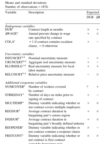
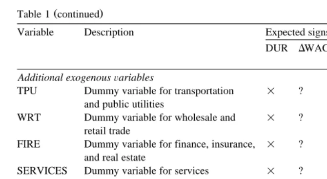
A number of other variables were used as proxies for the factors sketched as determinants of DUR, DWAGE, and COLAU in Section 3. Table 1 provides definitions and summary statistics, indicates whether a given variable was included
Ž . Ž .
in the X matrices of Eqs. 1 – 3 , and indicates the expected signs of the includedj variables in a given X matrix.j
NUMCOVER is the number of employees covered by the contract. It serves as a proxy both for negotiation costs, in that a larger bargaining unit implies that a more complex contract must be negotiated, and for union bargaining power, in that more workers can impose heavier strike costs on firms. It cannot be signed in the DUR equation since negotiation costs and union bargaining power are hypothe-sized to have opposing effects on duration. It should have a positive impact on both DWAGE and COLAU, however, since negotiation costs do not affect either variable and since greater union bargaining power should imply that a given union is able to win a larger wage increase and able to secure better protection against inflation.
STRKEDAY is the number of days on strike leading up to an agreement. This variable, like NUMCOVER, proxies both negotiation costs and union bargaining power. One can surmise from mean strike length given in Table 1 that most contracts are negotiated without ever incurring a strike. To the extent strikes do occur, however, it is assumed that longer strikes are associated with higher negotiation costs and that longer strikes are inversely related to union bargaining power.14 It is expected then that contract duration and strike length will be
positively related since a long strike implies both high cost of negotiation and low union bargaining power. It is also expected that strike length will be inversely related toDWAGE and COLAU since a longer strike implies less union bargaining power.
MULTIEMP is a dummy variable for whether or not the contract covers multiple employers. This variable should be directly related to negotiation costs, since negotiating a contract to cover multiple employers entails more complex negotiations, and should be inversely related to union bargaining power, since organization of employers implies greater firm bargaining power, other things being equal. It is hypothesized that the variable has a positive impact on contract duration and a negative impact on the likelihood that a cost of living clause is incorporated in the contract.
REGDUR and INDDUR are, respectively, the average contract duration in the
Ž .
relevant region Northeast, North Central, South, or West and in the relevant,
Ž .
broadly defined industry manufacturing, non-manufacturing, or public sector in
14
the quarter in which the contract is signed. These variables are included to control for the possibility that firm-union bargaining pairs emulate other bargaining pairs in their region or in their industry, thus both variables are expected to be positively related to contract duration.15
REOPENER is a dummy variable for whether or not the contract contains a reopener clause. Contract reopeners act as another means by which bargaining pairs deal with uncertainty. That is, if unexpected inflation occurs over the life of the contract, then the contract can be reopened to adjust the wage appropriately. Thus it is expected this variable will be negatively related to the rate of wage change and that the probability that the contract will contain a cost of living adjustment clause will be lower since the reopener serves much the same purpose as the COLA clause.
LVEXPINF is the expected rate of inflation from the Livingston index of inflation expectations for the period in which the contract is signed. Because workers care about real compensation, this variable should be positively related to the annual rate of wage change negotiated in the contract. It should, moreover, be positively related to the likelihood that the contract contains a COLA clause since expected inflation and unexpected inflation are likely to be positively correlated. UDIFFLAG is included as a proxy for excess demand conditions. It is the state unemployment rate minus the state natural rate of unemployment in the year before the contract is signed.16 The larger is this variable the weaker is the economy in the state in which the agreement is signed; therefore, it is expected thatDWAGE will be inversely related to this variable and also that it will be less likely that the contract will contain a COLA clause.
Ž
PDOT and PDOTLAG are the annualized quarterly inflation rates based on the
.
GNP deflator in the quarter in which the contract was signed and in the immediately preceding quarter. These variables reflect current and past inflation but also may serve as proxies for expected future inflation; therefore, both variables enter the DWAGE and COLAU equations with positive signs.
AFLCIO is a dummy variable for whether or not the union is affiliated with the AFL-CIO. The maintained hypothesis is that unions affiliated with the AFL-CIO have greater bargaining power. Thus one would expect that affiliated unions will have a greater likelihood of securing a cost of living clause in a contract than will non-affiliated unions.
15
An anonymous referee points out, however, such positive association could also result if REGDUR and INDDUR proxy for unmeasured variables in the region or industry that all bargaining pairs, including the bargaining pair of interest, are responding to.
16
Table 1
Means and standard deviations Number of observationss1876.
Variable Description Expected signs Mean
U Žstandard DUR DWAGE COLA
.
deviation
EndogenousÕariables
a Ž .
DUR Contract length in months = q q 29.55 9.40
a Ž .
DWAGE Annual percent change in wage q = q 3.65 2.81
rate specified by contract
a Ž .
COLA s1 if contract contains escalator q y = 0.171 0.377
clause,s0 otherwise
UncertaintyÕariables
b,d Ž .
INFUNCRT Nominal uncertainty measure y q q 2.688 0.104
b,d Ž .
URUNCERT Aggregate real uncertainty measure q y = 9.232 0.906
c,d Ž .
RLURSDLG Real uncertainty measure for local q q = 0.755 6.846 labor market
b,d Ž .
RELUNCRT Relative price uncertainty measure y = y 9.904 0.219
Additional exogenousÕariables
a
NUMCOVER Number of workers covered ? q q 4482.99
Ž .
by contract 16408.61
a Ž .
STRKEDAY Number of days on strike prior to q y y 2.57 19.08
signing of contract
a Ž .
MULTIEMP Dummy variable indicating whether or q = y 0.077 0.267 not contract covers multiple employers
d Ž .
REGDUR Average contract duration in q = = 29.79 2.856
bargaining pair’s census region
d Ž .
INDDUR Average contract duration in q = = 29.62 3.353
bargaining pair’s broadly defined industry
a Ž .
REOPENER Dummy variable indicating whether or = y y 0.102 0.302 not contract contains a reopener clause
a Ž .
FRSTCONT Dummy variable indicating whether or = = y 0.213 0.410 not contract is first contract
signed by bargaining pair
a,e Ž .
AFLCIO Dummy variable indicating whether or = = q 0.74 0.439 not union is affiliated with AFL-CIO
b Ž .
LVEXPINF Expected rate of inflation for period in = q q 4.692 1.045 which the contract was signed
c,d Ž .
UDIFFLAG State unemployment rate minus = y y 0.237 1.081
state natural rate of unemployment
b Ž .
PDOT Annualized inflation rate for quarter in = q q 3.695 1.924 which contract is signed
b Ž .
PDOTLAG Annualized inflation rate for quarter = q q 3.671 1.604 prior to signing of contract
Ž .
NONDRMFG Dummy variable for non-durable = ? ? 0.125 0.331
manufacturing
Ž .
MINING Dummy variable for mining = ? ? 0.002 0.046
Ž .
Ž .
Table 1 continued
Variable Description Expected signs Mean
U Žstandard DUR DWAGE COLA
.
deviation
Additional exogenousÕariables
Ž .
TPU Dummy variable for transportation = ? ? 0.146 0.353
and public utilities
Ž .
WRT Dummy variable for wholesale and = ? ? 0.027 0.163
retail trade
Ž .
FIRE Dummy variable for finance, insurance, = ? ? 0.0064 0.080 and real estate
Ž .
SERVICES Dummy variable for services = ? ? 0.283 0.451
Ž .
PUBADMIN Dummy variable for public = ? ? 0.223 0.416
administration
Ž .
NRTHEAST Dummy variable for northeast region = ? ? 0.235 0.424
Ž .
MIDWEST Dummy variable for midwest region = ? ? 0.237 0.425
Ž .
SOUTH Dummy variable for south region = ? ? 0.183 0.387
Ž .
WEST Dummy variable for west region = ? ? 0.216 0.412
a
Current wage developments.
b
CITIBASE database.
c
Statistical Abstract of the United States, various issues.
d
Tabulation by author.
e
Directory of National Unions and Employee Associations.
Dummy variables for one-digit industries and for the major census regions are also included to serve as additional control variables in the auxiliaryDWAGE and COLAU equations. The base industry is durable manufacturing and the base region
Ž
is the national level i.e., most contracts cover workers in a given region, but about
.
13% of contracts cover workers at the national level .
5.3. Empirical results
Ž . Ž .
Table 2
Ž .
Regression results t-statistics are in parentheses
U
Ž . Ž . Ž .
Variables 1 DUR 2 DWAGE 3 COLA
Heckman Amemiya Heckman Amemiya Heckman Amemiya
Endogenous
DURATION – – y0.018 y0.021 0.059 0.055
Žy0.39. Žy0.47. Ž2.95. Ž2.82.
DWAGE y0.454 y0.446 – – y0.414 y0.431
Žy2.31. Žy2.26. Žy1.28. Žy1.33.
COLA 0.399 0.411 0.678 0.702 – –
Ž1.19. Ž1.22. Ž0.92. Ž0.95. Exogenous
CONSTANT 34.245 34.272 y5.214 y5.136 y13.848 y14.179
Ž2.32. Ž2.32. Žy1.92. Žy1.89. Žy1.80. Žy1.85.
NUM-COVER 0.0164 0.0162 y0.00436 y0.00472 0.0108 0.011
Žin thousands. Ž1.34. Ž1.33. Žy0.50. Žy0.54. Ž2.13. Ž2.17.
STRKEDAY 0.019 0.019 y0.007 y0.007 y0.004 y0.004
Ž1.92. Ž1.92. Žy2.07. Žy2.06. Žy1.31. Žy1.32.
MULTIEMP 0.021 0.031 – – 0.007 0.020
Ž0.03. Ž0.04. Ž0.04. Ž0.09.
REGDUR 0.923 0.923 – – – –
Ž12.30. Ž12.29.
INDDUR 0.683 0.683 – – – –
Ž8.12. Ž8.11.
INFUNCRT y5.002 y5.018 3.987 4.033 0.643 0.669
Žy2.03. Žy2.04. Ž2.11. Ž2.13. Ž0.79. Ž0.82.
RLURSDLG y0.015 y0.015 0.019 0.019 – –
Žy0.52. Žy0.53. Ž1.66. Ž1.66.
URUNCERT 0.544 0.548 y0.531 y0.539 – –
Ž2.23. Ž2.24. Žy1.86. Žy1.89.
RELUNCRT y4.234 y4.234 – – 1.004 1.045
Žy3.93. Žy3.93. Ž1.84. Ž1.92.
REOPENER – – y1.213 y1.184 y1.359 y1.351
Žy2.10. Žy2.05. Žy2.46. Žy2.45.
FRSTCONT – – – – 0.001 0.017
Ž0.01. Ž0.10.
AFLCIO – – – – 0.088 0.094
Ž0.50. Ž0.54.
LVEXPINF – – 0.354 0.355 0.172 0.186
Ž2.02. Ž2.03. Ž0.77. Ž0.83.
UDIFFLAG – – y0.107 y0.108 0.063 0.064
Žy1.09. Žy1.10. Ž1.11. Ž1.13.
PDOT – – y0.038 y0.040 0.026 0.026
Žy0.37. Žy0.40. Ž0.60. Ž0.58.
PDOTLAG – – y0.088 y0.092 0.069 0.064
Žy0.81. Žy0.84. Ž1.41. Ž1.32.
NRTHEAST – – 2.031 2.046 0.090 0.130
Ž .
Table 2 continued
U
Ž . Ž . Ž .
Variables 1 DUR 2 DWAGE 3 COLA
Heckman Amemiya Heckman Amemiya Heckman Amemiya
Exogenous
MIDWEST – – 1.460 1.468 0.206 0.225
Ž4.17. Ž4.19. Ž0.50. Ž0.55.
SOUTH – – 1.514 1.517 0.257 0.267
Ž4.28. Ž4.29. Ž0.58. Ž0.61.
WEST – – 1.219 1.225 0.279 0.287
Ž3.92. Ž3.94. Ž0.73. Ž0.75.
MINING – – 0.095 0.096 y0.444 y0.490
Ž0.07. Ž0.07. Žy0.52. Žy0.57.
CONSTRUC – – y1.772 y1.772 y1.907 y1.990
Žy2.40. Žy2.40. Žy2.12. Žy2.22.
NONDRMFG – – 1.559 1.584 y0.912 y0.913
Ž1.73. Ž1.76. Žy3.59. Žy3.59.
TPU – – 1.758 1.766 y0.179 y0.182
Ž3.00. Ž3.02. Žy0.45. Žy0.45.
WRT – – 0.766 0.807 y1.695 y1.695
Ž0.63. Ž0.67. Žy5.52. Žy5.52.
FIRE – – 1.426 1.435 y0.233 y0.245
Ž1.48. Ž1.49. Žy0.40. Žy0.42.
SERVICES – – 3.651 3.677 y0.752 y0.760
Ž2.67. Ž2.69. Žy0.95. Žy0.96.
PUBADMIN – – 2.880 2.912 y1.020 y1.033
Ž2.15. Ž2.18. Žy1.86. Žy1.88. 2
R 0.205 0.205 0.198 0.198 – –
Finally, the R2s in the equations for the continuous variables exhibit no apparent change whatsoever by technique.17
Because the focus of this study is contract duration, I shall proceed by first
Ž .
discussing in detail the regression results for Eq. 1 and then conclude with a briefer discussion of the results for the wage change equation and the indexation
Ž .
equation. Of the two right-hand-side endogenous variables in Eq. 1 , only the rate of wage change has a significant impact on contract duration. Contracts specifying
Ž
higher rates of annual wage change tend to be somewhat shorter in length the
.
implied elasticity is small, however, aty0.055 . The indexation variable has the expected sign but is not statistically significant.
Of the exogenous variables not related to economic uncertainty, the average
Ž . Ž .
contract duration found in the region REGDUR and in the industry INDDUR exert the strongest influence on the length of contract signed by a bargaining pair.
17
A one month increase in average duration in the region is associated with nearly a one month increase in bargaining pair specific contract length, while at the industry level an extra month is associated with more than an additional half of a month of duration. These results suggest that bargaining pairs tend to emulate other bargaining pairs in the relevant region and industry. Table 2 also reveals that
Ž .
strike length STRKEDAY has a marginally significant impact on contract duration. Thus, if a bargaining pair has endured a strike, the parties to the agreement sign a contract of longer duration in order to amortize the cost imposed by the negotiation process over a longer period.
Turning now to the economic uncertainty variables, Table 2 indicates that three of the four uncertainty variables are statistically significant. Only the measure of
Ž .
sectoral real uncertainty RLURSDLG is not significant. Consistent with the theoretical prediction of Gray and of Danziger and consistent with most of the
Ž
empirical work on the subject with the exception of the Wallace and Blanco
. Ž .
study , the variable measuring nominal uncertainty INFUNCRT is negative and highly significant. The implied elasticity isy0.46.
The main contributions that Danziger’s work makes to the contract duration literature are the predictions that uncertainty concerning aggregate real shocks lengthens labor contracts by increasing workers’ desire to insure themselves against such shocks and that relative shocks should shorten labor contracts. The results presented in Table 2 support both of these hypotheses. Specifically, the coefficient on the measure of real uncertainty, URUNCERT, is positive and highly significant. The implied elasticity for this variable is 0.17. Though the magnitude of response of contract duration appears to be stronger toward nominal shocks, real shocks nevertheless do lengthen contracts as the theory suggests. In addition, the coefficient on the relative uncertainty variable, RELUNCERT, is negative and highly significant. Its elasticity isy1.42. Thus contract lengths appear to be most responsive to relative price uncertainty across sectors. This may be because relative uncertainty between consumer and producer prices provides strong induce-ments for both union and firm to sign short contracts.
Turning now to the results for the other two equations, Table 2 shows that neither the length of contract nor whether the contract is indexed to the cost of living have a statistically significant impact on the annual rate of wage change
Ž .
negotiated in the contract. Results for the exogenous variables in Eq. 2 are interesting. For example, contracts preceded by strikes tend to have lower rates of wage change. This is consistent with the notion that firms take strikes in order to
Ž Ž ..
diminish union wage demands Ashenfelter and Johnson 1969 . Table 2 also
Ž .
reveals, not surprisingly, that expected inflation LVEXPINF and the rate of wage change are positively related, with a 1% increase in expected inflation associated with more than a three-tenths percentage point increase in wage change. In
Ž .
factors determining the degree of wage change negotiated in a contract is unexpected inflation. Accordingly, INFUNCRT may proxy as a signal of future unexpected inflation and also may serve to measure desire on the part of the union to catch up for past bouts of unexpected inflation. Uncertainty regarding real
Ž .
shocks URUNCERT is inversely related to the rate of wage change. The implied elasticity for this variable is y1.36; therefore, as the efficient risk sharing hypothesis suggests, real uncertainty moderates either worker wage demands or firms willingness to meet worker wage demands. Finally, the coefficients on the
Ž .
regional dummies in Eq. 2 are interesting in that they are positive and signifi-cant. The implication of this result is that workers signing contracts at a local or regional level are paid a premium vis-a-vis workers signing contracts at a national level. The difference can be as small as 1.2 percentage points in the West and as large as 2 percentage points in the Northeast. Since bargaining unit size is held constant in the regression, this result may simply imply that unions negotiating contracts on behalf of a bargaining unit of given size at the national level have less bargaining power vis-a-vis unions negotiating on behalf of same sized bargaining units at a more region specific level.
Ž .
Eq. 3 , the indexation equation, indicates that contracts of longer duration are more likely to be indexed. The effect of one additional month of contract length on the probability that the contract is indexed is 0.0184.18 This value translates to an elasticity of 3.19; therefore, as theory suggests, the likelihood of indexation is
Ž .
strongly related to the length of the contract. Estimation of Eq. 3 also reveals that
Ž .
if the contract contains a reopener clause REOPENER , then it is less likely that the contract will be indexed. This result holds because a reopener clause is an alternative means by which a firm and union can allow for the possibility of unanticipated inflation during the life of the contract. The table shows, in addition,
Ž .
that the larger the number of workers covered by a contract NUMCOVER , the higher the probability of indexation. The regression results also indicate that relative uncertainty between consumer prices and producer prices raises the probability of indexation. The lack of significance of the regional dummies suggests little systematic difference across the country in tendency to index. Finally, all of the industry coefficients are negative, four significantly so, which implies that firm-union pairs in durable goods manufacturing are more inclined to sign agreements containing COLA clauses. This result may owe to a pattern-bargaining phenomenon among such firms or it may be because such firms are in industries that tend to be more cyclically sensitive.
18 w x Ž X . Ž .
Calculated as EE COLArExsf b xb, where f. is the standard normal density function. Setting continuous variables to mean values and assuming that the contract is not a first contract, does not contain a reopener, the union belongs to the AFL-CIO, the firm is a durable goods manufacturer,
X Ž X .
6. Conclusion
This paper provides empirical support for Danziger’s efficient risk-sharing hypothesis regarding contract duration. The estimated model shows that aggregate real shocks to the economy do indeed lead to contracts of greater duration. Furthermore, the empirical evidence supports Danziger’s hypothesis that relative price shocks to the economy will be inversely related to contract duration. The model also provides empirical confirmation that greater nominal uncertainty in the economic environment reduces the length of labor contracts.
The econometric results presented in the paper are of interest in their own right because they allow comparison of two different techniques proposed in the econometric literature. The results suggest that, while differences in estimated coefficients, t-values, and R2s do exist between Heckman estimators and
ostensi-bly more efficient Amemiya estimators, these differences are generally small. The estimated model also reveals several other important implications concern-ing the collective bargainconcern-ing process. First, average industry and average regional contract duration exert strong influences on contract length, suggesting that firm-union pairs follow bargaining protocols within the sectors in which they operate. Second, the annual rate of wage change negotiated in labor contracts is directly related to nominal uncertainty and inversely related to uncertainty regard-ing real shocks. The latter result is of particular interest and is further evidence consistent with Danziger’s efficient risk-sharing hypothesis. Third, the annual rate of wage change is higher for contracts that apply to bargaining units confined to a particular region as distinguished from bargaining units that cover workers at the national level. Fourth, longer contracts are more likely to include COLA clauses. Finally, contracts containing reopener provisions are less likely to be indexed.
In closing, the paper’s principal result, that contract duration is directly tied to aggregate real uncertainty, bears further consideration. It suggests that workers insure themselves against real shocks to the economy. This benefit must be weighed against the cost that longer contracts impose on the economy in the form of less wage flexibility and possibly higher levels of cyclical unemployment.
References
Amemiya, T., 1978. The estimation of a simultaneous equation generalized probit model. Econometrica
Ž .
46 5 , 1193–1205.
Ashenfelter, O., Johnson, G.E., 1969. Bargaining theory, trade unions, and industrial strike activity.
Ž .
American Economic Review 59 1 , 35–49.
Christofides, L.N., 1990. The interaction between indexation, contract duration and non-contingent wage adjustment. Economica 57, 395–409.
Christofides, L.N., Wilton, D.A., 1983. The determinants of contract length: an empirical analysis based on canadian micro data. Journal of Monetary Economics 12, 309–319.
Cousineau, J.-M., Lacroix, R., Bilodeau, D., 1983. The determination of escalator clauses in collective
Ž .
Danziger, L., 1988. Real shocks, efficient risk sharing, and the duration of labor contracts. The Quarterly Journal of Economics 103, 435–440.
DeBrock, L., Hendricks, W., Koenker, R., 1996. The economics of persistence: graduation rates of
Ž .
athletes as labor market choice. The Journal of Human Resources 31 3 , 513–539.
Ehrenberg, R., Danziger, L., San, G., 1983. Cost of living adjustment clauses in union contracts: a
Ž .
summary of results. Journal of Labor Economics 1 3 , 215–245.
Garbarino, J., 1962. Wage Policy and Long Term Labor Contracts, Washington, Brookings Institution.
Ž .
Gray, J.A., 1978. On indexation and contract length. Journal of Political Economy 86 1 , 1–18. Heckman, J.J., 1978. Dummy endogenous variables in a simultaneous equation system. Econometrica
Ž .
46 4 , 931–959.
Hendricks, W.E., Kahn, L.M., 1983. Cost of living clauses in union contracts: determinants and effects.
Ž .
Industrial and Labor Relations Review 36 3 , 447–460.
Kaufman, R.T., Woglom, G., 1986. The degree of indexation in major U.S. union contracts. Industrial
Ž .
and Labor Relations Review 39 3 , 439–448.
Murphy, K.J., 1992. Determinants of contract duration in collective bargaining agreements. Industrial
Ž .
and Labor Relations Review 45 2 , 352–365.
Prescott, D., Wilton, D., 1992. The determinants of wage changes in indexed and nonindexed contracts:
Ž .
a switching model. Journal of Labor Economics 10 3 , 331–355.
Stieber, J., 1959. Evaluation of long term contracts. In: Davey, H., Kaltenborn, H., Ruttenberg, S.
ŽEds. , New Dimensions in Collective Bargaining, New York, Harper and Brothers Publishers, pp..
137–153.
Thomas, D., Strauss, J., Henriques, M.-H., 1991. How does mother’s education affect child height?.
Ž .
The Journal of Human Resources 26 2 , 183–211.
Vroman, S.B., 1989. Inflation uncertainty and contract duration. The Review of Economics and
Ž .
Statistics 71 4 , 677–681.
Wallace, F.H., Blanco, H., 1991. The effects of real and nominal shocks on union-firm contract
Ž .