Full Terms & Conditions of access and use can be found at
http://www.tandfonline.com/action/journalInformation?journalCode=ubes20
Download by: [Universitas Maritim Raja Ali Haji] Date: 12 January 2016, At: 23:32
Journal of Business & Economic Statistics
ISSN: 0735-0015 (Print) 1537-2707 (Online) Journal homepage: http://www.tandfonline.com/loi/ubes20
Tree-Structured Multiple Regimes in Interest Rates
Francesco Audrino
To cite this article: Francesco Audrino (2006) Tree-Structured Multiple Regimes
in Interest Rates, Journal of Business & Economic Statistics, 24:3, 338-353, DOI: 10.1198/073500106000000053
To link to this article: http://dx.doi.org/10.1198/073500106000000053
Published online: 01 Jan 2012.
Submit your article to this journal
Article views: 42
Tree-Structured Multiple Regimes in
Interest Rates
Francesco A
UDRINOInstitute of Finance, University of Lugano, Lugano, Switzerland (francesco.audrino@lu.unisi.ch)
This article develops a generalized tree-structured (GTS) model of the short-term interest rate that accom-modates regime-dependent mean reversion and regime-dependent volatility clustering and level effects in the conditional variance. The model is constructed using the idea of multivariate tree-structured thresholds and nests the popular generalized autoregressive conditional heteroscedasticity and square root processes as simple special cases. It allows us to estimate the optimal number of regimes endogenously from the data and to exploit possible additional information in the term structure and in other macroeconomic vari-ables. We provide empirical evidence of the strong potential of the GTS model in forecasting conditional first and second moments, also in comparison with alternative models of the short rate.
KEY WORDS: Interest rate and macroeconomic variables; Maximum likelihood estimation; Short-term
interest rate model; Tree-structured threshold model.
1. INTRODUCTION
Accurately modeling the time-varying dynamics of the short-term interest rate is a crucial issue in financial economics be-cause of its importance in the valuation of interest rate–sensitive securities and in interest rate risk management. If the final objective is out-of-sample forecasting, then studies must be particularly careful to provide results that are tenable when fitting the different models to real data. This is not the case for many popular models of the short-term rate, which suf-fer from stationarity problems (e.g., diffusion models) or of-ten imply an explosive conditional variance (e.g., estimates from generalized autoregressive conditional heteroscedasticity [GARCH]-type models).
Such problems may be due to the fact that the stochastic be-havior of the short-term interest rate varies over time. For exam-ple, the dynamics of the short-rate process during the Federal Reserve (Fed) experiment in the 1979–1982 period or during the 1973–1975 OPEC oil crisis in the United States seem to suggest some structural breaks in the time series. Consequently, models that involve the estimation of a set of parameters as-sumed to be fixed over the whole sample period yield mislead-ing and inaccurate results.
For this reason, in the last few years many studies have used different generalizations of the regime-switching (RS) model introduced by Hamilton (1989) to describe the short rate process (see, e.g., Hamilton 1988; Lewis 1991; Sola and Driffill 1994; Evans and Lewis 1995; Garcia and Perron 1996). Gray (1996) developed an RS model that allows the short rate to ex-hibit regime-dependent mean reversion and regime-dependent GARCH and level effects in volatility. More recently, Hansen and Poulsen (2000) extended the short rate model of Vasicek (1977) to include jumps in the local mean.
But there are at least two additional problems associated with the use of RS models. The first problem is that only RS mod-els with at most two or three regime specifications can be used in practice without running into serious computational difficul-ties. In such models, the optimal number of regimes must be exogenously specified rather than endogenously derived from the data. The second problem is related to the regime clas-sification of the observed data. Often the data do not allow clear regime classifications; that is, the probability of having observed a regime ex post may hover around 1/2.
Following the direction taken by RS models, we propose a model for the short-term interest rate process that allows for different regime-dependent conditional mean and variance dy-namics. But the construction of our model is basically different than that of the RS framework. The model belongs to the thresh-old autoregressive (TAR) class of models first introduced by Tong (1978, 1990) and Tong and Lim (1980) and generalized to incorporate ARCH effects by Rabenmanjara and Zakoian (1993). In contrast to RS models, in our approach regimes are constructed using the idea of multiple tree-structured thresholds to partition a multivariate predictor space. As we demonstrate, using such a methodology, we are able to better specify and characterize the nature of the different regimes, also in connec-tion with some relevant macroeconomic variables for inflaconnec-tion and real activity. Similar to Bansal and Zhou (2002), Ang and Bekaert (2002), and Bansal, Tauchen, and Zhou (2004), who investigated correspondence between implied model regimes (in an RS framework) and business cycles determined by the National Bureau of Economic Research (NBER), our model al-lows us, when possible, to relate the different regimes to periods of contractions or expansions.
To describe the behavior of the short rate process, we use a generalization of the tree-structured AR–GARCH model intro-duced by Audrino and Bühlmann (2001). Thresholds (or splits) are estimated using a binary tree–type construction based on the likelihood, where every terminal node represents a (local) AR–GARCH-type process. Our approach allows for a regime-dependent mean reversion and includes regime-regime-dependent het-eroscedasticity and level effects in the conditional variance.
Using our approach, we are able to overcome problems aris-ing in the RS framework. Followaris-ing the procedure introduced by Audrino and Bühlmann (2001), estimation of the model is also computationally feasible for more than two or three regime specifications. Moreover, in contrast to RS models, the optimal number of regimes is derived endogenously, and our model al-lows a perfect regime classification of the observed data.
The inclusion of some exogenous (macroeconomic) vari-ables relevant for prediction in the estimation procedure of
© 2006 American Statistical Association Journal of Business & Economic Statistics July 2006, Vol. 24, No. 3 DOI 10.1198/073500106000000053
338
our generalized tree-structured (GTS) model is straightforward. Recent studies have shown that incorporating macroeconomic variables as predictors can greatly improve the estimation of the term structure dynamics (see, e.g., Estrella and Mishkin 1997; Evans and Marshall 1998; Ang and Bekaert 2002; Ang and Piazzesi 2003; Dewachter and Lyrio 2003). For example, Ang and Bekaert (2002) found that RS models incorporating inter-national short rate and term spread information forecast better than univariate RS models. In our model, this additional infor-mation can be used to estimate the multivariate thresholds de-termining the multiple regimes.
Apart from a number of methodological contributions, our study offers important in-sample and out-of-sample empiri-cal results for the description and forecasting of the short rate process. First, using U.S. monthly data, we provide strong empirical evidence of the better descriptive and predictive potential of our GTS model in comparison with various al-ternative competitors. In particular, through three different out-of-sample experiments, we find that our model signifi-cantly outperforms RS models and the realized volatility model introduced by Andersen, Bollerslev, and Lange (2001) and Andersen, Bollerslev, Diebold, and Labys (1999) with respect to various goodness-of-fit statistics for predicting conditional first and second moments. Second, our GTS model fitted to the data exhibits more than two regimes in most cases, with the optimal number depending on the conditioning informa-tion used in the estimainforma-tion. Similar to the results found in pre-vious empirical studies, we find two main regimes with the following standard characteristics. The first regime is charac-terized by low and stable (low-volatility) interest rates, with a persistent effect of individual shocks on the conditional vari-ance. The conditional variance is significantly related to the level of the short rate. In the second main regime, interest rates are higher and significantly mean-reverting with respect to a relatively high mean. The effect of individual shocks on the conditional variance is stronger but dies out more quickly. In addition, we collect empirical evidence of the presence of other regimes characterized by relatively high real activity and rela-tively low inflation. Moreover, similar to the results of Bansal and Zhou (2002), Ang and Bekaert (2002), and Bansal et al. (2004), we find that some of the model-implied regimes can be associated well to different periods of economic expansion and recession as determined by the NBER. In the aforementioned studies, extracted regimes are intimately related to business cy-cles. The authors collected empirical evidence that regimes with low yield spreads occur before or during contractions. In the present study we relate recessions to low real activity; in par-ticular, we find that drops in real activity occur before or dur-ing contractions and cause a regime change for the short rate process.
Third, we find that our model describes quite well the dif-ferent dynamics of the short rate process during particular events like the 1979–1982 Federal Reserve experiment, the 1973–1975 OPEC oil crisis, and the years after the stock mar-ket crash of October 1987. Fourth, the incorporation of more conditioning information associated with other term structure or macroeconomic variables in our model yields dramatically improved results. In particular, we find that the most relevant predictors are the long-term interest rate (confirming previous
results showing that the term structure includes additional in-formation and that yield spreads are related to business cycles) and two well-known macroeconomic indices: the Help Wanted Advertising in Newspapers (HELP), traditionally considered as the leading indicator of real activity, and the CPI inflation index. However, with respect to short rate estimation and prediction importance, we find that macroeconomic indices are preferred over yield spreads.
The rest of the article is organized as follows. Section 2 presents our GTS model and the corresponding estimation pro-cedure. Section 3 summarizes the empirical in-sample results for the time series of monthly U.S. short-term interest rate data, and Section 4 tests the out-of-sample performance of the models through three different experiments. In the empirical sections (Secs. 3 and 4), results from our GTS model are com-pared with those from other alternative approaches. Section 5 includes a summary of our main results and presents our con-clusions.
2. MODEL CONSTRUCTION AND ESTIMATION
This section outlines the GTS model and describes the model selection procedure that can be applied to it.
2.1 Starting Point
For the sake of clarity, it is useful to start by considering a general (nonparametric) model for the short-term interest ratert of the form quence of independent identically distributed innovations with mean 0 and unit variance. In model (2) the relevant condition-ing information, denoted byt−1, is assumed to be as wide as
possible. Specifically, we sett−1= {˜rt−1,ht−1,xext−1}, where
˜
rt−1= {rt−1,rt−2, . . .} andxext−1 is a vector of all other
rele-vant exogenous variables used for prediction. In this study typ-ical factors included inxext−1are the long-term rate, the spread,
and some relevant macroeconomic variables, such as indices for real activity and inflation. Clearly, such a definition oft−1
allows us to exploit all of the additional predictive information included in the term structure and in the macroeconomic vari-ables for estimating the dynamics of the short rate process. In particular, the dependence ofµtonht−1allows for a (possibly
nonlinear) conditional mean effect of volatility. Similarly, the dependence ofhtonr˜t−1,ht−1, andxext−1allows for a broad
va-riety of asymmetric volatility patterns in reaction to past market and macroeconomic information.
The general model (2) examined in this article nests several classical models introduced in the literature for the dynamics of the short-term interest rate process. For instance, we imme-diately see that Bollerslev’s GARCH(1,1) model and a dis-cretized diffusion model motivated by the Cox, Ingersoll, and Ross (1985) model are encompassed by (2). In both models,
the conditional mean function is parameterized by
µt=g(t−1)=α+βrt−1, (3)
whereαandβ are unknown parameters to be estimated. In the discretized diffusion model, the conditional variance is parame-terized by
ht=f(t−1)=σ2rt2−γ1, (4)
whereσ2andγ are the unknown parameters. Similarly, in the GARCH(1,1)model the conditional variance is parameterized by
ht=f(t−1)=w+aε2t−1+bht−1, (5)
where w,a, and b are the unknown parameters. In the dis-cretized diffusion model,t−1= {rt−1}; that is, the only
rele-vant conditioning information is the last lagged level of interest rates. In contrast, the recursive definition of the GARCH(1,1)
model implies that the conditional variance depends on the en-tire history of the data and thatt−1= {˜rt−1}.
A third classical model introduced in the literature to analyze the short-term interest rate dynamics is the RS model proposed by Gray (1996). In Gray’s two-regime RS model, assuming conditional normality within each regime, the conditional mean function is given by
µt=g(St, t−1)=pt,1µt,1+(1−pt,1)µt,2, (6)
and the variance of changes in the short rate is given by
ht=f(St, t−1)
=pt,1(µ2t,1+ht,1)+(1−pt,1)(µt2,2+ht,2)
− [pt,1µt,1+(1−pt,1)µt,2]2, (7)
wherept,1denotes the conditional probability to be in regime 1
at timetgiven the past historyr˜t−1(i.e.,pt,1=P[St=1|t−1])
andSt is the unobserved regime at timet. Heret−1= {˜rt−1}
does not containSt or lagged values ofSt. In (6) and (7), the regime-dependent conditional mean functions are parameter-ized by
µt,j=αj+βjrt−1, j=1,2, (8)
and the regime-dependent conditional variances are parameter-ized by
ht,j=wj+ajε2t−1+bjht−1+σj2rt−1, j=1,2, (9)
where αj, βj,wj,aj,bj, and σj2,j=1,2, are the unknown pa-rameters. Note that Gray’s model, although of the general form (1), is not encompassed in (2) because conditional means and variances are also functions of unobservable ex ante prob-abilities (not only of an observable information setφt−1).
Our goal is to propose a parametric model for (2) that allows for flexibility in the conditional mean and variance functionsg andf while being computationally manageable when applied to real data examples. Following Audrino and Bühlmann (2001), the basic idea is in the spirit of a sieve approximation ofgandf by means of piecewise linear functions. This can be accom-plished as follows. We partition the domains ofg andf in a finite sequence of regimes (or cells) using a binary tree con-struction. For any given regime, we specify a regime-dependent AR–GARCH-type structure for conditional means and volatili-ties.
2.2 The Model
Analogously to the GARCH(1,1)model and the discretized diffusion model introduced in Section 2.1, the GTS model pa-rameterizes the conditional meanµt(θ )=gθ(t−1)and
condi-tional varianceht(θ )=fθ(t−1)by means of some parametric
threshold functions and an unknown parameter vectorθ. Our approach closely follows that of Audrino and Trojani (2006) by incorporating into the threshold definition additional infor-mation deriving from further exogenous (macroeconomic) vari-ables.
The parametric version of model (2) becomes
rt=µt(θ )+
ht(θ )zt=gθ(t−1)+
fθ(t−1)zt (10) for some given parametric functional formsgθ andfθ. As in
(8) and (9), we modelht(θ )by means of a threshold GARCH function,fθ, also incorporating level effects as in the square root
process of Cox et al. (1985) andµt(θ )by means of a threshold, regime-dependent, mean-reverting functiongθ. We incorporate
into the threshold definitions behindfθ andgθ the joint impact
ofrt−1,εt−1,ht−1, and all other relevant exogenous variables
included int−1.
The construction ofgθ andfθ follows the structure of a
bi-nary tree–structured model. It involves a partitionPof the state
spaceGoft−1= {rt−1, εt−1,ht−1,xext−1},
Given a partition cellRj, we describe the dynamics ofrton this cell by a local AR(1)–GARCH(1,1)model. This leads to func-tions forµt(θ )andht(θ )that depend on the set of parameters of any local AR(1)–GARCH(1,1)model in the GTS GARCH model and on the structure of the partitionP. More precisely,
we have implies an AR(1)–GARCH(1,1)-type model that nests the dis-cretized diffusion model specified in (3) and (4) and Bollerslev’s GARCH(1,1)model specified in (3) and (5) as special cases. Fork≥2, we obtain a rich class of threshold models, where kalso indicates the number of the model’s regimes. Moreover, within this framework, the conditional mean and variance could have an even more general parameterization. For example, we can introduce a new parameterγ for the level-effect term, such that the conditional variance depends onσ2r2t−γ1withγ=1/2.
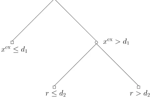
Figure 1. Example of a Binary Tree PartitionP={R1,R2,R3} of the State Space G={(r,ε, h, xex); (r,ε, xex)∈R3, h∈R+}.
However, the parameterization adopted here represents a good trade-off between flexibility and computational feasibility.
The partitionP is constructed on a binary tree where every
terminal node represents a rectangular partition cell Rj, the
edges of which are determined by thresholds. Figure 1 illus-trates an example of a binary tree partition of the state space,
G= {(r, ε,h,xex);(r, ε,xex)∈R3,h∈R+},
which involves three partition cellsR1,R2, andR3. For
sim-plicity and illustration purposes, we assume a one-dimensional exogenous variable xex identified with the long-term interest rate. Each rectangular partition cell R1,R2, and R3
corre-sponds to a terminal node in the tree and determines a regime. The first cell,R1= {(r, ε,h,xex);xex≤d1}, represents a first
regime of rt in response to low long-term interest rates. The second cell, R2= {(r, ε,h,xex);xex>d1andr≤d2},
corre-sponds to a second regime in response to high long-term in-terest rates and low short-term inin-terest rates (i.e., high spreads). Finally,R3= {(r, ε,h,xex);xex>d1andr>d2}represents a
third regime in response to high short-term and long-term inter-est rates.
It is important to bear in mind that the threshold values d1andd2are not restricted and are jointly estimated. Thus, low
(high) interest rates with respect to the partition{R1,R2,R3} is stated not in absolute terms, but rather in terms of interest rates that are sufficiently below (above) the threshold values d1andd2.
The negative log-likelihood for model (10) conditionally on1and on some reasonable starting valueh1(θ )is
wherepZ(·) is the density function of the distribution of the standardized innovationzt andn2= {2, . . . , n}. Therefore, for any given partitionP, model (10) can be estimated by means
of (pseudo) maximum likelihood. The choice between different partition structures (i.e., the selection of the optimal threshold functions) involves a model choice procedure for nonnested hy-potheses. We present some more details on the estimation pro-cedure in the next section.
2.3 The Estimation Procedure
Estimation of the GTS model (11)–(12) works as follows. First, we estimate a largest GTS model, given a maximal num-ber of candidate thresholds. Then we apply a model selection procedure for nonnested models that selects an optimal sub-tree of the largest sub-tree estimated in the first step. This estima-tion procedure closely follows that introduced by Audrino and Bühlmann (2001). Small-sample performance results and relia-bility results of the GTS estimation procedure based on Monte Carlo simulations are summarized in the Appendix.
2.3.1 Growing the “Maximal” Binary Tree. We first fix a
maximal allowed numberM+1 of partition cells in the tree. This corresponds to the maximal number of possible multivari-ate regimes in conditional means and variances. For any co-ordinate axis of the multivariate prediction spaceGthat must be split, we search for multivariate thresholds over grid points that are empirical α-quantiles of the data along the relevant coordinate axis. Typically, we fix the empirical quantiles as
α=i/mesh,i=1, . . . ,mesh−1, where mesh determines the fineness of the grid on which we search for multivariate thresh-olds. Typically, we choose mesh=8.
The partition of the prediction spaceGoft−1= {rt−1, εt−1,
ht−1,xext−1}into a maximal number ofM+1 cells is then
per-formed as follows. A first threshold,d1∈RorR+, in one
com-ponent, indexed by a component indexι1∈ {1, . . . ,p}, withp
the dimension ofG, partitionsGas
G=Rleft∪Rright,
tion>instead of≤. In a second step, one of the partition cells
Rleft orRright is again partitioned with a second thresholdd2
and a second component indexι2in the same way as before.
To iterate this procedure, specifically, for the mth iteration step, we specify a new pair (dm, ιm) that determines a new threshold for the component indexed byιmand an existing par-tition cell that is further split into two subcells. For a new pair
(d, ι)∈R× {1, . . . ,p}, refinement of an existing partitionP(old)
is obtained by pickingRj∗∈P(old)and splitting it as
Rj∗=Rj∗,left∪Rj∗,right. (14)
This gives a new (finer) partition ofGas
P(new)= {Rj,Rj∗,left,Rj∗,right,j=j∗}, (15)
where(d, ι)describes a threshold and a component index such that
Rj∗,left=(r, ε,h,xex)∈Rj∗⊂G;(r, ε,h,xex)ι≤d . (16)
Rj∗,right is defined analogously by the>instead of the ≤
re-lation. The whole procedure finally determines a partitionP= {R1, . . . ,Rk}that can be summarized by a binary tree, where the terminal nodes represent the rectangular partition cells inP
(see Fig. 1).
To select the specific threshold and component index(d, ι)
in each iteration step of the foregoing procedure, we pro-ceed by optimizing the conditional negative (pseudo) log-likelihood (13). Then we obtain a partitionPopt(M)corresponding
to a large binary tree equipped with parameter estimatesθˆ(M).
To end this section, it is important to draw attention to the fact that only the number of estimated thresholds (or, equiv-alently, the number of estimated regimes) in the maximal tree can be arbitrary (high), but the maximal partition cannot be. Be-cause, similar to the classification and regression trees (CART) procedure (Breiman, Friedman, Olshen, and Stone 1984), for computational feasibility, it is not possible to estimate the best partition among all of the possible ones, the proposed procedure is based on a hierarchical strategy. The first split in the binary tree is the one that generates the greatest improvement in min-imizing the conditional negative (pseudo) log-likelihood (13) (i.e., the statistical criterium chosen for predictive accuracy). Then the second split in the tree is the one that added to the (already fixed) first one yields the maximal improvement in minimizing the conditional negative log-likelihood, and so on. At the end, we get a “unique” data-driven maximal par-tition that is optimal with respect to the conditional negative log-likelihood criterion. In other words, the procedure yields a natural ordering of the partition cells (regimes) based on the optimal binary tree structure.
2.3.2 Selection of the Optimal Number of Regimes
(Sub-trees) by Pruning. The maximal binary tree constructed with
the foregoing estimation procedure can be too large, which can lead to overfitting. As with CART, we correct by pruning. Specifically, we search for a best subtree ofPopt(M), and conse-quently we estimate the optimal number of regimes using the Bayes information criterion
BIC(Pi)= −2·ℓ(θˆPi;n
2)+dim(θˆ
Pi)·log(n−1), (17)
whereθˆPi is the implied pseudo–maximum likelihood estimate
for the subtreePi. We finally select the binary tree (or,
equiva-lently, the partition)Pˆthat minimizes (17) across all subtreesPi
of the maximal treePopt(M). Note that the selection of the optimal
subtree is also entirely data-driven.
3. DATA AND ESTIMATION RESULTS
3.1 Data
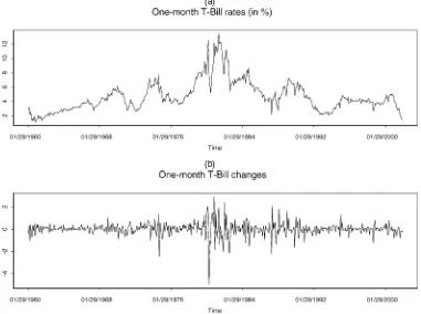
The data used in this study are 1-month U.S. Treasury Bill rates downloaded from the Fama CRSP Treasury bill files. The data span the time period January 1960–December 2001, for a total of 504 monthly observations. Figure 2 plots the data as well as the monthly changes in short-term interest rates. Table 1 presents some sample statistics.
Figure 2 illustrates quite aptly the dramatic changes in the short-term interest rates that occurred during the 1973–1975 OPEC oil crisis and the 1979–1982 Federal Reserve experi-ment. The volatility of the monthly changes associated with the Fed experiment is striking. Volatility was also noticeably higher than average during the 1973–1975 period and immediately af-ter the October 1987 stock market crash. As expected, Table 1 shows that the mean change in the short-term interest rates is close to 0, that there is significant excess kurtosis, and that the correlation betweenrt andrt−1is negative. All of these
styl-ized facts have been documented elsewhere.
To exploit the possible additional information included in the yield curve, we also downloaded the 60-month zero-coupon bond rates from the Fama CRSP discount bond files. Some sam-ple statistics for the 60-month yields, as well as for the spread between long- and short-term rates, are summarized in Table 1.
(a)
(b)
Figure 2. A Time Series of Monthly 1-Month Treasury Bill Rates (in percentages) (a) and the First Differences of This Series (b). The sample period is January 1960–December 2001, for a total of 504 observations.
Table 1. Summary Statistics of Data
Central moments Autocorrelations
Mean SD Skew Kurt Lag 1 Lag 2 Lag 3
1-month rates 4.6573 2.1204 1.2966 5.2241 .9556 .9203 .8875
1-month changes −.0038 .6095 1.0215 15.199 −.1045 −.0332 −.0653
60-month rates 6.9773 2.4603 .9309 3.5981 .9860 .9696 .9541
Spread 2.3200 1.1502 .6745 3.6596 .8723 .8064 .7391
CPI 4.2779 2.8568 1.2667 4.1458 .9909 .9782 .9629
PPI 3.4385 3.7274 1.3461 4.4884 .9843 .9630 .9407
HELP 85.318 22.647 .3225 2.2329 .9880 .9759 .9601
IP 3.1998 4.6552 .8555 3.8134 .9622 .9015 .8288
UE 1.3244 10.117 .5628 4.5274 .9764 .9509 .8581
S&P500 .6939 4.2662 .3433 4.9306 .0093 −.0473 .0120
NOTE: The 1 month yield is from the Fama CRSP Treasury bill files. The 60-month yield is the annual zero coupon bond yield from the Fama CRSP bond files. Spread refers to the difference between long-term and short-term interest rates. The inflation measures CPI and PPI refer to CPI inflation and PPI (Finished Goods) inflation. We calculate the inflation measure at timetusing log(Pt/Pt−12) wherePtis the (seasonal-adjusted) inflation index. The real activity measures HELP, IP, and UE refer to the Index of Help Wanted Advertising in Newspapers, the (seasonal adjusted) growth rate in industrial production and the unemployment rate. The growth rate in industrial production is calculated using log(It/It−12) whereItis the (seasonal-adjusted) industrial production index. S&P500 refers to S&P500 monthly log returns. The sample period is January 1960–December 2001, for a total of 504 observations.
We also use additional macroeconomic variables as con-ditioning predictors in our GTS model, because we believe that they can substantially improve estimation and forecasts. We consider the same macroeconomic variables used by Ang and Piazzesi (2003) in their study. We divide the macroeco-nomic variables into two main groups. The first group consists of two inflation measures based on the CPI and the PPI of fin-ished goods. The second group contains variables that capture real activity: HELP, unemployment (UE), and the growth rate of industrial production (IP). We also consider monthly log re-turns of the S&P500 index. All of the macroeconomic data were downloaded fromDatastream Internationalfor the time period under investigation. This list of variables includes most vari-ables that have been used in the macro literature. Among these variables, HELP is traditionally considered a leading indicator of real activity. Summary statistics of these variables are re-ported in Table 1.
3.2 Regime-Switching Model Estimation Results
We begin our analysis by considering a two-regime RS model (as in Gray 1996), given by (6)–(9), because it can be used as a benchmark model to test the accuracy of the GTS GARCH models. The parameter estimates for this model are given in Table 2. Results are computed for the entire period of January 1960–December 2001, for a total of 504 monthly observations. The detailed specification of the model appears after the table. Standard errors for the parameter estimates are computed using a model-based bootstrap from the standardized residuals (see Efron and Tibshirani 1993 for more details).
Table 2 reports estimates of the two-regime RS model. The estimates of the conditional mean and variance parameters are similar to those found by Gray (1996) and confirm a certain asymmetry across regimes. In the high-volatility and high– interest rates regime (regime 1) there is weak evidence of mean reversion. In contrast, there is no evidence of mean reversion at low and moderate interest rates (coinciding with episodes of regime 2 and lower volatility). As in the results of Gray (1996), the conditional variance appears to separate into GARCH and CIR regimes. In regime 1 the CIR parameter yields the most sig-nificant (although short of 1% confidence level) effect driving
the conditional variance. In regime 2 the most important factor in determining volatility is recent volatility, whereas the para-meter estimate for the level effect is approximately zero.
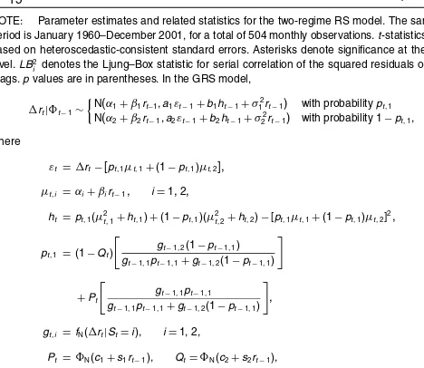
Table 2. RS Parameter Estimates
NOTE: Parameter estimates and related statistics for the two-regime RS model. The sample period is January 1960–December 2001, for a total of 504 monthly observations.t-statistics are based on heteroscedastic-consistent standard errors. Asterisks denote significance at the 1% level.LB2
i denotes the Ljung–Box statistic for serial correlation of the squared residuals out to ilags.pvalues are in parentheses. In the GRS model,
rt|t−1∼
andfNandNare the density and the probability functions of the standard normal distribution.
Within each regime, the GARCH processes are stationary and less persistent than in the single-regime model (ai+bi< .71, i=1,2). Conversely, allowing for regime switches sub-stantially increases the value of the CIR parameter in the high-volatility regime. This illustrates a potential advantage of the RS model over the single-regime model. In the RS model, volatility clustering can be caused by three factors, whereas in the single-regime model the only source of clustering lies in the GARCH process. Because the single-regime model can-not capture the persistence of regimes, all of the persistence in volatility is thrown into the persistence of an individual shock. Consistent with the results of Lamoureux and Lastrapes (1990), individual shocks then appear to take too long to die down to the average variance.
As expected, the RS model does a relatively good job mod-eling the stochastic volatility of short-term interest rates. The Ljung–Box statistics relating to the squared standardized resid-uals indicate no remaining serial correlation.
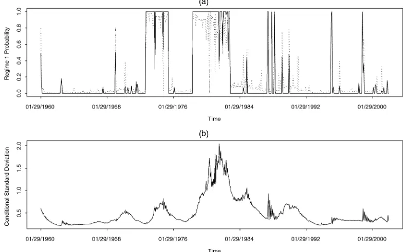
Figure 3(a) plots the ex ante and smoothed probabilities from the two-regime RS model. This figure points to at least three periods during which the process was most likely in the high-variance regime: 1973–1975, 1979–1982, and late 1987 to the first months of 1988. These periods may be explained intuitively. The first and second periods are clearly driven by the OPEC oil crises and by the Federal Reserve experiment; the third period corresponds to the months immediately after the stock market crash of October 1987. Figure 3(b) contains a plot of the conditional standard deviation implied by the two-regime RS model. Once again, the periods of high volatility are particularly apparent.
3.3 Generalized Tree-Structured Model
Estimation Results
In this section we analyze the parameter estimates of the con-ditional mean and variance of the short-term interest rate for two different forms of the GTS model (10) with conditional mean and variance equations specified by (11) and (12).
3.3.1 Simple Generalized Tree-Structured Model. We
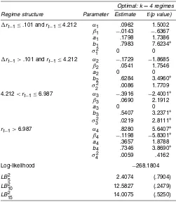
be-gin the analysis of GTS models by considering a model that uses only endogenous information for prediction (i.e., not ex-ploiting the possible additional information included in the term structure or in other macroeconomic variables). We call such a model a simple GTS model. The parameter estimates for this model appear in Table 3. Results are computed for the whole time period of January 1960–December 2001, for a total of 504 monthly observations. The detailed specification of the model is given after the table.
We find that the simple GTS model has four different regimes, endogenously estimated in our procedure. The first two regimes are characterized by low and stable interest rates; however, the short-term interest rate process behaves differ-ently in these two regimes in response to past negative and positive (meaning below or above a given threshold) interest rate changes. In the first regime the tendency of the interest rate process is positive. Negative past interest rate changes act as warning signals that the behavior of the short-term interest rate process may change in reaction to a different monetary policy or to new real activity conditions. The implied long-run mean (−α1/β1) is 6.73% and, because it lies outside the regime
specification, acts as a kind of high external attractor. In this
(a)
(b)
Figure 3. Regime-Switching Model Results. (a) A time series plot of the ex ante (· · · ·) and smoothed ( ——) probabilities that the short rate process is in regime 1 (the high-volatility regime) at time t according to the RS model. The ex ante probability is based on the information available at time t , and the smoothed probability is based on the entire sample. (b) A time series plot of the conditional standard deviation of changes in the short rate based on the RS model. Parameter estimates are based on a dataset of 1-month Treasury Bill rates. The sample period is January 1960–December 2001, for a total of 504 monthly observations.
Table 3. Simple GTS Parameter Estimates
Optimal: k=4 regimes Regime structure Parameter Estimate t|(p value)
rt−1≤.101 andrt−1≤4.212 α1 .0962 1.5002
NOTE: Parameter estimates, regimes structures, and related statistics for the simple GTS model that does not use any additional information included in other term structure and macro-economic variables for prediction. The sample period is January 1960–December 2001, for a total of 504 monthly observations.t-statistics are based on heteroscedastic-consistent standard errors. Asterisks denote significance at the 1% level.LB2
i denotes the Ljung–Box statistic for se-rial correlation of the squared residuals out toilags.pvalues are in parentheses. In the simple GTS model,rt|t−1∼N(µt,ht),
regime the conditional mean expected change is always posi-tive (≥.0962−.0143×4.212=.0359), although the strength of the attraction of the external high long-run mean is low. In fact, when the short rate is 3%, the conditional mean change is.0962−.0143×3=5.33 basis points. When past interest rate changes are negative, the level of the interest rate tends to increase, and the process tends to switch to another regime as-sociated with higher interest rates. In this regime the effect of individual shocks is not large immediately, but is significantly persistent.
In the second regime there is weak evidence of a slow negative mean reversion with respect to a relatively low implied long-run mean (3.19%), which acts as a kind of reflecting barrier because it is rarely below 3.19% in our sample. However, the strength of this reflection is relatively moderate. When the short rate is 4%, the expected change is −.1729+.0541×4=4.35 basis points. In this regime positive past interest rate changes act as good signals from the market.
Once the interest rate falls below the implied long-run mean level, the process switches to regime 1 because we have a neg-ative past interest rate change. As with regime 1, the GARCH parameter estimate in the conditional variance is highly signif-icant. What is different here is that there is also weak evidence that the conditional variance is related to the level of the short rate. Note that although the value of the CIR parameter is small, it is also economically significant.
The third regime is characterized by moderate to high in-terest rates and volatilities. In this regime there is statisti-cal evidence of negative mean reversion. The implied long-run mean is 5.68% and acts as a reflecting barrier. However, the strength of this reflection is moderate; when the short rates are 5% and 6.5%, the conditional mean changes are −4.66 and 5.69 basis points. In this regime, when the short rate is above (below) the implied long-run mean, it tends to increase (decrease) further and to move slowly to the high (low) interest rate regime 4 (regimes 1 and 2). Both CIR and GARCH para-meters are found to be statistically significant.
The fourth and last regime is characterized by high inter-est rates and volatilities. Analogously to regime 1, the implied long-run mean is 6.91%, and, because it lies outside the regime specification, it acts as a kind of low external attractor. In this regime the conditional mean expected change is always neg-ative, with a tendency to reduce the level of the short rates. Unlike in regime 1, here the speed of the conversion to the ex-ternal low implied long-run mean is high. Moreover, the para-meter estimates of the conditional mean are found to be highly statistically significant. Individual shocks have a large immedi-ate and persistent effect on the conditional variance. Within this regime, the GARCH process is not stationary (a4+b4>1).
However, as shown more clearly in Figure 4, this regime char-acterizes only particular events like the 1979–1982 Federal Re-serve experiment.
In summary, we find statistical evidence of the existence of more than two asymmetric threshold regimes. The behavior of the short rate process is different in each regime. In contrast to single-regime models, using our approach, we are able to differ-entiate the different sources of volatility persistence. Moreover, similar to the two-regime RS model, our results suggest that the mean reversion, which is assumed by many models to be operating continuously, in fact does not occur in the different regimes. However, the global behavior of the conditional mean estimated using the simple GTS model is similar to that of a mean-reverting process.
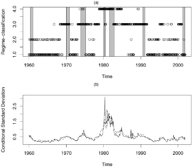
As expected, the simple GTS model is quite suitable for mod-eling the stochastic volatility of short-term interest rates. The Ljung–Box statistics relating to the squared standardized resid-uals indicate no remaining serial correlation. Figure 4(a) plots the regime classification of the observations from the simple GTS model. The detailed specification of each regime appears after the figure. Shaded NBER recessions are overlaid to depict corresponding recessions/expansions.
Although regime 1 and regime 2 have different economic and statistical characteristics, they are both associated with time pe-riods of low and stable interest rates. This is also shown in Fig-ure 4. For example, observations belonging to the 1961–1969 and the 1991–2001 periods are in general classified in regimes 1 and 2 according to the simple GTS model. Regime 3 is charac-terized by moderate to high interest rates and volatilities and is
(a)
(b)
Figure 4. Simple GTS Model Results. (a) A time series plot of the regime classification of the observation at time t (i.e., It={1, 2, 3, 4}) according
to the simple GTS model. Shaded NBER recession periods are overlayed to see regime correspondence with recessions/expansions. The regime classification is based on the endogenous information available at time t−1, without including additional information from the term structure or other macroeconomic variables. (b) A time series plot of the conditional standard deviation of changes in the short rate based on the simple GTS model ( ——) superimposed on those from a two-regime RS fit (dotted line) for comparison. Parameter estimates are based on a dataset of 1-month Treasury Bill rates. The sample period is January 1960–December 2001, for a total of 504 monthly observations. Optimal regimes of the simple GTS model are as follows: Regime 1:R1={∆rt−1≤.101 and rt−1≤4.212}; regime 2:R2={∆rt−1>.101 and rt−1≤4.212}; regime 3: R3={4.212<rt−1≤6.987}; regime 4:R4={rt−1>6.987}.
mostly associated with particular episodes like the 1973–1975 OPEC oil crises and the years after the market crash of Oc-tober 1987. During these periods, more than 75% of the ob-servations are classified in regime 3. Finally, the 1979–1982 Federal Reserve experiment and the short peak corresponding to the end-year of October 1987 are episodes classified in the high-volatility regime 4.
Figure 4(b) plots the conditional standard deviation implied by the simple GTS model superimposed on those from a two-regime RS fit for comparison purposes. Once again, periods of high, moderate, and low volatility are particularly apparent. Volatility dynamics from both models are similar. Summariz-ing, Figure 4 highlights that particular episodes and different business cycles coincide with the different regimes estimated using the simple GTS model. In contrast to the two-regime RS model, we find that observations occurring at the time of the Federal Reserve experiment and the OPEC oil crisis are not classified in the same regime.
To end this section, we analyze the correspondence be-tween model-implied regimes and business cycles. To more formally characterize the correspondence of NBER
reces-sions/expansions with the model-implied regimes, we report frequency of the regimes in recessions versus expansions. The results are summarized in Table 4.
Table 4. Frequency of the Different Regimes in NBER Recessions and Contractions
Frequency
Regime Total Contraction Expansion
Frequency of simple GTS regimes in recession and expansions 1 195/504=.387 10/75=.133 185/429=.431
2 73/504=.145 5/75=.067 68/429=.159
3 173/504=.343 40/75=.533 133/429=.310
4 63/504=.125 20/75=.267 43/429=.100
Frequency of full GTS regimes in recession and expansions
1 255/504=.506 56/75=.746 199/429=.463
2 31/504=.062 0/75=0 31/429=.072
3 70/504=.138 0/75=0 70/429=.163
4 148/504=.294 19/75=.254 129/429=.302
NOTE: The sample period is January 1960–December 2001, for a total of 504 monthly obser-vations. Total (number of observations in the regime/total number of observations), contraction (number of contraction observations in the regime/total number of contraction observations), and expansion (number of expansion observations in the regime/total number of expansion observations) frequencies for the simple and full GTS models are reported.
Both Figure 4 and Table 4 provide empirical evidence that some of the regimes can be closely related to business cy-cles. In particular, 80% of the recession observations belongs to regimes 3 and 4. This result is consistent with previous em-pirical evidence (see, e.g., Ang and Bekaert 2002); recessions are characterized by significantly higher short-term and some-what more variable interest rates. Only the recession in the early 1960s and the last recession in 2001 are characterized by low interest rates. In contrast, most time periods coinciding with regimes 1 and 2 can be closely associated with long expansions. Similar to Bansal and Zhou (2002) and Bansal et al. (2004), we compute correlations between yield spreads and indicators for model-implied regimes and NBER cycles. Note, however, that the simple GTS model does not use additional informa-tion included in the term structure. The correlainforma-tions between yield spreads and NBER and simple GTS regime indicators are
.135 and.153, in line with the results reported in the aforemen-tioned studies. The correlation between NBER indicator and the simple GTS regime indicator is.216, confirming some signifi-cant relationship between regimes and business cycles.
3.3.2 Full Generalized Tree-Structured Model. To end
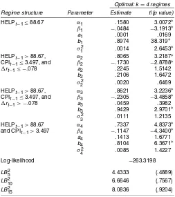
our analysis, we consider a full GTS model that also uses the possible additional information included in the term struc-ture and in other relevant macroeconomic variables for pre-diction. All variables considered in the estimation of the full GTS model are listed in Table 1. The parameter estimates for this model are given in Table 5. Results are computed for the whole time period of January 1960–December 2001, for a total of 504 monthly observations. The detailed model specifications are given after Table 5.
Once again, we find that the estimated full GTS model has four regimes. However, these regimes are characterized differ-ently from those estimated in the simple GTS model and lead to different economic and statistical interpretations.
The first regime is characterized by low real activity. Typical episodes in regime 1 are periods of low and stable inter-est rates. In this regime the implied long-run mean is rela-tively low (3.26%), and there is statistical evidence of mean reversion. The speed of the reversion is moderate; when the short rates are 2% and 6%, the conditional mean changes are 6.12 and −13.24 basis points. As in the case with the low-volatility regime in the two-regime RS model, individual shocks have a small immediate effect on the conditional variance but are strongly persistent. Analogously to regime 2 in the simple GTS model, the conditional variance is also significantly related to the level of the short rate. But in this case, the small value of the CIR parameter makes it economically insignificant.
The second and third regimes are characterized by high real activity and low inflation. Yet the short-term interest rate process behaves differently in these two regimes in response to past negative and positive interest rate changes. The con-ditional mean behavior in regimes 2 and 3 is essentially the same. In both regimes, there is statistical evidence of a fast mean reversion around a moderate implied long-run mean (4.66% and 3.74% per annum in regimes 2 and 3). Nev-ertheless, the conditional variance dynamics are completely different. In regime 2 individual shocks have an immediate im-pact on the conditional variance but die out quickly, whereas in regime 3 individual shocks have a small immediate effect on the
Table 5. Full GTS Parameter Estimates
Optimal: k=4 regimes Regime structure Parameter Estimate t|(p value)
HELPt−1≤88.67 α1 .1580 3.0072∗
NOTE: Parameter estimates, regimes structures, and related statistics for the full GTS model that uses the additional information included in the term structure and in other macroeconomic variables for prediction (xex
t−1). The sample period is January 1960–December 2001, for a total of
504 monthly observations.t-statistics are based on heteroscedastic-consistent standard errors. Asterisks denote significance at the 5% level.LB2
i denotes the Ljung–Box statistic for serial correlation of the squared residuals out toilags.pvalues are in parentheses. In the full GTS model,rt|t−1∼N(µt,ht),
conditional variance but are significantly persistent. This differ-ence can be economically interpreted as follows. In regime 2 past negative interest rate changes may act as warning signals that the behavior of the short-term interest rate process can change. This may be due to a different monetary policy affect-ing the level of the short rate and on inflation and/or to a wors-ening of the production conditions with a consequent reduction of real activity. In other words, the uncertainty about the future behavior of the interest rate process increases, as does the im-mediate impact of individual shocks. In contrast, in regime 3 past positive interest rate changes are seen as good signals. For this reason, the impact of individual shocks is not large imme-diately but is strongly persistent. In both regimes the CIR para-meter is not statistically or economically significant.
The fourth regime is characterized by high real activity and high inflation. In this regime interest rates and volatility are gen-erally high. There is strong evidence of mean reversion around a relatively high implied long-run mean (6.39%). The speed of the reversion is high, although not as high as in regimes 2 and 3.
Similar to the high-volatility regime 4 in the simple GTS model, the conditional variance is not significantly related to the level of the short rate. Individual shocks have a moderate immediate impact and are strongly persistent, although less so than in the low-volatility regime 1.
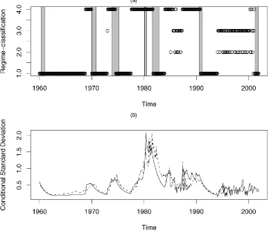
As expected, the full GTS model is very appropriate for modeling the stochastic volatility of the short-term interest rate process. The Ljung–Box statistics relating to the squared stan-dardized residuals indicate no remaining serial correlation. Fig-ure 5(a) plots the regime classification of the observations from the full GTS model. The specification of each regime is de-tailed after the figure. Once again, we overlay shaded NBER recessions to depict recession/expansion correspondence.
Figure 5 clearly shows that regime 1 is associated with time periods of low and stable interest rates. Although regime 2 and regime 3 have different economic and statistical characteristics, they both appear in the same two time periods characterized by low inflation and high real activity. Observations belong-ing to the 1985–1987 and 1994–2000 periods are classified in regimes 2 and 3 according to the full GTS model. Finally, the first half of the 1973–1975 period, the 1979–1982 Federal Re-serve experiment, and the years after the stock market crash
of October 1987 are episodes classified in the high-volatility, high-inflation, and high–real activity regime 4.
Figure 5(b) plots the conditional standard deviation implied by the full GTS model superimposed on those from an extended two-regime RS fit (see Sec. 4) for comparison. Once again, pe-riods of high and low volatility are particularly apparent. Com-paring the volatility estimates from the full GTS model with those from the two-regime RS model, we see some important differences in the volatility dynamics, particularly during the 1979–1982 Federal Reserve experiment period and the months after the stock market crash of October 1987. This is a conse-quence of the different approaches used to estimate the regimes in the models. As we show in the following out-of-sample ex-periments, these differences will prove crucial in issuing accu-rate volatility forecasts.
Similar to what we did in the last section, we analyze the correspondence between model-implied regimes and business cycles. Frequency of the full GTS regimes in recessions versus expansions are summarized in Table 4.
Table 4 and Figure 5 clearly show that estimated regimes from the full GTS model and NBER contractions/expansions
(a)
(b)
Figure 5. Full GTS Model Results. (a) A time series plot of the regime classification of the observation at time t (i.e., It={1, 2, 3, 4}) according to
the full GTS model. Shaded NBER recession periods are overlayed to see regime correspondence with recessions/expansions. The regime classifi-cation is based on all available information at time t−1, also including additional information from the term structure and other macroeconomic vari-ables introduced in Table 1. (b) A time series plot of the conditional standard deviation of changes in the short rate based on the full GTS model ( —–) superimposed on those from an extended two-regime RS fit (see Sec. 4;· · · ·) for comparison. Parameter estimates are based on a dataset of 1-month Treasury Bill rates. The sample period is January 1960–December 2001, for a total of 504 monthly observations. Optimal regimes of the full GTS model are as follows: Regime 1:R1={HELPt−1≤88.67}; regime 2:R2={HELPt−1>88.67, CPIt−1≤3.497, and∆rt−1≤ −.078};
regime 3:R3={HELPt−1>88.67, CPIt−1≤3.497, and∆rt−1>−.078}; regime 4:R4={HELPt−1>88.67 and CPIt−1>3.497}.
are related. Most of the contraction observations are character-ized by low or significant drops in real activity. In fact, con-tractions occur mostly during or before time periods associated with regime 1. Moreover, as expected, we find that regimes 2 and 3 (characterized by low inflation and high real activity) closely coincide with long expansions.
Following Bansal and Zhou (2002) and Bansal et al. (2004), we compute correlations between yield spreads, HELP and CPI, and indicators for model-implied regimes and NBER cycles. Note that in our case yield spreads were not chosen as tors in the estimation procedure. The most important predic-tors are HELP and CPI; however, we compute correlations with respect to yield spreads to be consistent with previous litera-ture. Absolute correlations between yield spreads, HELP and CPI, and the NBER indicator are.135,.239, and.355. Conse-quently, the macroeconomic variables seem to be more closely related to business cycles than yield spreads. Correlation be-tween the NBER indicator and the full GTS regime indicator is.245, confirming a significant relationship between regimes and business cycles. Moreover, because the full GTS regimes are constructed using HELP and CPI, the model-implied regime indicator is strongly correlated with such indices (with correla-tions of about.7–.8).
4. THREE OUT–OF–SAMPLE EXPERIMENTS
In this section we investigate whether the introduction of multiple regimes in the GTS models leads to overfitting. This can be easily determined by performing a series of out-of-sample tests. Moreover, using such tests, we are also able to establish the economic significance of allowing for more than one regime. In performing the out-of-sample tests, we estimate the parameters of each particular model over an in-sample pe-riod and compute time series of conditional mean and variances over a subsequent out-of-sample period, holding the estimated parameters and regime structure fixed.
We always compare goodness-of-fit results of the simple and full GTS models with those of (a) the classical random walk, (b) an AR–GARCH model, (c) a two-regime RS model, and (d) an extended two-regime RS model, where the time-varying transition probabilities are also allowed to depend on further ex-ogenous (macroeconomic) variables. In particular, the extended two-regime RS model appears as follows. We consider the same Gray two-regime RS model in (6)–(9), but we extend the time-varying transition probabilitiesPtandQtin
pt,1=(1−Qt) is the density of a Gaussian variable with conditional meanµt,j and conditional varianceht,j. The chosen extended two-regime
RS specification uses the exogenous variablexex(among all of the possible candidates), which minimizes the negative condi-tional maximum likelihood.
Finally, we compare goodness-of-fit results of the simple and full GTS models with those of the realized volatility AR–GARCH model proposed by, among others, Andersen et al. (1999, 2001). To estimate the realized volatility AR–GARCH model, we download daily 1-month interest rate data from the CRSP database. Unfortunately, daily data have been collected only since January 1970. For this reason, our out-of-sample performance tests cover the time period Janu-ary 1970–December 2001, for a total of 7,979 daily observa-tions and 384 monthly observaobserva-tions.
Analogously to the work of Gray (1996), we quantify the goodness of fit of the different models for estimating and pre-dicting monthly conditional first and second moments by means of various measures. Because the conditional variance is an ex-pectation of squared innovations to the interest rate process, we compare volatility estimates from the different approaches to the actual squared innovations. The difference between volatil-ity estimates and actual squared innovations is computed for the in-sample estimation period and for the out-of-sample back-testing period. This difference is then summarized in the form of root mean squared errors (RMSEs), mean absolute errors (MAEs), and the R2 between actual volatility and estimated volatility. Mathematically speaking, we consider
TheR2measure, in providing a direct measure of the goodness of fit of the estimate, differs from theR2measure that would be obtained by projecting actual volatility on forecast volatility. It imposes an intercept at 0 and a slope of 1 on such projection, permitting direct conclusions about a particular estimate rather than about some linear transformation of that estimate.
Because we are also interested in the accuracy of the different models in predicting conditional first moments, we also com-pute classical in-sample and out-of-sample MAE and RMSE statistics for the estimated innovationsǫˆt=rt− ˆµt. In addi-tion to these performance measures, we also consider the nega-tive log-likelihood computed for the out-of-sample period.
Tables 6 and 7 give performance results of three different out-of-sample tests for conditional mean and volatility predictions constructed using an AR–GARCH model, the two-regime and extended two-regime RS models, the simple and full GTS mod-els, and the realized volatility AR–GARCH model. Results for conditional volatility measures are not reported for the simple random walk, because they are always significantly worse (in-sample and out-of-(in-sample) than the AR–GARCH model. In-stead we report the performance results from the random walk
Table 6. Out-of-Sample Specification Tests (conditional mean)
In-sample Out-of-sample
(January 1970–December 1978) (January 1979–December 2001)
Model RMSE MAE RMSE MAE
108 observations 276 observations
AR–GARCH .6326 .4353 .7706 .4381
Two-regime RS .6246 .4266 .7942 .4655
Simple GTS .6246 .4370 .7886 .4342
Extended RS .6231 .4273 .7896 .4621
Full GTS .5452 .3875 .7647 .4304
RW .6283 .4280 .7664 .4379
144 observations 240 observations
AR–GARCH 1.0096 .6328 .5022 .3238
Two-regime RS 1.0023 .6327 .5173 .3375
Simple GTS .9958 .6301 .5027 .3383
Extended RS .9690 .6104 .5086 .3367
Full GTS .9671 .5973 .4853 .3038
RW 1.0069 .6369 .5034 .3351
288 observations 96 observations
AR–GARCH .8262 .5141 .2867 .1790
Two-regime RS .8216 .5087 .2851 .1773
Simple GTS .8148 .5094 .2859 .1789
Extended RS .8207 .5086 .2873 .1792
Full GTS .8239 .5115 .2485 .1735
RW .8254 .5184 .2940 .1893
NOTE: Predictive performance measures for the standard random walk (RW), an AR–GARCH model, regime and extended two-regime RS models, simple and full GTS models. The table reports RMSEs and mean absolute errors MAEs of the innovationsεt=rt−µt. Parameters are estimated over the in-sample period, and held fixed over the out-of-sample period. The data are monthly observations of 1-month Treasury Bill yields. The sample period is January 1970–December 2001, for a total of 384 observations.
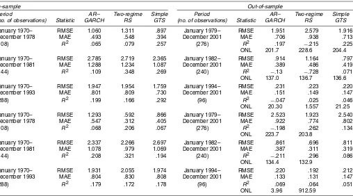
Table 7. Out-of-Sample Specification Tests (volatility)
In-sample Out-of-sample
Period AR– Two-regime Simple Period AR– Two-regime Simple
(no. of observations) Statistic GARCH RS GTS (no. of observations) Statistic GARCH RS GTS
January 1970– RMSE 1.060 1.311 .897 January 1979– RMSE 1.951 2.579 1.916
December 1978 MAE .493 .548 .394 December 2001 MAE .706 .938 .713
(108) R2 .065 .079 .257 (276) R2 .197 −.215 .225
ONL 201.7 228.6 204.4
January 1970– RMSE 2.785 2.719 2.365 January 1982– RMSE .914 1.164 .797
December 1981 MAE 1.288 1.234 1.087 December 2001 MAE .389 .486 .419
(144) R2 .109 .348 .269 (240) R2 −.13 −.728 .071
ONL 137.0 136.7 136.6
January 1970– RMSE 1.947 1.954 1.759 January 1994– RMSE .231 .223 .220
December 1993 MAE .801 .809 .730 December 2001 MAE .151 .149 .147
(288) R2 .199 .166 .292 (96) R2 −.047 .025 .046
ONL 20.30 1.557 21.25
January 1970– RMSE 1.293 .592 .866 January 1979– RMSE 2.523 1.923 2.540
December 1978 MAE .547 .312 .405 December 2001 MAE .922 .774 .802
(108) R2 .068 .206 .067 (276) R2 −.198 .262 .134
ONL 223.7 203.8
January 1970– RMSE 2.337 2.266 2.697 January 1982– RMSE .861 .696 .811
December 1981 MAE 1.078 .979 1.069 December 2001 MAE .387 .311 .319
(144) R2 .208 .321 .194 (240) R2 −.211 .296 .086
ONL 134.4 132.9
January 1970– RMSE 1.931 2.055 1.974 January 1994– RMSE .220 .192 .212
December 1993 MAE .804 .830 .808 December 2001 MAE .133 .131 .147
(288) R2 .179 .172 .178 (96) R2 .069 .064 .051
ONL 3.96 912.59
NOTE: Predictive performance measures for an AR–GARCH model, two-regime and extended two-regime RS models, simple and full GTS models, and the realized volatility AR–GARCH model estimated on daily data. The table reports RMSEs, mean absolute errors MAEs, andR2between actual volatilityε2
t, whereεt=rt−µt, and the conditional varianceht. In addition, we also consider as a measure of predictive performance the out-of-sample negative likelihood (ONL). Parameters are estimated over the in-sample period, and held fixed over the out-of-sample period. Low is better for all statistics except theR2. NegativeR2values result when incorporating the forecast results in an unexplained sum of squares (the square of the difference between actual and
forecast volatility) that is higher than the original total sum of squares (the square of the actual volatility). This occurs, for example, when the estimation period has much higher volatility than actually occurs over the out-of-sample period. In this case, the squared difference between forecast and actual volatility can be very large relative to the squared actual volatility over the out-of-sample period. The data are monthly observations of 1-month Treasury Bill yields. The sample period is January 1970–December 2001, for a total of 384 observations.
for estimating and predicting conditional first moments. Sim-ilarly, we do not report results for conditional mean measures for the realized volatility AR–GARCH model, because these are not significantly different from those obtained using a stan-dard AR–GARCH model.
Analogously to the work of Gray (1996), in the first test the models are estimated from the start of the sample up to the Federal Reserve experiment, a period that includes the OPEC oil crisis. The out-of-sample period includes the whole Federal Reserve experiment, the 1987 market crash, and the subsequent period characterized by an average low volatility through to the end of the sample period. In this test the simple random walk is slightly better than the AR–GARCH model for estimation and prediction of the conditional drift. The optimal GTS mod-els have two regimes: the simple GTS model in response to past short-term interest rates above and below a 8.0125 thresh-old and the full GTS model in response to past HELP values above and below a 86.16 threshold value. Both GTS models perform well in this experiment, with a slight advantage of the full GTS model over the simple GTS model, particularly in pre-dicting conditional first moments. The parameters of the high-volatility regime in both models are well identified by the oil shock. In contrast, two-regime RS models perform very poorly in this experiment. They predict overly high levels of volatility in the low-volatility regime, whereas interest rates turn out to be very stable. This results in high forecast errors and a neg-ative R2. Moreover, both models are clearly outperformed by the AR–GARCH model over the out-of-sample period. This problem does not seem to depend on overfitting, because the in-sample statistics are also better for the AR–GARCH model. In contrast, this can be due to the very short estimating pe-riod, consisting only of 108 monthly observations. Something similar happens with the realized volatility model; it yields no better out-of-sample results than the AR–GARCH model. Differences between the models are smaller when considering performance measures for conditional first moments. Only the full GTS model shows some advantage over the AR–GARCH model.
For the second test, the models are estimated over the first half of the sample and predictions are attempted over the second half of the sample. The in-sample estimation period includes the 1973–1975 period (OPEC oil crises) and part of the Fed-eral Reserve experiment. The out-of-sample period includes the remainder of the Federal Response experiment and the stock market crash of October 1987. In this experiment the in-sample period is significantly more volatile than the out-of-sample pe-riod (with sample variances of the short rate changes in the two periods of 1.037 and.242). Single-regime models perform quite similar in estimating and forecasting conditional drift. The simple GTS model has two optimal regimes in response to past short-term interest rate levels. The full GTS model has three optimal regimes in response to past HELP and CPI val-ues and clearly outperforms all of the alternative competitors. Similar to the first test, all of the RS models have overfitting problems and yield bad volatility predictions. Extending the RS model to incorporate additional (macroeconomic) information achieves some significant out-of-sample improvements over the two-regime RS model. Nevertheless, the extended two-regime RS specification also exhibits a negativeR2. It seems here that
two regimes are not sufficient to accurately forecast the condi-tional variances of the interest rate process. The realized volatil-ity model works quite well but is clearly outperformed by the full GTS model. As before, differences in forecasting condi-tional first moments are smaller; only the full GTS model shows some significant advantage over all competitors.
The final test examines the short-term forecasting ability of the model in estimating the models over the entire sample ex-cept for the last 8 years. The in-sample period is once again significantly more volatile than the out-of-sample period (with sample variances of the short rate changes in the two periods of .693 and .081). Thus the sample variance of the short rate changes is more than eight times larger in the in-sample period than in the out-of-sample period. The simple random walk is clearly beaten by the AR–GARCH model. Once again, the op-timal full GTS model has more than two regimes (three in this case) in response to past short-term and long-term interest rate levels. All of the models perform well in this experiment, ex-cept for the AR–GARCH model, which shows a negativeR2. The extended RS and the full GTS models show the best out-of-sample results.
In summary, the GTS models perform well in all three tests with respect to four different performance measures for con-ditional first and second moments. The full GTS model that also uses additional (macroeconomic) information for predic-tion clearly outperforms all of the alternative competitors (in-cluding the simple GTS model). In contrast, in some cases the RS models yield predictions that are not accurate enough. This shortcoming is not corrected when incorporating addi-tional exogenous information for prediction into the RS model. Our full GTS model also outperforms the realized volatility AR–GARCH model that uses information of daily recorded 1-month short-rate data for predicting monthly conditional first and second moments. The realized volatility model works quite well in the different out-of-sample experiments, but, because it assumes fixed parameters for the whole sample, is not able to completely capture the time-varying behavior of the short-rate process. Single regimes are clearly outperformed; for a suffi-ciently long in-sample period, the AR–GARCH model perform better in forecasting both conditional first and second moments than a standard random walk. We conclude that the description of the short-rate process switches in general between more than two regimes characterized by past values of multivariate en-dogenous and exogenous (macroeconomic) predictor variables lying below (or above) some estimated thresholds. Moreover, volatility forecast from the RS models can be considerably im-proved using the GTS approach and may be profitably used in the valuation of interest rate–sensitive securities and interest rate management.
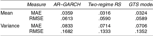
To end this section, we performed a series of equal predictive ability (EPA) tests for forecasting conditional first and second moments to quantify statistically differences between the per-formances of the simple and full GTS models. In particular, we used the EPA tests introduced by Diebold and Mariano (1995) and Audrino and Trojani (2006) for differences of performance terms. With respect to most of the performance measures con-sidered in this study, we found that the null hypothesis of EPA is strongly rejected at the 5% confidence level, preferring the full over the simple GTS model as a forecasting model for the short-rate dynamics.