Manajemen | Fakultas Ekonomi Universitas Maritim Raja Ali Haji jbes%2E2011%2E10278

(1)

Full Terms & Conditions of access and use can be found at

http://www.tandfonline.com/action/journalInformation?journalCode=ubes20

Download by: [Universitas Maritim Raja Ali Haji] Date: 11 January 2016, At: 22:28

Journal of Business & Economic Statistics

ISSN: 0735-0015 (Print) 1537-2707 (Online) Journal homepage: http://www.tandfonline.com/loi/ubes20

Reality Checks and Comparisons of Nested

Predictive Models

Todd E. Clark & Michael W. McCracken

To cite this article: Todd E. Clark & Michael W. McCracken (2012) Reality Checks and

Comparisons of Nested Predictive Models, Journal of Business & Economic Statistics, 30:1, 53-66, DOI: 10.1198/jbes.2011.10278

To link to this article: http://dx.doi.org/10.1198/jbes.2011.10278

View supplementary material

Published online: 06 Apr 2012.

Submit your article to this journal

Article views: 271

View related articles

(2)

Supplementary materials for this article are available online. Please go to www.tandfonline.com/r/JBES

Reality Checks and Comparisons of Nested

Predictive Models

Todd E. CLARK

Economic Research Dept., Federal Reserve Bank of Cleveland, P.O. Box 6387, Cleveland, OH 44101 (todd.clark@clev.frb.org)

Michael W. MCCRACKEN

Research Division, Federal Reserve Bank of St. Louis, P.O. Box 442, St. Louis, MO 63166 (michael.w.mccracken@stls.frb.org)

This article develops a simple bootstrap method for simulating asymptotic critical values for tests of equal forecast accuracy and encompassing among many nested models. Our method combines elements of fixed regressor and wild bootstraps. We first derive the asymptotic distributions of tests of equal forecast accu-racy and encompassing applied to forecasts from multiple models that nest the benchmark model—that is, reality check tests. We then prove the validity of the bootstrap for these tests. Monte Carlo experiments indicate that our proposed bootstrap has better finite-sample size and power than other methods designed for comparison of nonnested models. Supplementary materials are available online.

KEY WORDS: Equal accuracy; Forecast evaluation; Prediction.

1. INTRODUCTION

With improvements in computational power, it has become increasingly straightforward to mine economic and financial datasets for variables that might be useful for forecasting. This point has been made clearly by numerous authors, including Denton (1985), Lo and MacKinlay (1990), and Hoover and Perez (1999). In light of this data mining, it is clear that the search itself must be taken into account when attempting to validate whether any of the findings are statistically significant. Various methods are available to manage this multiple-testing problem, including the traditional use of Bonferroni bounds as well as more recent methods involvingq-values (Storey 2002). The bootstrap is a particularly tractable method of manag-ing this multiple-testmanag-ing problem. Specifically, in the context of out-of-sample tests of predictive ability, White (2000) de-veloped a bootstrap method of constructing an asymptotically valid test of the null hypothesis that forecasts from a potentially large number of predictive models are as accurate as those from a baseline model. Research since has extended the applicability of White’s results. Hansen (2005) showed that normalizing and recentering the test statistic in a specific manner can lead to a more accurately sized and powerful test. Corradi and Swanson (2007) provided important modifications that permit situations in which parameter estimation error enters the asymptotic dis-tribution.

One thing that the existing bootstrap reality checks have in common is the assumption that the baseline model is nonnested with at least one of the competing models. More precisely, they require that the (M×1)vector of out-of-sample averages of the loss differentials (each element of the vector is the average difference in forecast accuracy between the baseline and a dis-tinct competing model) is asymptotically normal with a positive semidefinite long-run covariance matrix. Along with additional moment and mixing conditions, this condition on the long-run covariance matrix is satisfied if at least one of the models is nonnested with the baseline.

However, in many forecast comparisons, the baseline model is a simpler, nested version of all of the competing models. The purpose of such a comparison is to determine whether the ad-ditional predictors associated with the larger models improve forecast accuracy relative to the restricted baseline. In general, in asset return applications, economic theories of efficient mar-kets imply that excess returns form a martingale difference and a null hypothesis under which all predictive models nest the baseline model of zero expected return. In macroeconomic ap-plications, it is standard to examine the predictive content of some variable for output or inflation by comparing a baseline autoregressive model to alternative models that add in lags of other potential predictors. Examples in the literature include Cheung, Chinn, and Pascual’s (2005) examination of various exchange rate models, Goyal and Welch’s (2003, 2008) studies of the predictive content of various business fundamentals for stock returns, and Stock and Watson’s (1999, 2003) analyses of output and inflation forecasting models.

In such evaluations of multiple forecasting models that nest the benchmark model, the results of studies such as that of White (2000) on the asymptotic and finite-sample properties of bootstrap-based joint tests of equal forecast accuracy, based on nonnested models, may not apply. Intuitively, with nested models, the null hypothesis that the restrictions imposed in the benchmark model are true implies that the population errors of all of the competing forecasting models are exactly the same. This in turn implies that the population difference between the competing models’ mean square forecast errors is exactly zero, with zero variance. As a result, the distribution of at-statistic for equal mean squared error (MSE) may be nonstandard. Indeed, Clark and McCracken (2001, 2005) and McCracken (2007)

53

(3)

showed that for pairs of forecasts from nested models, the dis-tributions of tests for equal forecast accuracy typically are not normally distributed.

Motivated by the frequency with which researchers compare predictions from a baseline nested model with many alternative nesting models, this article develops a novel, simple bootstrap that can be used to construct joint tests of equal out-of-sample forecast accuracy or forecast encompassing among such fore-casts.

Before proceeding, we should make clear our contribution to the literature on simulation-based methods for multiple test-ing. Hansen (2005) noted explicitly that his results and the re-sults of White (2000) do not apply when the baseline model is nested by all of its competitors. For the case of a small set of nested models, Hubrich and West (2010) proposed compar-ing an adjustedt-test for equal MSE (equivalently, at-test for forecast encompassing) against the simulated maximum of a set of standard normal random variables. Their approach is based on the observation of Clark and West (2007) that, although the true asymptotic distributions of the t-tests are not normal under general conditions, the distributions often can be rea-sonably approximated by the standard normal. Inoue and Kil-ian (2004) explicitly derived the asymptotic distribution of two tests for equal population-level out-of-sample predictive ability when the baseline model is nested by many competing mod-els, both of which we consider here. Our article extends the work of Inoue and Kilian (2004) in three dimensions. First, we provide analytics for two more tests. Second, we extend the re-sults of Inoue and Kilian (2004) to environments that allow for forecast horizons greater than one period and conditionally het-eroscedastic errors. Finally, and most importantly, we develop a fixed regressor bootstrap method for obtaining asymptotic crit-ical values under the null of equal accuracy at the population level, and we prove the validity of the bootstrap.

Although our results apply only to a setup that some might see as restrictive—direct multistep (DMS) forecasts from nested models—the list of studies analyzing such forecasts sug-gests that our results should be useful to many researchers. Re-cent applications considering a variety of DMS forecasts from nested linear models include, among others, the studies cited at the beginning of this section and studies by Hong and Lee (2003), Mark (1995), Kilian (1999), Sarno, Thornton, and Va-lente (2005), Cooper and Gulen (2006), Rapach and Wohar (2006), Bruneau et al. (2007), Moench (2008), Hendry and Hubrich (2011), and Molodtsova and Papell (2009).

This article is organized as follows. After introducing es-sential notation and the forecast-based tests considered, Sec-tion 2 presents the tests considered and our proposed bootstrap method. Section 3 derives the asymptotic distributions of the tests and proves the validity of the bootstrap. Section 4 presents Monte Carlo results on the finite-sample performance of our proposed bootstrap compared to some other methods. Section 5 applies our tests to forecasts of commodity prices and GDP growth in the United States. Section 6 concludes.

2. A BOOTSTRAP FOR NESTED MODEL

REALITY CHECKS

In this section we describe essential notation and the forecast test statistics considered, then present our proposed bootstrap algorithm.

tor of additional covariates,xM¯,t. The set of predictorsxt may

include lags ofyt. Subvectors ofxM¯,tdifferentiate the

compet-ing unrestricted models. Thus there exist 2kM¯ −_{1 unique} un-restricted linear regression models that nest the baseline model within it. Letj=1, . . . ,M denote an index of the collection ofM≤2kM¯ −_{1 unique models}_x′

j,tβjto be compared with the

baseline nested modelx′₀_,_tβ₀.

At every forecast origin, each of the forecasting models is estimated by ordinary least squares (OLS), yielding coeffi-cients βˆ_j_,_t. The τ-step-ahead forecast errors for model j are

ˆ

uj,t+τ =(yt+τ−x′j,tβˆj,t),j=0,1, . . . ,M. Because the models

are nested, the null hypothesis that the additional predictors do not provide predictive content implies that the population fore-cast errorsuj,t+τ≡(yt+τ−x′_j_,_tβj)satisfyuj,t+τ=u0,t+τ≡ut+τ

for allj=1, . . . ,M.

2.2 Test Statistics

We consider a total of four forecast-based tests: two tests of equal forecast accuracy and two tests for forecast encom-passing. In particular, we consider multiple-model variants of thet-statistic for equal MSE developed by Diebold and Mar-iano (1995) and West (1996) and theF-statistic proposed by McCracken (2007). We also consider multiple-model variants of thet-statistic for encompassing developed by Harvey, Ley-bourne, and Newbold (1998) and West (2001) and the variant proposed by Clark and McCracken (2001). Applying the tests to multiple models involves taking the maximum of test statis-tics formed for each alternative model forecast relative to the benchmark model forecast.

The two tests of equal MSE are based on the sequence of vec-tors of loss differentials(dˆ1,t+τ, . . . ,dˆM,t+τ)′, wheredˆj,t+τ =

Similarly, the tests of forecast encompassing are based on the sequence of vectors(c1ˆ ,t+τ, . . . ,cˆM,t+τ)′, where cˆj,t+τ =

(4)

¯

cj)(cˆj,t+τ−l− ¯cj), γˆcjcj(−l)= ˆγcjcj(l), and Sˆcjcj =

¯l l=−¯lK(l/

L)γˆcjcj(l), then the statistics take the form

max

j=1,...,MENC-tj=j=max1,...,M

(P−τ+1)1/2c¯j

ˆ Scjcj

, (3)

max

j=1,...,MENC-Fj=j=max1,...,M

(P−τ+1) c¯j MSEj

. (4)

2.3 The Bootstrap

Our new bootstrap-based method of approximating the asymptotically valid critical values for multiple-model compar-isons between nested models is an extension of that discussed by Clark and McCracken (2009) in the context of pairwise com-parisons. Specifically, we use a variant of the wild fixed regres-sor bootstrap developed by Goncalves and Kilian (2004) but adapted to the direct multistep nature of the forecasts. In this framework, thex’s are held fixed across the artificial samples, and the dependent variable is generated using the direct mul-tistep equationy∗_s₊_τ =x′₀_,_sβˆ₀_,_T+ ˆv∗_s₊_τ,s=1, . . . ,T+P−τ, for a suitably chosen artificial error termvˆ∗_s₊_τ designed to cap-ture both the presence of conditional heteroscedasticity and an assumed MA(τ −1)serial correlation structure in theτ -step-ahead forecasts. Specifically, we construct the artificial samples and bootstrap critical values using the following algorithm:

1. Using OLS, estimate the parameter vectorβM¯ associated with the unrestricted model that includes allkM¯ predictors, and store the residualsvˆs+τ =ys+τ−x′sβˆM¯,s=1, . . . ,T+P−τ. We use the residuals from the model with all predictors in order to ensure (and prove) the consistency of the test. Although using the residuals from the restricted model could yield lower power, in practice in our Monte Carlo power experiments and appli-cations, sampling from the residuals of the restricted model yielded similar results.

2. Ifτ≥2, use NLLS to estimate an MA(τ−1)model for the OLS residuals vˆs+τ such that vs+τ =εs+τ +θ1εs+τ−1+ · · · +θτ−1εs+1.

3. Using OLS, estimate the parameter vectorβ₀associated with the restricted model, and store the fitted valuesx′₀_,_sβˆ₀_,_T, s=1, . . . ,T+P−τ.

4. Letηs+τ,s=1, . . . ,T+P−τ, denote an independently

and identically distributed N(0,1)sequence of simulated ran-dom variables. Ifτ =1, definevˆ∗_s₊₁=ηs+1vˆs+1,s=1, . . . ,T+ P−1. Ifτ ≥2, definevˆ_s∗₊_τ=(ηs+τεˆs+τ+ ˆθ1ηs−1+τεˆs+τ−1+ · · · + ˆθτ−1ηs+1εˆs+1),s=1, . . . ,T+P−τ.

5. Form artificial samples ofy∗_s₊_τ using the fixed regressor structure,y∗_s₊_τ=x′₀_,_sβˆ₀_,_T+ ˆv∗_s₊_τ.

6. Using the artificial data, construct an estimate of the test statistics (e.g., maxj=1,...,M(MSE-Fj)) as if this were the

origi-nal data.

7. Repeat steps 4–6 a large number of times:j=1, . . . ,N. 8. Reject the null hypothesis at theα% level if the test statis-tic is greater than the(100−α)percentile of the empirical dis-tribution of the simulated test statistics.

Before proceeding to our asymptotic results, we discuss some of the details of our recommended bootstrap. First, as

we show in Section 3.2, the asymptotic distributions of the test statistics in equations (1)–(4) are fundamentally driven by pa-rameter estimation error. Replicating this papa-rameter estimation error requires generating replicas of the observables over the entire samples=1, . . . ,T+P−τ and using a wild bootstrap that accounts for the presence of conditional heteroscedasticity in the model errors. Second, to facilitate our theoretical deriva-tions and avoid assumpderiva-tions about the VAR structure foryand the entire vector ofx’s, an approach used in related work, in-cluding that of Kilian and Vega (2011) and Rapach and Wohar (2006), we assume that the forecast errors associated with the unrestricted model form an MA(τ−1)process. The distinction between the two approaches is minor whenτ =1 but greater at longer horizons. Although the VAR-based approach could work well in practice, we have pursued the fixed regressor ap-proach because (a) it simplifies the equation set to a single one, and (b) we can more readily prove the validity of the fixed re-gressor approach. Third, to ensure that our bootstrap provides asymptotically valid estimates of the appropriate critical values regardless of whether the null hypothesis holds, we require that the bootstrap samples be generated using the residuals associ-ated with the unrestricted model rather than restricted model.

3. THEORETICAL RESULTS ON DISTRIBUTIONS

AND BOOTSTRAP VALIDITY

In this section we prove the validity of our proposed boot-strap, after providing further detail on the econometric envi-ronment and deriving the asymptotic distributions of the tests presented in Section 2.2. The proofs are provided in a supple-mentary appendix.

3.1 Environment Details

We denote the loss associated with the τ-step-ahead fore-cast errors as uˆ2_j_,_t₊_τ =(yt+τ −xj′,tβˆj,t)2, j=0,1, . . . ,M. As

indicated earlier, under the null, the population forecast errors uj,t+τ ≡(yt+τ −x′j,tβj) satisfy uj,t+τ =u0,t+τ ≡ut+τ for all

j=1, . . . ,M.

We use the following additional notation. Define the selec-tion matrices Jj satisfying xj,s=J_j′xs for all j=0,1, . . . ,M.

Let H(t) = (t−1t−τ

s=1xsus+τ) = (t−1st−=τ1hs+τ), Bj(t) =

(t−1t−τ

s=1xj,sx′j,s)−1, Bj = (Exj,sx′j,s)−1, B(t) = (t−1 ×

t−τ

s=1xsx′s)−1, and B=(Exsx′s)−1. For H(t) and Jj defined

earlier, σ2=Eu2_t₊_τ, and a ((kj −k0)×k) matrix A˜j

satis-fying A˜′_jA˜j =B−1/2(−J0B0J′0 +JjBjJ′j)B−1/2, let h˜j,t+τ =

σ−1A˜jB1/2ht+τ and H˜j(t)= σ−1A˜jB1/2H(t). If we define

γ_h˜_h˜_,_j(i) = Eh˜j,t+τh˜′j,t+τ−i, then Sh˜h˜,j = γh˜h˜,j(0) +

τ−1

i=1(γh˜h˜,j(i)+γh′˜h˜,j(i)). Let W(s)denote a kM¯ ×1 vector

standard Brownian motion.

To derive the asymptotic distributions of the tests, we need four assumptions.

Assumption 1. The(kj×1)vector of coefficientsβjin each

forecasting model j is estimated recursively by OLS: βˆ_j_,_t =

arg minβjt

−1t−τ

s=1(yt+τ−x′j,tβj)2,j=0,1, . . . ,M.

(5)

Assumption 2. (a)Ut+τ = [h′t+τ,vec(xtx′t−Extx′t)′]′ is

<∞is positive definite.

Assumption 3. (a) LetK(x)be a continuous kernel such that for all real scalarsx,|K(x)| ≤1,K(x)=K(−x), andK(0)=1. (b) For some bandwidthLand constanti∈(0,0.5),L=O(Pi). (c) The number of covariance terms¯l,used to estimate the long-run covariancesScjcj andSdjdj defined in Section 2.2, satisfies

τ−1≤ ¯l<∞.

Assumption 4. limP,T→∞P/T=λP∈(0,∞).

The assumptions provided here are very similar to those pro-vided by Clark and McCracken (2005). We restrict our attention to forecasts generated using parameters estimated recursively by OLS (Assumption 1). However, Assumption 1 could easily be weakened to allow for parameters estimated using a rolling window ofT observations at each forecast origint. Under the rolling scheme, after redefining theŴi,i=1−3, appropriately,

Theorems 1 and 2 continue to hold. More importantly, Theo-rems 3 and 4 also continue to hold, and thus our bootstrap is valid under both the rolling and recursive schemes.

Our assumptions also mean that we do not allow for pro-cesses with either unit roots or time trends (Assumption 2). Our assumptions do, however, allow yt and xt to be

station-ary differences of trending variables. As to other technical as-pects of Assumption 2, (a) and (d) together ensure that in large samples, sample averages of the outer product of the predic-tors will be invertible, and thus the least squares estimate will be well defined. Part (c) enables the use of Markov inequali-ties when showing certain terms are asymptotically negligible. Along with (c), (e) and (f) allow us to use results of Hansen (1992) and Davidson (1994) regarding the weak convergence of partial sums to Brownian motion and the functionals of these partial sums converging in distribution to stochastic integrals.

Assumption 3 is necessitated by the serial correlation in the multistep (τ-step) forecast errors; errors from even well-specified models exhibit serial correlation, of an MA(τ −1) form. Typically, researchers constructing at-statistic using the squares of these errors account for serial correlation of at least order τ −1 when forming the necessary standard error esti-mates. In applications to forecasts from nested models, Meese and Rogoff (1988), Groen (1999), and Kilian and Taylor (2003), among others, used kernel-based methods to estimate the rele-vant long-run covariance. We thus impose conditions sufficient to cover applied practices. Parts (a) and (b) are not particularly controversial. Part (c), however, imposes the restriction that the known MA(τ−1)structure of the model errors [from Assump-tion 2(c)] is taken into account when constructing the MSE-t and ENC-tstatistics discussed in Section 2. Although Assump-tion 3 and our theoretical results admit a range of kernel and bandwidth approaches, in our Monte Carlo experiments and empirical application we compute the variances required by the MSE-t and ENC-tstatistics (for τ >1) using the Newey and West (1987) estimator with a lag length of 1.5∗τ.

Finally, we provide asymptotic results for situations in which the in-sample and out-of-sample sizesTandPare of the same order (Assumption 4).

3.2 Asymptotic Distributions

Under the null thatxM¯,t has no population-level predictive

power for yt+τ, for all j =1, . . . ,M the population

differ-ence in MSEs,E(u2₀_,_t₊_τ −u2_j_,_t₊_τ), and the moment condition, Eu0,t+τ(u0,t+τ −uj,t+τ), will equal 0. Clark and McCracken

(2005) showed that for a given j, MSE-tj, MSE-Fj, ENC-tj,

and ENC-Fj are bounded in probability. Because the max

op-erator is continuous andM is finite, we expect the maxima of each of the four statistics to also be bounded in probability. In contrast, whenxM¯,t has predictive power, the population

dif-ference in MSEs, E(u2₀_,_t₊_τ −u2_j_,_t₊_τ), and the moment condi-tion,Eu0,t+τ(u0,t+τ−uj,t+τ), will be positive for at least onej.

In the case where j is known, Clark and McCracken (2005) showed that MSE-tj, MSE-Fj, ENC-tj, and ENC-Fjdiverge to

positive infinity and thus each test is consistent. But again, in the present environment with multiple models, we do not know which model j has predictive content. However, because the max operator is continuous andM is finite, we expect each of the four statistics to also be consistent regardless of whether we know which modeljhas predictive content.

For a givenj, Clark and McCracken (2005) and McCracken (2007) showed that for τ-step-ahead forecasts, the MSE-Fj,

MSE-tj, ENC-Fj, and ENC-tjstatistics converge in distribution

to functions of stochastic integrals of quadratics of Brownian motion, with limiting distributions that depend on the sample split parameterπ, the number of exclusion restrictionskj−k0, and the unknown nuisance parameter S_h_˜

jh˜j. This continues to

hold in the presence of multiple-model comparisons. If we de-fine

then the following two theorems provide the asymptotic distri-butions of the multiple model variants of these four statistics.

Theorem 1. Maintain Assumptions 1, 2, and 4. Under the null hypothesis, it follows that

Theorem 2. Maintain Assumptions 1–4. Under the null hy-pothesis, it follows that

(6)

Theorem 1 extends the results of Inoue and Kilian (2004) to environments in which the model errors are allowed to be not only conditionally heteroscedastic, but also serially cor-related of an MA(τ −1) form. Theorem 2 is new and ex-tends the asymptotics for the MSE-t and ENC-t statistics of Clark and McCracken (2005) to an environment where there are many nested comparisons. The results in both theorems exploit some of the asymptotic theory derived by Clark and McCracken (2005), the rank condition on, and a simple application of the continuous mapping theorem applied to themaxfunctional.

Unfortunately, neither of these theorems provides us with a closed form for the asymptotic distribution of the test statistic, and thus tabulating critical values is infeasible. Simulating crit-ical values may be feasible but will be context-specific due to the need to estimate the unknown nuisance parameters S_h_˜

jh˜j.

Our simple and novel bootstrap method for computing asymp-totically valid critical values overcomes this problem.

Proving the asymptotic validity of this bootstrap requires a modest strengthening of the moment conditions on the model residuals.

open neighborhoodNaroundγ, there existr>8 andcfinite such that

Assumption 2′differs from Assumption 2 in two ways. First, in part (b), the forecast errors, and by implicationht+τ, form

an MA(τ−1)process. Second, in (c) it bounds the second mo-ments not only ofht+τ=(εs+τ+θ1εs+τ−1+ · · · +θτ−1εs+1)xs,

but also of the functionsεˆs+τ(γ)xs, and∇ ˆεs+τ(γ)xs for allγ

in an open neighborhood of γ. These assumptions are used primarily to show that the bootstrap-based artificial samples, which are a function of the estimated errorsεˆs+τ, adequately

replicate the time series properties of the original data. Specif-ically, we must ensure that the bootstrap analog of hs+τ not

only has mean 0, but also has the same long-run variance. Such an assumption is not needed for our earlier results, because the model forecast errorsuˆj,s+τ, are linear functions ofβˆj, and

As-sumption 2 already imposes moment conditions onuˆj,s+τ via

moment conditions onhs+τ.

In what follows, let MSE-F_j∗,ENC-F_j∗, MSE-t_j∗, and ENC-t_j∗ denote statistics generated using the artificial samples from our bootstrap, and let=d∗ _and_→d∗ _{denote equality and}

con-vergence in distribution with respect to the bootstrap-induced probability measure P∗. Similarly, letŴ_i∗_,_j, i=1−3, denote random variables generated using the artificial samples satisfy-ingŴ_i∗_,_j=d∗Ŵi,jforŴi,jdefined in Theorems 1 and 2.

Theorem 3. Maintain Assumptions 1, 2′, and 4.

(a) max

Theorem 4. Maintain Assumptions 1, 2′, 3, and 4.

(a) max

Theorems 3 and 4 show that our fixed-regressor bootstrap provides an asymptotically valid method of estimating the crit-ical values associated with the null of equal (population-level) forecast accuracy among many nested models. Regardless of whether or not the null hypothesis holds, the bootstrapped crit-ical values are consistent for the appropriate percentiles of the asymptotic distributions in Theorems 1 and 2 associated with the specific statistic being used for inference. This result fol-lows directly from how we generate the artificial data using our bootstrap. First, the null is imposed by modeling the conditional mean component of yt+τ as the restricted model x′0,tβ0, and thus none of the other predictors xM¯,t exhibits any predictive

content. Second, we ensure that all of the predictors are orthog-onal to the pseudoresiduals (and exhibit the appropriate degree of serial correlation and conditional heteroscedasticity) by us-ing a wild form of the bootstrap based on those residuals esti-mated using all of the predictors, not just those in the restricted model.

As we show in the next section, our fixed regressor boot-strap provides reasonably sized tests in our Monte Carlo sim-ulations, outperforming other bootstrap-based methods for es-timating the asymptotically valid critical values needed to test the null of equal predictive ability among many nested models.

4. MONTE CARLO EVIDENCE

We use simulations of multivariate data-generating processes (DGPs) with features of common finance and macroeconomic applications to evaluate the finite-sample properties of the fore-going approaches to testing for equal forecast accuracy. In these simulations, the benchmark forecasting model is a univariate model of the predictandy; the alternative models add combina-tions of other variables of interest. The null hypothesis is that in population, the forecasts are all equally accurate. The alterna-tive hypothesis is that at least one of the other forecasts is more accurate than the benchmark. All of the forecasts are generated under the recursive scheme.

We proceed by summarizing the test statistics and inference approaches considered, detailing the DGPs, and presenting the size and power of the tests, for a nominal size of 10%. Results for 5% are qualitatively similar.

(7)

4.1 Tests and Inference Approaches

Here we evaluate the size and power properties of the MSE-F, MSE-t, ENC-F, and ENC-t test statistics given in Sec-tion 2.2. More specifically, we compare these test statistics to critical values obtained from the fixed regressor bootstrap de-tailed in Section 2.3. Under our asymptotics, the bootstrapped critical values are asymptotically valid.

For comparison to our suggested approach, we include in the analysis size and power results for test statistics compared against alternative sources of critical values. Specifically, we compare the MSE-Fand MSE-ttests to critical values obtained from a nonparametric bootstrap patterned on the method of White (2000). We create bootstrap samples of forecast errors by sampling (with replacement) from the time series of sam-ple forecast errors, and construct test statistics for each samsam-ple draw. However, as noted earlier (and in White 2000), this pro-cedure is not in general asymptotically valid when applied to nested models. Although not established in any existing litera-ture, this nonparametric approach may be valid under the alter-native asymptotics of Giacomini and White (2006), which treat the estimation sample sizeT as finite and the forecast sample sizePas limiting to∞. We include the method in part for its computational simplicity and in part to examine the potential pitfalls of using this approach.

In our nonparametric implementation, we follow White (2000) in using the stationary bootstrap of Politis and Ro-mano (1994) and centering the bootstrap distributions around the sample values of the test statistics (specifically, the numer-ators of the t-statistics). The stationary bootstrap is parame-terized to make the average block length equal to twice the forecast horizon. As to centering of test statistics, under the nonparametric approach, the relevant null hypothesis is that the MSE difference (benchmark MSE less alternative model MSE) is at most 0. Following White (2000), each bootstrap draw of a given test statistic is recentered around the corresponding sam-ple test statistic. Bootstrapped critical values are computed as percentiles of the resulting distributions of recentered test statis-tics.

We also include Hansen’s (2005) SPA test (the centered ver-sion, SPAc), which modifies the reality check of White (2000)

to improve power when the model set includes some that fore-cast poorly. Note that for consistency with the rest of our anal-ysis, for multistep forecasts we compute the HAC variance that enters the SPA test statistic with the Newey and West (1987) estimator. (For the SPA test, using the estimator based on the bootstrap population value that Hansen suggests yields essen-tially the same results.) We compare the SPA test with the boot-strap approach of Hansen (2005), based on the nonparametric sampling that we use for the MSE-ttest.

For the DGPs involving small numbers of models (DGPs 2 and 3), we also provide results for the testing approach of Hubrich and West (2010). That approach compares an adjusted test for equal MSE—which is the same as the ENC-t test— against critical values obtained from Monte Carlo simulations of the distribution of the maximum of a set of correlated normal random variables. This suggestion is based on the observation of Clark and West (2007) that although the ENC-ttest applied to forecasts from nested models has a nonstandard asymptotic

distribution under largeT,Pasymptotics, critical values from that distribution often are quite close to standard normal critical values. Hubrich and West emphasized that their approach has the advantage of requiring Monte Carlo simulations of a normal distribution that may be simpler than bootstrap simulations.

4.2 Monte Carlo Cesign

For all DGPs, we generate data using independent draws of innovations from the normal distribution and the autoregressive structure of the DGP. The initial observations necessitated by the lag structure of each DGP are generated with draws from the unconditional normal distribution implied by the DGP. Whereas the one-step-ahead forecast results reported in the article focus on conditionally homoscedastic data, in the online supplemen-tal appendix we provide one-step-ahead results for data with conditional heteroscedasticity of a multiplicative form. These results are very similar to those reported here. We consider fore-cast horizons (τ) of one step and four steps.

With quarterly data in mind, we consider a range of sample sizes (T,P), reflecting those commonly available in practice: 40, 80; 40, 120; 80, 40; 80, 80; 80, 120; 120, 40; and 120, 80. Our reported results are based on 2000 Monte Carlo draws and 499 bootstrap replications.

4.2.1 DGP 1. DGP 1 is based loosely on the empirical properties of the change in core U.S. (PCE) inflation (yt+τ,

whereτ denotes the forecast horizon) and various economic indicators, some persistent and some not. With this DGP, we examine the properties of tests applied to a large number of forecasts (128) based on combinations of predictors.

In DGP 1, the true model foryt+τ includesyt and up to 1

other predictor,x1,t:

yt+τ= −0.3yt+bx1,t+ut+τ,

ut+τ=εt+τ ifτ =1,

ut+τ=εt+τ+0.95εt+τ−1+0.9εt+τ−2 +0.8εt+τ−3 ifτ =4,

(5) xi,t=γixi,t−1+vi,t, i=1, . . . ,7,

γi=0.8−0.1(i−1), i=1, . . . ,7,

E(εtvi,t)=0 ∀i, E(vi,tvj,t)=0 ∀i=j,

var(εt+τ)=2.0, var(vi,t)=(1−γi2),

where the coefficientbvaries across experiments, as indicated later. Note that for a forecast horizon of four steps, the er-ror termut+τ in the equation foryt+τ follows an MA(3)

pro-cess. In all cases, the innovations εt and vi,t are generated

from the normal distribution with the variances given earlier. In supplemental experiments, we obtained very similar size results with more persistentx variables, using coefficients of γi=0.95−0.05(i−1).

In DGP 1 experiments, forecasts are generated from models that include all possible combinations ofx1,tand six other (i=

2, . . . ,7)xi,tvariables. The benchmark model is

yt+τ=β0+β1yt+u0,t+τ. (6)

(8)

We consider a total of 127 alternative models, each of which includes a constant,yt, and a different combination of thexi,t,

i=1, . . . ,7, variables:

yt+τ=β0+β1yt+ ˜βj′x˜M¯,j,t+uj,t+τ, j=1, . . . ,127, (7)

where x˜M¯,j,t contains a unique combination of the xi,t, i=

1, . . . ,7, variables.

To evaluate the size properties of tests of equal (population-level) forecast accuracy, the coefficientbis set to 0, such that the benchmark model is the true one, and in population, fore-casts from all of the models are equally accurate. To evaluate power, we set b = 0.4 in experiments at the one-step-ahead horizon andb= 0.8 in experiments at the four-step-ahead hori-zon. In these power experiments, in population the best fore-cast model is the one that includesyt and x1,t; other models

that include these and other variables will be just as accurate in population.

4.2.2 DGP 2. DGP 2 is based on the empirical properties of the quarterly stock return (corresponding to our predictand yt+τ) and predictor (xi,t) data of Goyal and Welch (2008). With

this DGP, we examine the properties of tests applied to a modest number of forecasts (17) obtained by adding a different single indicator to each alternative model.

In DGP 2, the true model foryt+τincludes a constant and up

to 1 other predictor,x1,t:

yt+τ=1.0+bx1,t+ut+τ,

ut+τ=εt+τ ifτ =1,

ut+τ=εt+τ+0.95εt+τ−1+0.9εt+τ−2

(8)

+0.8εt+τ−3 ifτ =4, var(εt+τ)=2.0,

xi,t=γixi,t−1+vi,t, i=1, . . . ,16,

where the coefficientbvaries across experiments, as indicated later, and the coefficientsγi,i=1, . . . ,16, and the variance–

covariance matrix of the normally distributed error terms are set on the basis of estimates obtained from the Goyal–Welch data. The AR(1)coefficients on thexvariables range from 0.99 to−0.13, with most above 0.95. To save space, we provide the AR(1)coefficients and variance-covariance matrix of innova-tions in the supplemental appendix. At the one-step horizon, the correlations betweenut andvi,t range from 0.04 to −0.8

(acrossi). Again, for a forecast horizon of four steps, the error termut+τ in the equation foryt+τ follows an MA(3) process.

In DGP 2 experiments, forecasts are generated from a total of 17 models, similar in form to those used by Goyal and Welch (2008). The null forecasting model is

yt+τ=β0+u0,t+τ. (9)

The 16 alternative models each include a singlexi,t:

yt+τ=β0+βixi,t+ui,t+τ, i=1, . . . ,16. (10)

To evaluate the size properties of tests of equal (population-level) forecast accuracy, we set the coefficientbto 0, such that the benchmark model is the true one and in population, fore-casts from all of the models are equally accurate. To evaluate power, we set b = 0.8 in experiments at the one-step-ahead horizon andb= 2.0 in experiments at the four-step-ahead hori-zon. In these power experiments, in population the best forecast model is the model that includesytandx1,t.

4.2.3 DGP 3. Finally, we report size and power results for DGP 3, which is the same as DGP 2 except that all of the co-variances among the normally distributed error termsutandvi,t

are set to 0. Our rationale is that, as highlighted by Stambaugh (1999), the combination of (a) a significant correlation between ut andvi,t and (b) high persistence in xi,t can lead to

signif-icant bias in the regression estimate of the coefficient onxi,t.

The presence of such a bias may adversely affect the properties of the forecast tests. By setting to 0 the covariances betweenut

and eachvi,tin DGP 3, we eliminate such potential distortions.

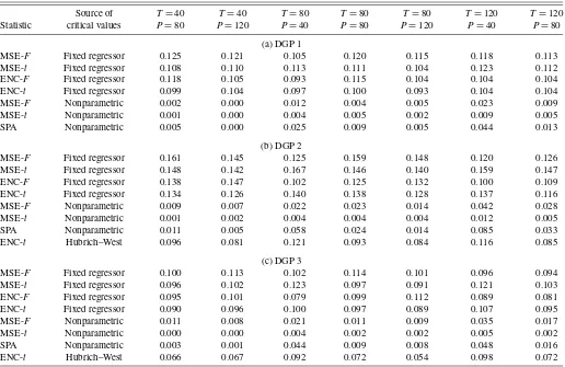
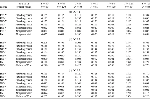
4.3 Size Results

The results presented in Tables 1 and 2 indicate that tests of equal MSE and forecast encompassing based on our pro-posed fixed regressor bootstrap have good size properties in a range of settings. For example, with DGPs 1 and 3, the empir-ical size of the MSE-ttest based on our bootstrap critical val-ues averages 10.8% (range, 9.1%–12.3%) at the one-step hori-zon and 11.3% (range, 9.6%–13.4%) at the four-step horihori-zon. In the same experiments, the empirical size of the ENC-ttest compared against fixed regressor bootstrap critical values av-erages 9.8% (range, 8.9%–10.7%) at the one-step horizon and 10.4% (range, 8.9%–12.3%) at the four-step horizon. In most (although not all) cases, the tests of forecast encompassing are of slightly snaller size than tests of equal MSE. In broad terms, theF- andt-type tests are of comparable size.

With DGP 2, the tests compared against critical values from our proposed bootstrap are prone to modest oversizing. For ex-ample, in these experiments, the size of the MSE-t test aver-ages 15.0% (range, 14.0%–16.7%) at the one-step horizon and 17.0% (range, 14.7%–18.8%) at the four-step horizon. In these DGP 2 experiments, the rejection rate for the ENC-ttest aver-ages 13.1% (range, 11.6%–14.0%) at the one-step horizon and 15.5% (range, 13.7%–16.8%), at the four-step horizon. As these examples indicate, with DGP 2, the oversizing is a little greater at the four-step horizon than at the one-step horizon.

Tests of forecast encompassing (or equality of adjusted MSEs) based on the approach of Hubrich and West (2010) have reasonable size properties at the one-step horizon, but not at the four-step horizon. With DGP 3 and one-step-ahead forecasts, the size of the ENC-ttest compared against critical values ob-tained by simulating the maximum of normal random variables ranges from 5.4% to 9.8%. For mostT,Psettings with DGP 3, the Hubrich–West approximation yields a slightly to modestly undersized test, consistent with simulation results in Hubrich and West (2010). But with DGP 2 and one-step-ahead forecasts, the ENC-ttest compared against Hubrich–West critical values can be slightly undersized or slightly oversized, with a rejection rate ranging from 8.1% to 12.1%. At the four-step horizon, the Hubrich–West approach yields too high a rejection rate, espe-cially for smallP; for example, with DGP 3, the rejection rate ranges from 16.7% to 35.6 %. The clear tendency of improv-ing size with increasimprov-ing Psuggests that the oversizing is due to small-sample imprecision of the autocorrelation-consistent estimated variance of the normal random variables. We leave the question of whether better size could be obtained with an alternative HAC estimator for futrue research.

(9)

Table 1. Monte Carlo results on size, one-step horizon (nominal size=10%)

Source of T=40 T=40 T=80 T=80 T=80 T=120 T=120

Statistic critical values P=80 P=120 P=40 P=80 P=120 P=40 P=80

(a) DGP 1

MSE-F Fixed regressor 0.125 0.121 0.105 0.120 0.115 0.118 0.113

MSE-t Fixed regressor 0.108 0.110 0.113 0.111 0.104 0.123 0.112

ENC-F Fixed regressor 0.118 0.105 0.093 0.115 0.104 0.104 0.104

ENC-t Fixed regressor 0.099 0.104 0.097 0.100 0.093 0.104 0.104

MSE-F Nonparametric 0.002 0.000 0.012 0.004 0.005 0.023 0.009

MSE-t Nonparametric 0.001 0.000 0.004 0.005 0.002 0.009 0.005

SPA Nonparametric 0.005 0.000 0.025 0.009 0.005 0.044 0.013

(b) DGP 2

ENC-t Hubrich–West 0.096 0.081 0.121 0.093 0.084 0.116 0.085

(c) DGP 3

NOTE: The DGPs are defined in eqs. (5) and (8). In all of these experiments, the coefficientbin the DGPs is set to 0, such that, in population, all of the models are equally accurate. For each artificial dataset, forecasts ofyt+τ(whereτdenotes the forecast horizon) are formed recursively using estimates of the forecasting equations described in Section 4.2. These forecasts are then used to form the indicated test statistics, given in Section 2.2.TandPrefer to the number of in-sample observations and one-step-ahead forecasts, respectively. In each Monte Carlo replication, the simulated test statistics are compared with bootstrapped critical values, using a significance level of 10%. Sections 2.3 and 4.1 describe the bootstrap procedures. The number of Monte Carlo simulations is 2000; the number of bootstrap draws is 499.

The results in Tables 1 and 2 also indicate that tests of equal MSE based on critical values obtained from a nonparametric bootstrap are generally unreliable for the null of equal accu-racy at the population level. Rejection rates based on the non-parametric bootstrap are systematically too low. In particular, across all three DGPs and the two forecast horizons, the size of the MSE-ttest peaks at 1.2%. At the one-step horizon, the size of the MSE-F test is modestly better, peaking at 4.2%. At the four-step horizon, the MSE-Ftest based on the nonparametric bootstrap is generally undersized for DGPs 1 and 3 but ranges from modestly undersized to slightly oversized for DGP 2. Con-sistent with the results of Hansen (2005), the SPA test is slightly more accurately sized than the MSE-tbased on the nonparamet-ric bootstrap. The greatest improvement occurs at the smallest forecast sample size ofP=40. For example, with DGP 2 and one-step forecasts, the rejection rate of the SPA test is 8.5%, compared with 1.2% for the nonparametric version of the MSE-ttest. At the four-step horizon, the spike in the rejection rate at P=40 is large enough to make the SPA test oversized: for in-stance, with DGP 2, the rejection rates of the SPA and MSE-t tests are 34.8% and 0.4%, respectively. This spike that occurs with a small sample and a multistep horizon suggests that the problem rests in the autocorrelation-consistent variance that en-ters the test statistic.

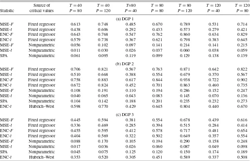
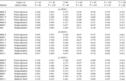
4.4 Power Results

The Monte Carlo results in Tables 3 and 4 on finite-sample power broadly reflect the size results. For testing the null of equal forecast accuracy at the population level, power is much better for tests based on our proposed fixed regressor bootstrap than for tests based on the nonparametric bootstrap. For a t -test of forecast encompassing, power based on the Hubrich– West approach to inference is similar to, although generally a bit lower than, power based on the fixed regressor bootstrap.

More specifically, based on critical values from the fixed re-gressor bootstrap, the powers of the MSE-F, MSE-t, ENC-F, and ENC-t tests are generally consistent with the patterns re-ported by Clark and McCracken (2001, 2005) for pairwise fore-cast comparisons. The empirical powers of these tests can be ranked as follows: ENC-F>MSE-F, ENC-t>MSE-t. MSE-Fis often more powerful than ENC-t, but the ranking of these two tests varies withτ and theT,Psetting. For example, with one-step- ahead forecasts, DGP 1, andT,P=80, 80, the pow-ers of the MSE-F, MSE-t, ENC-F, and ENC-ttests are 67.0%, 43.3%, 76.2%, and 62.1%, respectively. As might be expected, power increases with the size of the forecast sample; for in-stance, with one-step-ahead forecasts, DGP 1, andT=80, the rejection rate of the MSE-Ftest rises from 48.5% atP=40 to 78.9% atP=120.

(10)

Table 2. Monte Carlo results on size, four-step horizon (nominal size=10%)

(a) DGP 1

(b) DGP 2

(c) DGP 3

NOTE: See the note to Table 1.

At the one-step horizon, using the Hubrich and West (2010) approach to simulating critical values for the ENC-ttest yields modestly lower power compared with using the fixed regressor bootstrap. For example, in the DGP 3 results, the power of the ENC-ttest based on the fixed regressor bootstrap ranges from 32.2% to 64.9%, whereas power based on Hubrich–West criti-cal values ranges from 30.5% to 58.9%. However, at the four-step horizon, the Hubrich–West approach yields higher rejec-tion rates than the fixed regressor bootstrap method (for ENC-t), due to the size distortions of the Hubrich–West approach at the multistep horizon. For instance, with DGP 3 and τ =4, the power of the ENC-ttest based on the fixed regressor bootstrap ranges from 16.6% to 36.7%, whereas power based on Hubrich-West critical values ranges from 35.2% to 48.1%.

Rejection rates based on the nonparametric bootstrap are much lower. For the MSE-ttest, in most cases power is trivial, in the sense that it is below the nominal size of the test (10%). For example, under DGP 1, the rejection rate of the MSE-ttest ranges from 0.2% to 6.0% (across forecast horizons and sam-ple sizes). Power is quite a bit higher for the MSE-Fand SPA tests than for the MSE-ttest, but is still well below the power of the tests based on the fixed regressor bootstrap. For exam-ple, with one-step-ahead forecasts, DGP 1, andT,P=80, 80, the powers of the MSE-Fand SPA tests based on the nonpara-metric bootstrap are 21.4% and 12.9%, respectively, compared with the 6.0% power of the MSE-t test based on the nonpara-metric bootstrap. Using critical values from the fixed regressor

bootstrap raises the powers of the MSE-F and MSE-t tests to 67.0% and 43.3%. Although power based on the nonparametric bootstrap tends to be slightly to modestly higher with DGPs 2 and 3 than with DGP 1, the same patterns prevail.

5. APPLICATIONS

In this section we illustrate the use of the tests and inference approaches described earlier with two applications. In the first, based on the work of Chen, Rogoff, and Rossi (2010), we ex-amine the predictive content of exchange rates for commodity prices at a monthly frequency. In the second, patterned after such studies as that of Stock and Watson (2003), we apply our tests to forecasts of quarterly U.S. GDP growth based on a range of potential leading indicators.

More specifically, in the commodity price application, we ex-amine forecasts of monthly growth in commodity prices from a total of 28 models. Commodity prices are measured with the spot price for industrials published by the Commodities Re-search Bureau (CRB). The null model includes a constant and one lag of growth in commodity prices. The alternative mod-els add various combinations of a commodity futures price (the CRB index for industrial commodities) and exchange rates, all in growth rates and lagged 1 month (and with all exchange rates relative to the U.S. dollar). Drawing on the work of Chen, Ro-goff, and Rossi (2010), we use exchange rates for a few im-portant commodity economies with relatively long histories of

(11)

Table 3. Monte Carlo results on power, one-step horizon (nominal size=10%)

(a) DGP 1

(b) DGP 2

(c) DGP 3

NOTE: The DGPs are defined in eqs. (5) and (8). In all of these experiments, the coefficientbin the DGPs is set to the nonzero values given in Section 4.2, such that in population, the most accurate model is one of the alternatives. See the notes to Table 1.

floating exchange rates (Australia, Canada, and New Zealand), some other industrialized economies (U.K. and Japan), one in-dex of exchange rates for major U.S. trading partners, and an-other index of exchange rates for an-other important U.S. trading partners. To ensure some heterogeneity in predictive content, we have deliberately included some exchange rates (e.g., for Japan and the U.K.) that, based on the conceptual framework of Chen, Rogoff, and Rossi, should not be expected to have pre-dictive content for commodity prices.

The full set of variables and models for the commodity price application is listed in Table 5. The supplemental appendix pro-vides further descriptions of the data. Our model estimation sample begins with January 1987, and we examine recursive one-month-ahead forecasts for 1997 through 2008.

In the GDP application, we examine one-quarter-ahead and four-quarter-ahead forecasts of real GDP growth from 14 models. The null model includes a constant and one lag of GDP growth, where GDP growth is measured as (400/τ )ln(GDPt+τ/GDPt):

yt+τ=b0+b1yt+ut+τ. (11)

Each of 13 alternative models adds in one lag of a (potential) leading indicatorxt:

yt+τ=b0+b1yt+b2xt+ut+τ, (12)

where the set of leading indicators includes the change in con-sumption’s share in GDP (measured with nominal data), weekly

hours worked in manufacturing, building permits, purchasing manager indexes for supplier delivery times and orders, new claims for unemployment insurance, growth in real stock prices (real price=S&P 500 index/core PCE price index), change in 3-month Treasury bill rate, change in 1-year Treasury bond yield, change in year Treasury bond yield, 3-month to 10-year yield spread, 1-10-year to 10-10-year yield spread, and spread between Aaa and Baa corporate bond yields (from Moody’s). In supplemental results, we obtained very similar results using two lags of each leading indicator.

The complete set of variables and models for the GDP growth application is provided in Table 6. Further descriptions of the data are given in the supplemental appendix. Our model esti-mation sample begins with 1961:Q2, and we examine recursive forecasts for 1985:Q1+τ−1 through 2009:Q4.

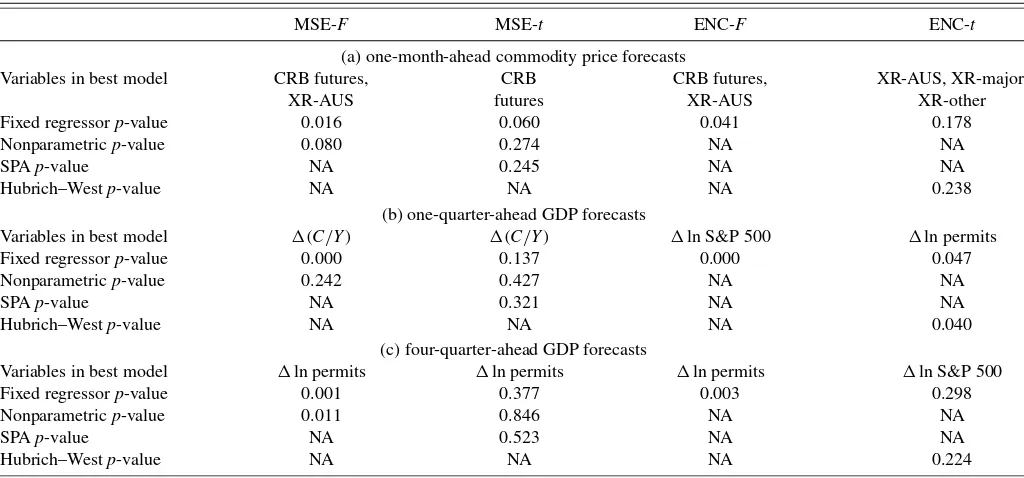
Tables 5–7 present the results of our applications. Tables 5 and 6 report root mean squared error (RMSE) ratios for each alternative model forecast relative to the benchmark (a num-ber<1 indicates that the alternative is more accurate than the benchmark) andp-values for tests of equal MSE and forecast encompassing, applied on a pairwise basis for each alternative compared with the benchmark. The models are listed in order of forecast accuracy (most to least accurate relative to the bench-mark model) as measured by RMSE. Table 7 providesp-values of the reality check tests, along with a listing of the best model identified by each test. We use 9999 replications in computing the bootstrapp-values.

(12)

Table 4. Monte Carlo results on power, four-step horizon (nominal size=10%)

(a) DGP 1

(b) DGP 2

(c) DGP 3

NOTE: The DGPs are defined in eqs. (5) and (8). In all of these experiments, the coefficientbin the DGPs is set to the nonzero values given in Section 4.2, such that in population, the most accurate model is one of the alternatives. See the notes to Table 1.

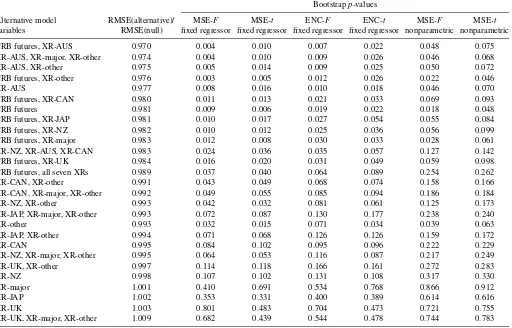
The pairwise forecast comparisons given in Table 5 indi-cate that both exchange rates and the commodity futures price have predictive content for spot commodity prices. Nearly all of the alternative models forecast commodity prices more accurately—although only slightly so, in terms of RMSEs— than the benchmark AR(1). The model with the lowest RMSE includes the constant and commodity price lag of the bench-mark model, the futures price, and the Australian dollar ex-change rate. Ranked by RMSE, the next few models include various combinations of the futures price, Australian dollar ex-change rate, major country exex-change rate index, and other im-portant trading partners exchange rate index. According to the pairwise tests based on the fixed regressor bootstrap, more than one-half of the models are significantly better than the bench-mark at the 10% significance level. Consistent with our Monte Carlo evidence, using a nonparametric bootstrap consistently yields higherp-values and implies fewer models with predic-tive content on a pairwise basis.

The reality check results provided in Table 7 show that, tak-ing the search for a best model into account, most of the tests compared against our proposed bootstrap critical values con-tinue to reject the null of equal forecast accuracy. In particu-lar, the lowest-MSE model remains significantly better than the benchmark; the reality check version of the MSE-F test has a fixed regressor bootstrapp-value of 1.6%, whereas the reality check version of the ENC-F test identifies the same model as

best and rejects equal accuracy with ap-value of 4.1%. Thet -tests for equal MSE and encompassing identify other models as best, with the reality check version of the MSE-ttest indicating that the model with the futures price is significantly more accu-rate than the benchmark, but the ENC-ttest failing to reject the null of equal accuracy. Again, consistent with the Monte Carlo results,p-values are considerably higher with the nonparamet-ric bootstrap than with our fixed regressor approach. Under the nonparametric approach to the reality check, neither MSE-tnor SPA rejects the null of equal accuracy.

The pairwise forecast comparisons presented in Table 6 show that at the one-quarter horizon, a handful of variables have sig-nificant predictive content for real GDP growth, whereas evi-dence of predictive content is much weaker at the four-quarter horizon. At the shorter horizon, most of the tests based on a fixed regressor bootstrap indicate that five models—those including (in addition to the constant and GDP growth lag of the benchmark), respectively, the change in the consump-tion share, growth in building permits, growth in stock prices, Baa−Aaa interest rate spread, and purchasing manager in-dex of new orders—forecast significantly better than the AR(1) benchmark (using a 10% significance level). As expected, p -values based on the nonparametric bootstrap are considerably higher and yield weaker evidence of predictive content, with both the MSE-Fand MSE-ttests rejecting the null for just the model including the change in the consumption share.

(13)

Table 5. Pairwise tests of equal accuracy for monthly commodity prices (one-month forecast horizon)

Bootstrapp-values

Alternative model RMSE(alternative)/ MSE-F MSE-t ENC-F ENC-t MSE-F MSE-t

variables RMSE(null) fixed regressor fixed regressor fixed regressor fixed regressor nonparametric nonparametric

CRB futures, XR-AUS 0.970 0.004 0.010 0.007 0.022 0.048 0.075 XR-AUS, XR-major, XR-other 0.974 0.004 0.010 0.009 0.026 0.046 0.068

XR-AUS, XR-other 0.975 0.005 0.014 0.009 0.025 0.050 0.072

CRB futures, XR-other 0.976 0.003 0.005 0.012 0.026 0.022 0.046

XR-AUS 0.977 0.008 0.016 0.010 0.018 0.046 0.070

CRB futures, XR-CAN 0.980 0.011 0.013 0.021 0.033 0.069 0.093

CRB futures 0.981 0.009 0.006 0.019 0.022 0.018 0.048

CRB futures, XR-JAP 0.981 0.010 0.017 0.027 0.054 0.055 0.084

CRB futures, XR-NZ 0.982 0.010 0.012 0.025 0.036 0.056 0.099

CRB futures, XR-major 0.983 0.012 0.008 0.030 0.033 0.028 0.061 XR-NZ, XR-AUS, XR-CAN 0.983 0.024 0.036 0.035 0.057 0.127 0.142

CRB futures, XR-UK 0.984 0.016 0.020 0.031 0.049 0.059 0.098

CRB futures, all seven XRs 0.989 0.037 0.040 0.064 0.089 0.254 0.262

XR-CAN, XR-other 0.991 0.043 0.049 0.068 0.074 0.158 0.166

XR-CAN, XR-major, XR-other 0.992 0.049 0.055 0.085 0.094 0.186 0.184

XR-NZ, XR-other 0.993 0.042 0.032 0.081 0.061 0.125 0.173

XR-JAP, XR-major, XR-other 0.993 0.072 0.087 0.130 0.177 0.238 0.240

XR-other 0.993 0.032 0.015 0.071 0.034 0.039 0.063

XR-JAP, XR-other 0.994 0.071 0.068 0.126 0.126 0.159 0.172

XR-CAN 0.995 0.084 0.102 0.095 0.096 0.222 0.229

XR-NZ, XR-major, XR-other 0.995 0.064 0.053 0.116 0.087 0.217 0.249

XR-UK, XR-other 0.997 0.114 0.118 0.166 0.161 0.272 0.283

XR-NZ 0.998 0.107 0.102 0.131 0.108 0.317 0.330

XR-major 1.001 0.410 0.691 0.534 0.768 0.866 0.912

XR-JAP 1.002 0.353 0.331 0.400 0.389 0.614 0.616

XR-UK 1.003 0.801 0.483 0.704 0.473 0.721 0.755

XR-UK, XR-major, XR-other 1.009 0.682 0.439 0.544 0.478 0.744 0.783

NOTE: As described in Section 5, monthly forecasts of the growth rate of commodity prices in periodt+1 are generated from a null model that includes a constant and growth in prices in periodtand alternative models that include the baseline model variables and the periodtvalues of the growth rates of the futures price and various exchange rates. The table lists the additional variables included in each alternative model. Forecasts from January 1997 to December 2008 are obtained from models estimated with a data sample starting in January 1987. This table provides pairwise tests of equal forecast accuracy. For each alternative model, the table reports the ratio of the alternative model’s RMSE to the null model’s forecast RMSE and bootstrappedp-values for the null hypothesis of equal accuracy for the test statistics indicated in the columns. Sections 2.3 and 4.1 describe the bootstrap procedures. The RMSE of the null model is 2.408; the predictand is defined as 100 times the log change in the price level.

At the longer horizon, only three models have RMSEs lower than the benchmark, and only one—the model including growth in building permits—is significantly better according to the pairwise tests. However, the ENC-Fand ENC-t tests indicate that at the population level, stock prices have significant pre-dictive content for GDP growth, even though in this sample the model yields an RMSE equal to that of the benchmark model. The ENC-Ftest yields the same result for the purchasing man-ager index of new orders.

The reality check test results provided in Table 7 show that some of the evidence of predictive content in leading indica-tors for GDP growth hold up (using fixed regressor bootstrap p-values) once the search for a best model is taken into account. As should be expected, thep-values are generally higher for re-ality check tests than pairwise tests. But the significance in the pairwise case mainly holds up under the reality check micro-scope. In particular, at the one-quarter horizon, the MSE-Ftest continues to indicate that the consumption share significantly improves forecasts of GDP growth—using fixed regressor crit-ical values, but not nonparametric critcrit-ical values. At the four-quarter horizon, the reality checkp-values of the MSE-F and ENC-Ftests are 0.1% and 0.3%, respectively, indicating build-ing permits have significant predictive content for GDP growth even when model search is taken into account. However, the

re-ality checkp-values for MSE-tand ENC-ttests (which gener-ally have lower power than theirF-type counterparts, according to our Monte Carlo results) are above the 10% threshold, failing to reject the null.

6. CONCLUSION

This article has developed a new bootstrap method for simu-lating asymptotic critical values for tests of equal forecast accu-racy and encompassing among many nested models. The boot-strap, which combines elements of fixed regressor and wild bootstrap methods, is simple to use. We first derive the asymp-totic distributions of tests of equal forecast accuracy and en-compassing applied to forecasts from multiple models that nest the benchmark model—that is, reality check tests applied to nested models. These distributions are nonstandard and involve unknown nuisance parameters. We then prove the validity of the bootstrap for simulating critical values from these distributions. Using our new fixed regressor bootstrap, we then conduct a range of Monte Carlo simulations to examine the finite-sample properties of the tests. These experiments indicate that our pro-posed bootstrap has good size and power properties, especially compared with the nonparametric methods of White (2000) and Hansen (2005) developed for use with nonnested models. In the