BIODIVERSITY DIFFERENT AND SPECIES ASSEMBLAGES OF PHYTOPLANKTON WITHIN OOZE SEDIMENT AT MYLL LAKES, NEW SOUTH WALES AUSTRALIA
Nita Rukminasari
Fakultas Ilmu Kelautan dan Perikanan Universitas Hasanudin
Jl. Perintis Kemerdekaan Km. 10, Tamalanrea, Makassar 90245, Sulawesi Selatan E-mail: [email protected]
Abstract
Phytoplanktons are primary producer, which determine the waters productivity. The assemblages of phytoplankton in the lake varied spatially and temporally as a result of nutrient concentration, some physical and chemical factors. However, the assemblage of phytoplankton in the lake were not well documented. The overall aims of the study wereto count and identify phytoplankton taxa and to examine assemblages at location with and without ooze, and to relate the presence/absence of ooze to phytoplankton abundance and assemblages. The samples were collected from Myall Lakes, NSW Australia. The data were analysed using multivariate analysis to determine assemblages of phytoplankton amongst location. Further more, univariate analysis was used to examine how the water quality was in particular presence/absence of ooze affected to phytoplankton abundance. The hypothesis being tested were: (1) phytoplankton assemblages vary spatially in
Myall Lake due to varying water quality characteristics, including presence of ooze, (2) there was a signiicant
difference of phytoplankton abundances between locations due to presence/absence of ooze.
In both instance the hypothesis on this study was accepted. There was a signiicant different not only
phytoplankton assemblages but also phytoplankton abundance within locations. It concluded that the phytoplankton varied spatially in those locations. Presence or absence of ooze affects abundance of phytoplankton. However, further study was needed to conduct in particular to determine certain aspects which affect the assemblages and abundances of phytoplankton.
Key words: biodiversity, myall lakes, ooze sediment, species assemblages Introduction
Phytoplankton is a primary producer of organic matter in the aquatic habitat. It has an important role in the aquatic food web. Phytoplanktons are predominantly autotrophic and are the primary producers of organic matter in aquatic ecosystem (Boney, 1975). Consequently, phytoplanktons determine productivity of aquatic habitat. Productivity of waters was determined by abundance and biomass of phytoplankton as a result of phytoplankton growth and composition. Sze (1998) stated that the growth of planktonic population depends on the rate at which new cells are produced in the photic zone and the rate of which cells are lost. Furthermore, net primary production by phytoplankton occurring is mainly dependent on the balance between gross photosynthesis and respiration, which will determine the critical depth (Kromkapm & Peene, 1995).
The major of phytoplankton species is a member of algae. Boney (1979) stated that members of the phytoplankton are classed as algae. Moreover, there is a particular characteristic of phytoplankton, such as moves
passively, loating in the water and has a microscopic
size (Boney, 1975 ; Sze, 1998; Graham, 1999).
Phytoplankton has a different assemblage. These assemblages are affected by physical, chemical and biological factor. Physically, the assemblage of phytoplankton is affected by depth, light, season, tide and temperature. Sze (1998) stated that the explanation proposed for the diversity of phytoplankton assemblages must include; (1) less time for the better competitors to eliminate the poorer competitors (2) selective grazing on potentially dominant species, (3) different nutrients or other resources limiting different species; and (4) patchy distribution of
phytoplankton population relate to insuficient time
gives rise to changing environmental condition or frequent disturbances, therefore poorer competitors are not eliminated. From selective grazing potentially dominant species are prevailed from becoming abundant to displace other species. The distribution of the phytoplankton population is separated into microhabitats and the apparent occurrence of many species occurring together is evident from mixing patches during sampling.
also found that plankton communities are structured by the simultaneous impact of bottom up (limitation by sources) and top down (control by predators) effect. Furthermore, Muylaert & Sabbe (1999) stated that community structure of phytoplankton might determine
the coniguration of food webs and the relative and
absolute importance of different trophic links. Mulyaert
et al. (2000) stated that variation in phytoplankton community as a whole and its relation to changes in the abiotic environment. They also stated that spatial variation of phytoplankton in the lake can attributed to differences in species composition between upper and lower freshwater tidal estuarine stations. In the upper reaches of the freshwater tidal estuary, the phytoplankton community was mainly of riverine origins. On the other hand, in the lower reaches of the freshwater tidal estuary, this riverine phytoplankton disappeared and is replaced by autochthonous population. Moreover, the biological factors that affect to phytoplankton assemblages are grazing. Hansen
et al. (1997) found that phytoplankton predominantly made up by cryptophytes were grazed in August to October. However, the cryptophytes showed negative responses to Daphnia grazing. Finally, the assemblages of phytoplankton is affected by chemical factor, such as salinity, dissolve oxygen, pH and nutrient level. Reynols (1998) stated that in lakes where the phosphorus concentration is always substantially below 1–2 µ gP/l, the phytoplankton is likely to tend quickly towards dominance by
high-afinity species.
There is a problem relates to phytoplankton assemblages, which is dominated species. When the phytoplankton is dominated by a certain species, for example blue green algae, this condition will give adverse effect to other organism, such as zooplankton,
ish, if the blue green algae is very abundant (bloom),
because the blue green algae has poison for other organism and inedible.
The assemblages of phytoplankton in the lake varied spatially and temporally as a result of nutrient concentration, some physical and chemical factors. Seasonally, the assemblage of phytoplankton is dominated by a particular species.
The assemblage of phytoplankton in the lake is not well documented. So, it is important to know the assemblages of phytoplankton in the lake. This study has two aims, namely: (1) to count and identify phytoplankton taxa and to examine assemblages at location with and without ooze (girtja), (2) to relate the presence/absence of ooze to phytoplankton abundance
and assemblages. Moreover, the hypothesis will be tested was: phytoplankton assemblages vary spatially in Myall Lake due to varying water quality characteristics, including presence of ooze.
Materials and Methods Study Site
The Myall lake is located on the Central Coast of New South Wales (32o26’S, 152o24’E) some 280 km north of Sydney and comprise the Broadwater, Boomlambayte lake and Myall lake (Atkinson, et al.,
1981). They are an interconnected series of shallow brackish lagoons, which drain via the Lower Myall River into Port Stephens at Tea Gardens. The lakes cover an area of approximately 11000 hectares and are generally 3.7–4 m deep with the Myall River reaching 8 m in depth (Atkinson et al., 1981).
Median annual rainfall for Bulahdelah was 1351 mm with 50% of all years having between 1136 mm and 1518 mm the wettest months were in late summer and early autumn with median monthly rainfalls exceeding 100 mm. The driest months were late winter and early spring with median monthly rainfalls of about 60 mm (Atkinson et al., 1981).
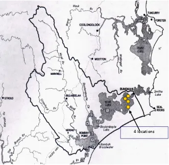
The study was conducted at Myall lake (Figure 1). It was consist of four location, which was two location with presence of ooze and two other location without ooze. Each location consisted of two different sites and at each site three samples was taken. In this study used a pole-integrated sampler.
Measurement of Variable
This study measured three main variables/parameters. Firstly, it was physical variable, namely: temperature, depth, turbidity and conductivity. Each method of physical variable is shown in Table 1. Secondly, the parameter was measured in this study was chemical factor, such as: salinity, dissolve Oxygen and pH. Device and method of this parameter is shown in Table 1. Thirdly, the study measured nutrient content, such as: Ammonia, Nitrite, Nitrate, Phosphate, and Silicate. This parameter was measured using spectrophotometer. Fourthly, the study counted and
identiied phytoplankton assemblage and abundant.
This parameter was determined by using Lugol’s method and Lund cell counting.
Identifying and Counting Phytoplankton
phytoplankton was preserved using Lugol’s dilution. There was two steps before phytoplankton was
identiied and counted. Firstly, phytoplankton was
sedimented using cylindries tube with 100 ml volume for at least 24 hours in the dark room. Secondly, making phytoplankton sample from the phytoplankton sedimented through taking 10 ml from total volume of phytoplankton sedimented.
Phytoplankton was counted using Lund Cell method. The Lund Cell has to be calibrated before it was used. The calibration of Lund Cell through determines the volume of each chamber by weighing it before and after
illing with deionised water. This weighing was repeated
[image:3.595.149.480.86.410.2]10 times and calculating the mean. The area of the chamber was calculated by multiplying the length of the cover slip by the distance between the two side pieces Figure 1. The map of study site, an arrow showing sampling station.
Table 1. Physical and chemical measurement method.
Parameter/Variable Physical/
Chemical Method Device
Temperature Physical In situ Water quality meter Yeo-Kal Transparancy Physical In situ Water quality meter Yeo-Kal Turbidity Physical In situ Water quality meter Yeo-Kal Conductivity Physical In situ Water quality meter Yeo-kal Salinity Chemical In situ Water quality meter Yeo-Kal Dissolve Oxygen Chemical In situ Water quality meter Yeo-Kal
PH Chemical In situ Water quality meter Yeo-Kal
Ammonia Chemical Laboratory Spectrophotometer
Nitrite Chemical Laboratory Spectrophotometer
Nitrate Chemical Laboratory Spectrophotometer
Phosphate Chemical Laboratory Spectrophotometer Silicate Chemical Laboratory Spectrophotometer Chlorophyll content Chemical Laboratory Spectrophotometer
[image:3.595.120.471.458.641.2]of Lund Cell. These lengths was measured either with the vernier scale. The area of Whipple graticule at each
magniication under the microscope was measured
using a stage micrometer.
Based on Hotzel & Croome (1999) the total number
of Whipple graticule ields within the total chamber
area was calculated as:
Total area of chamber (mm2) Total number of ield =
Area of Whipple graticule (mm2) The conversion factor for counting ields of view was
calculated as:
Field Factor (Ff) = 1/Lund Cell volume (ml) x total
number of ields.
The conversion factor (Ft) for counting short tranverses was calculated as :
Ft = Ff / (cell/Whipple graticule length)
The total tranverses in this phytoplankton counting was 7.
Total number of cell per ml was calculated using formula bellow :
C(cell/ml) = N/F x Ff
Where
N = number of cells or units counted
F = number of ields counted Ff = ield conversion factor
Statistical Analysis
Multivariate analysis
The assemblages of phytoplankton was analysed using PRIMER V.5 (Plymouth Marine Laboratories, UK) software program with standardised data and transformed to the fourth root and a Bray-Curtis similarity matrix was created. From this, non-metric multi dimensional scaling (nMDS) plots were constructed and one-way analysis of similarities (ANOSIM) conducted on the data set to compare the phytoplankton assemblages in term of the total number of cell/ml for each organism and the species composition. Pairwise test was used to determine which location assemblages were different from one another. To determine the dominant species and similarity assemblages of phytoplankton at each location, SIMPER analysis was run automatically in PRIMER software program.
Univariate analysis
Determination how was the water quality in particular presence/absence of ooze affected to phytoplankton abundance, the data was analysed by ANOVA method using the Gmav program. Factor included location,
which was orthogonal and ixed, and site which was
an nested and random factor. SNK test were used to
determine which treatment means were signiicant
from one another. All analysis was conducted at a
5% signiicance level.
Results and Discussion Multivariate Analysis
nMDS plot
Based on the nMDS plot showed clearly that there were difference assemblages of phytoplankton species and class within location (Figure 2a). The phytoplankton assemblages seem to separate from one –another. Interestingly, the species assemblages in location C and D (without ooze location) seem to close each other. However, the species assemblages between A and B was far to each other. The stress value of this plot was good enough to explain the similarity between species within location. Furthermore, there was no segregated of phytoplankton class within location. The pattern of class assemblages tended to close each other (Figure 2b).
Analysis of similarity
There was a signiicant different between location
in term of assemblages of species (ANOSIM, R=
0.448, P < 0.01). Not all location were signiicantly
different from one to another based on the pairwise test. A summary of this test can be seen in table
2. Meanwhile, There was a signiicant different of
phytoplankton class assemblages within location (ANOSIM, R = 0.608, P < 0.01). Moreover, pairwise
test showed that all location has a signiicantly different
of phytoplankton class assemblages (Table 3.)
Table 2. Summary of pairwise tests from ANOSIM comparing the species assemblages in term of total number of cell/ml.
Location A
Location B
Location
C Location D Location A - 0.167 0.374* 0.509**
Location B - - 0.794** 0.915**
Location C - - - -0.011
Location D - - -
[image:4.595.308.538.640.710.2]Table 3. Summary of pairwise tests from ANOSIM comparing the class assemblages in terms of total number of cell/ml.
Location A
Location B
Location C
Location D Location A - 0.613** 0.72** 0.613**
Location B - - 0.82** 0.874**
Location C - - - 0.265
Location D - - -
-Numbers are relevant Global R values , ** = signiicantly different (P < 0.01)
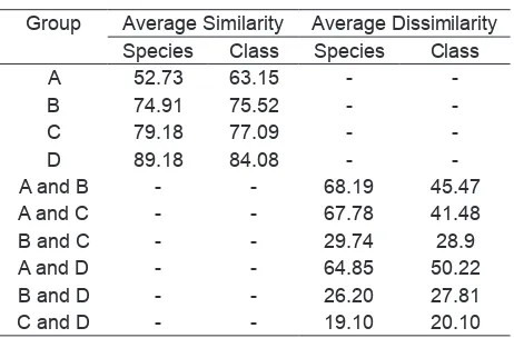
SIMPER
The SIMPER analysis showed that there was not only
a signiicant result for the average similarity within
group, but also average dissimilarity between groups, at species and class assemblages (Table 4).
Furthermore, each location was dominated by a particular species. Interestingly, all of location was dominated by the same class, such as Cyanophyceae.
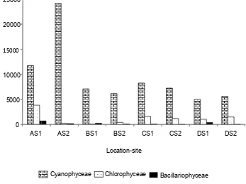
Univariate analysis results
The study found that there was a difference mean of abundance of total number of species (cell/ml) within location (Figure 3). The abundance of species was varied among the class of phytoplankton (Figure 4). As we can seen in the graph that location A site 2 (location with ooze) had a highest the average of total number of Cyanophyceae.
Statistically, there was a significant difference of species abundance between location with ooze and without ooze. SNK test determining that abundances of species at location with ooze was different from location without ooze. The statistical analyses, including ANOVA and SNK tests were summarised in table 5 and 6 respectively, for all variable.
Discussion
The study found that phytoplankton assemblage s e p a r a t e l y a m o n g s t l o c a t i o n . I n t e r e s t i n g l y, phytoplankton species in location C and D grouped closely each other. However, in location A and B the phytoplankton species was far away to each other.
This inding was indicated by the average of similarity
of species assemblages in those location. Location A and B has a lower average of similarity than location C and D. The difference of phytoplankton assemblages in those locations, presumed because of the difference of environmental condition between locations. Reynols (1998) indicated that a certain kind of community is more likely to be assembled than another, simply because particular environments influence the relative success of the individual organisms present. Furthermore, phytoplankton quantity, as well as its
species composition relects the trophic state of lake
(Lepisto & Rosentrom, 1998).
[image:5.595.309.540.306.458.2]Merismopedia was a dominated species in all of location. It assumed that the Myall lakes was more Figure 2. nMDS ordiantion of 4th root transformed non - standardised data comparing the phytoplankton species
(a) and class assemblages (b) in term of total number of cell/ml between location.
Table 4. Average similarity and dissimilarity (%) within groups at species and class assemblages.
Group Average Similarity Average Dissimilarity Species Class Species Class
A 52.73 63.15 -
-B 74.91 75.52 -
-C 79.18 77.09 -
-D 89.18 84.08 -
-A and B - - 68.19 45.47
A and C - - 67.78 41.48
B and C - - 29.74 28.9
A and D - - 64.85 50.22
B and D - - 26.20 27.81
C and D - - 19.10 20.10
A
B
C
D
Stress: 0.15 Stress: 0.16
Location
Copyright©2009. Jurnal Perikanan (Journal of Fisheries Sciences) All Right Reserved
[image:6.595.116.463.342.601.2]Figure 3. Mean and SE of phytoplankton abundance in each location and site.
[image:6.595.53.287.677.739.2]Figure 4. The average of cell number in three dominant class at location and both site.
Table 5. Summary of result from the ANOVA for the differences in means of abundances of species within location and site.
Sources df MS f P Value
Location 3 259477201.7 8.54 0.0326* Site (Lo) 4 30384324.1 0.78 0.5531 Residual 16 38844990.8
Total 23
*Signiicantly different (P < 0.05)
Table 6. Summary of SNK tests from the ANOVA comparing the abundance of species between location.
Location Signiicant different from A (with ooze) C and D
B (with ooze) Non signiicant from A,C and D C (without ooze) Non signiicant from B and D D (without ooze) A
40000
35000
30000
25000
20000
15000
10000
5000
0
Ph
yt
o
p
la
n
kt
o
n
a
b
u
n
d
a
n
ce
(C
e
ll/
ml
)
AS1 AS2 BS1 BS2 CS1 CS2 DS1 DS2
Location-Site
1
1
2 2
0 5000 0000
5000
20000 25000
AS1 AS2
Cyanophy
Figu BS1
Lo
Ch yceae
re 4 Hal 166 BS2 CS
ocation-site
lorophyceae
S1 CS2
Bacillario
DS1
ophyceae
acid, because this species usually dominate at acidophilic and was rare in lakes with phosphorus concentrations greater than 30 µg/l (Lepisto & Rosentrom, 1998). However, the data of water quality found that the pH in all of locations was around 7 – 9. There was an assumption to explain of contradicted
inding. It assumes that the phosphorous content in
the Myall Lake was high. DLWC (2001) found that the phosphorus loading to Myall Lakes was high, such as 0.117 mg/l of median total phosphorus concentration in Myall River. Consequently, the Merismopedia can grow well even though the pH of water was high.
Interestingly, Cyanophyceae was the most dominated class in all of location. There were some reasons to
explain the inding. Firstly, it was predicted that Myall lake
was eutrophic lake. DLWC (2001) found that substantial quantities of nitrogen (at least approximately 93 tonnes per annum) were delivered to the Myall Lakes system in annual discharge from the Myall River. Lepisto and Rosentrom argue that Cyanophyceae was the most important phytoplankton group in the eutrophic lake. Secondly, Cyanophyceae has a positive correlation to pH. This study found that pH value in all of location was relatively high, such as around 7–9. It provides a good condition for Cyanophycea species to grow. Temporenas, et al. (2000) indicated that Cyanophyceae biomass and pH were significantly correlated. It dominates at high pH, possibly due to the ability to use bicarbonate ion as a carbon source. Cyanobacteria have a distinct preference for netral to alkaline waters (Paerl, 1988). Thirdly, dominated Cyanophyceae in all location in this study was also assumed that those location was unbuffered waters condition. It was indicated by increasing pH value, as a consequent species with
eficient carbon-concentration mechanisms including
bloom-forming cyanobacteria (cyanophyceae) was occurred. Reynolds (1998) stated that in unbuffered waters (that is, relatively lacking of bicarbonate), rapid CO2 withdrawal by otherwise nutrients-replete algal growth leads to raised pH levels and to selective
weighting in favour of those species with eficient
carbon-concentrating mechanisms, including the bloom-forming cyanopbacteria. Fourth, cyanophyceae was dominated in all of locations, it predicted that those location has a wide range of environmental changes. Many cyanobacteria revealed a high degree of tolerance or a favorable response to excessive nutrient and/or pollutant loading,
signiicant accompanying shifts in total ionic strength or
salinity of affected waters can at times cause dramatic alterations in cyanobacteria dominance (Paerl, 1988). Finally, dominated cyanophyceae in all of locations
indicated that this class was governed assemblages of the species in the winter. Wiedner & Nixdorf (1998) found that the cyanobacteria was known to over winter in considerable densities, due to its ability to adapt to low –light, especially if winter growth is uninterrupted by long-term ice and snow-cover. Moreover, severe winters prevent the rise of cyanobacterial dominance, whereas mild winters support cyanobacterial overwintering and improve the inoculum for future dominant population (Wiedner & Nixdorf, 1998).
The study found that the mean of phytoplankton abundance was higher in location A at both sites than other location. Statistically, there was a significant different of phytoplankton abundance amongst location. SNK test showed that location A (with ooze) was different from location C and D (without ooze). On the other
hand, location B, C and D was no signiicant different
to each other. There is some assumption to explain this
inding. Firstly, it predicted that location A had a higher
nutrient content that other location. Consequently, the phytoplankton in this location had a higher growth rate than other locations. Phytoplankton growth was nutrient limited, because the biomass of population living in nutrient depleted environments increases in response to nutrient enrichment (Hein & Reimann, 1996). Furthermore, location A had a lowest average of phytoplankton-class similarity than other location; it was assumed that location A was less mesotrophic than other location. Dasi et al. (1998) found that mesotrophic reservoirs showed a rather more homogeneous phytoplankton structure. Finally, location A has a highest number of cyanophyceae, it presumed that in location A had a high nitrogen content due to the ability of many
cyanobacteria ix the nitrogen. Sze (1997) stated that
many symbiotic of cyanobacteria fix nitrogen and
thus beneit their hosts as nitrogen sources as well as
photosynthetic producers.
Surprisingly, the study found that the mean of chlorophyll content was highest in location A (site 1), which was 3.57 µg/l. It assumed that in location A has a high diversity of species, high nutrient content and high light penetration. Temporenas et al. (2000) stated that chlorophyll a content of the algae in the studied lake seems to depend on species composition, nutrient availability and light condition.
Conclusions
Phytoplankton assemblages were spatially in Myall
lakes on September 2002. There were a signiicant
ooze. It assumed that amongst location has a different environmental condition in term of water quality. The species was dominated by Merismopedia in all of location. It predicted that there was a high content of phosphorous in those locations.
Cyanobacteria was a dominated class in all of location. Based on this finding can be assumed that : (1) Myall lake was eutrophic lake, (2) there was positive correlation between cyanophyceae and pH, (3) the location of study was unbuffered waters condition, (4) the locations had a high wide range of environmental changes, (5) cyanobacteria was governed of species assemblages in the winter.
Abundances of phytoplankton was differed signiicantly
within locations due to a difference of water quality and presence of ooze.
References
Atkinson, G. 1981. An ecological investigation of the Myall Lakes region. Australian Journal of Ecology.
6, p. 299–327.
Boney, A.D. 1975. Phytoplankton. Edward Arnold (Publisher) Limited. London.
Dasi, M.J., M.R. Miracle, A. Camacho, J.M. Soria & E. Vicente. 1998. Summer phytoplankton assemblages across trophic gradients in hard-water reservoirs. Hydrobiologia 369/370: 27–43.
Department of Land & Water Conservation. 2001. Myall Lakes catchment data collation report, NSW Department of Land and Water Conservation. New South Wales.
Graham, L.F. & L.W. Wilcox. 2000. Algae. Upper Saddler River: Prentice Hall: USA.
Hansen, A.M., F.S. Andersen & J.S. Jensen. 1997. Seasonal pattern in nutrient llimitation and grazing control of the phytoplankton community in a
non-stratiied lake. Freshwater Biology 37: 523 – 534.
Hein, M. & B. Reimann. 1995. Nutrient limitation of phytoplankton biomass or growth rate: an experimental approach using marine enclosures. Journal of Experimental Marine Biology and Ecology 188: 167–180.
Hotzel, G. & R. Croome. 1999. A phytoplankton methods manual for Australian freshwaters. Land and Water Resources. Canberra.
Kromkamp, J. & J. Peene. 1995. On the net growth of phytoplankton in two Dutch estuaries. Water Science Technology 32 (4): 55–58.
Lepisto, L. & U. Rosenstrom. 1998. The most typical phytoplankton taxa in four types of boreal lakes. Hydrobiologia 369/370: 89–97.
Muylaert, K. & K. Sabbe. 1999. Spring phytoplankton assemblages in and around the maximum turbidity zone of the estuaries of the Elbe (Germany), the Schelde (Belgium/The Nederlands) and the Gironde (France). Journal of Marine System 22: 133–149.
Muylaert, K., K. Sabbe & W. Vyverman. 2000. Spatial and temporal dynamics of phytoplankton communities in a freshwater tidal estuary (Schelde, Belgium). Estuarine, Coastal and Shelf Science 50: 673– 687.
Paerl, H.W. 1988. Growth and reproductive strategies of freshwater blue green algae (Cyanobacteria), in Sandgren, C.D (eds), Cambridge University Press: Cambridge.
Reynolds, C.S. 1998. What factors inluence the species
composition of phytoplankton in lakes of different trophic status?. Hydrobiologia 369/370: 11–26.
Rothhaupt, K.O. 2000. Plankton population dynamics: food web interaction and abiotic constraints. Freshwater Biology 45: 105–109.
Sze, P. 1998. A biology of the algae. WCB McGraw-Hill: USA.
Temponeras, M., J. Kristiansen & M. Moustaka-Gouni. 2000. Seasonal variation in phytoplankton composition and physical-chemical features of the shallow lake Doirani, Macedonia, Greece. Hydrobiologia 424:109–122.
Wiedner, C. & B. Nixdorf. 1988. Success of
chrysophycetes, cryptophytes, and dinolagellates