T H E J O U R N A L O F H U M A N R E S O U R C E S • 46 • 1
Behavior
Evidence from the Ports of Los Angeles
Enrico Moretti
Matthew Neidell
A B S T R A C T
A pervasive problem in estimating the costs of pollution is that optimizing individuals may compensate for increases in pollution by reducing their exposure, resulting in estimates that understate the full welfare costs. To account for this issue, measurement error, and environmental confounding, we estimate the health effects of ozone using daily boat traffic at the port of Los Angeles as an instrumental variable for ozone. We estimate that ozone causes at least $44 million in annual costs in Los Angeles from res-piratory related hospitalizations alone and that the cost of avoidance be-havior is at least $11 million per year.
I. Introduction
Air pollution has long been recognized as a negative externality, but considerable debates have ensued over the optimal level of air quality, with few more contentious than the one surrounding ozone.1Ozone is presumed to have del-eterious effect on health, especially for children, the elderly, and those with existing respiratory illnesses, but the exact magnitude is disputed. Part of this controversy stems from discrepancies over statistical approaches to estimate the health effects of ozone and its associated costs on society.
1. A proposed ozone standard issued by the EPA in 1997 was finally upheld by the Supreme Court in 2002, but only after endless appeals and lengthy lawsuits initiated by states and industry (Bergman 2004). Furthermore, since higher temperatures favor ozone formation, climate change is expected to increase ozone levels (Racherla and Adams 2009), making regulations surrounding ozone an area of increasing importance. Enrico Moretti is a professor of economics at the University of California, Berkeley. Matthew Neidell is an assistant professor of health policy and management at Columbia University. Some of the data used in this article are available from August 2011 through July 2014, while information on obtaining the confidential data will be provided upon request from Matthew Neidell, Columbia University, 600 W. 168th Street, 6th floor, New York, NY 10032, mn2191@columbia.edu.
[Submitted April 2009; accepted October 2009]
Estimating this relationship is complicated for several reasons. First, a pervasive problem in the literature on the costs of pollution is that optimizing individuals may compensate for increases in pollution by reducing their exposure to protect their health. Behavioral responses to ozone levels are unlikely to be trivial because daily pollution forecasts are widely available through television and newspapers. Because ozone rapidly breaks down indoors, at-risk individuals can easily reduce short-run exposure by going indoors. Indeed, Neidell (2009) shows that air quality warnings reduce time spent outdoors. Therefore, even if one could isolate random variation in pollution, estimates that do not account for these behavioral responses will understate the full welfare effects of ozone. This is particularly relevant be-cause individuals most at risk have the greatest incentive to adopt compensatory behavior.2
A second challenge in estimating the costs of pollution is confounding from en-vironmental factors that may bias standard estimates. For example, weather directly affects health (for example, see Deschenes and Moretti 2009) but also affects ozone levels. Although some measures of weather conditions are observable and can in principle be controlled for, it is difficult to fully control for all weather factors with the correct functional form. Recent evidence by Knittel, Miller, and Sanders (2009) demonstrates that adding higher order terms for temperature and precipitation and adding second order polynomials for wind speed, humidity, and cloud cover has considerable impacts on estimates of health effects from pollution levels. It is even more difficult to control for allergens, which are related to both asthma and pollution, at a sufficient spatial and temporal level.3Given that the strong daily variations in pollution are unlikely to be driven solely by anthropogenic sources, it is crucial to properly account for the wide range of environmental factors that vary at a daily level.
A third challenge in estimating the cost of pollution arises from measurement error in assigning pollution exposure to individuals. The most common approach for measuring exposure is to assign data from ambient air pollution monitors to the residential location of the individual using various interpolation techniques. Given the tremendous spatial variation in pollution within finely defined areas (Lin, Yuong, and Wang 2001), this approach is likely to yield considerable measurement error. In fact, Lleras-Muney (2009) finds estimates are quite sensitive to the interpolation technique used.4
2. Although Neidell (2009) finds support for the existence of avoidance behavior, by controlling for only one source of avoidance behavior the estimates are not necessarily informative on the overall magnitude of avoidance behavior and its ultimate impact on the estimated costs of pollution. It is likely that there are several additional sources of information that at risk individuals use to adjust their behavior. Furthermore, in Neidell (2009) these pieces of information may be measured with error since they are assigned at a broader level than are observed pollution levels.
3. For example, Hiltermann et al. (1997) find a correlation of 0.57 between ozone and mugwort pollen, a pollen demonstrated to cause airway inflammation in asthmatics.
In this paper, we seek to identify the short-run effects of ozone on health ac-counting for avoidance behavior, confounding factors, and measurement error, and to provide estimates of the welfare effects and costs of avoidance behavior from ozone-related hospitalizations in the Los Angeles area. To address the three meth-odological challenges described above, we use daily data on boat arrivals and de-partures into the port of Los Angeles as an instrumental variable for ozone levels. Three features make boat traffic an appealing instrument. First, boat traffic represents a major source of pollution for the Los Angeles region. The combined ports of Los Angeles and Long Beach, the largest in the United States and third largest in the world, represent the single most polluting facility in the Los Angeles metropolitan area (Polakovic 2002). Because most of these boats come from countries with much less stringent environmental regulations, they contain less sophisticated emissions technology than their U.S. counterparts and emit unusually high levels of nitrogen dioxides (NOx)—contributing to over 20 percent of all NOx emissions in the Los Angeles area (AQMD 2002)—which gets carried inland to form ozone.5Our data confirm that boat traffic significantly affects daily ozone levels and, important for our identification, the effect of boat traffic on ozone levels declines monotonically with distance from the port.
Second, daily variation in boat traffic is arguably uncorrelated with other short-run determinants of health. The majority of boats arriving at the port travel from overseas. Several factors, such as the extended length of travel and unpredictable conditions at sea, make the exact date of arrival and departure difficult to predict. Therefore, the influx of pollution due to port activity is arguably a randomly deter-mined event uncorrelated with factors related to health, and we provide several pieces of information to support this.
Third, and crucially, boat traffic is generally unobserved by local residents. The arrivals and departures are not included in ozone forecasts or reported by newspapers and local news outlets. Indeed, we find that ozone forecasts and participation in outdoor activities are empirically orthogonal to boat traffic. Therefore, it is difficult for individuals to respond to ozone levels as affected by boat traffic, suggesting that our instrumental variable estimate holds compensatory behavior fixed.
While it is in theory possible that any difference between instrumental variable estimates and OLS estimates is due to the fact the former reflect a particular local average treatment effect (LATE)—namely, the impact of an increase in pollution due to port traffic on health—this possibility seems highly unlikely in our setting.6 The ozone created by emission from boats is chemically identical to the ozone created by emissions from other sources. Furthermore, ozone levels as affected by our instrument are quite comparable to the overall mean level of ozone at the port.7
5. In fact, emissions from the port have lead to numerous contentious debates, and a recent senate com-mittee hearing on port pollution lead by Senator Barbara Boxer from California seeks an urgent, national response to port pollution. Evidence of the passion behind the debate is succinctly summarized by the following quote from Bob Foster, mayor of Long Beach: “We’re not going to have kids in Long Beach contract asthma so someone in Kansas can get a cheaper television set.” (Wald 2007).
6. To the extent that the effects of ozone are nonlinear, then our results, whether from OLS or IV models, may not generalize to areas with sufficiently different ozone levels,
It is therefore plausible to think that heterogeneity in the ozone effect is limited in our setting.8
Our findings are striking. OLS estimates of ozone on hospitalizations are statis-tically significant but small in magnitude: Exposure to ozone causes $11.1 million per year in hospital costs in Los Angeles. In contrast, instrumental variable estimates indicate a significantly larger cost of ozone concentrations of about $44.5 million per year, with several robustness checks supporting our main findings. These esti-mates represent a lower bound of the total costs of ozone because it ignores health episodes that do not result in hospitalizations. Since for the marginal individual the marginal benefit of avoidance behavior must equal its marginal cost, under several additional assumptions we calculate that the overall cost of avoidance behavior must be at least $11.1 million per year in Los Angeles, noting that this does not include inframarginal individuals. More broadly, these results indicate the importance of accounting for several econometric factors in understanding the full welfare effects from pollution.
II. Background on Air Pollution and Health
Ground-level ozone is a criteria pollutant9regulated under the Clean Air Acts that affects respiratory morbidity by irritating lung airways, decreasing lung function, and increasing respiratory symptoms, with effects exacerbated for suscep-tible individuals, such as children, the elderly, and those with existing respiratory conditions like asthma. Symptoms can arise from contemporaneous exposure in as quickly as one hour of exposure. Because it may take time for exacerbation of respiratory illnesses, symptoms may arise from cumulative exposure over several days or several days after exposure. For example, “an asthmatic may be impacted by ozone on the first day of exposure, have further effects triggered on the second day, and then report to the emergency room for an asthmatic attack three days after exposure” (Environmental Protection Agency 2006). Thus it is necessary to control for several lags when estimating the relationship between ozone and health.
The process leading to ozone formation makes it highly predictable and straight-forward to avoid. Ozone is not directly emitted but forms from interactions between nitrogen oxides (NOx) and volatile organic compounds (VOC) in the presence of sunlight and heat. Therefore, ozone levels can be predicted fairly accurately using weather forecasts. Furthermore, ozone rapidly breaks down indoors where there are more surfaces to interact with (Chang et al. 2000). Since symptoms from ozone
decreased by one standard deviation (SD) from the mean (based on estimating our first stage equation). The adjusted mean for a one SD decrease in boat traffic is 0.0369 and a one SD increase is 0.0420. The unadjusted mean of ozone at the port is 0.0396, which is bounded by the two adjusted means, so the IV variation is at similar levels of ozone to the overall variation
8. Since our instrument is assumed to have a different effect on ozone depending on distance from the port, the above statement is true under the plausible assumption that effect of ozone on human health is the same for residents of Los Angeles who live close and far from the port.
exposure can arise over a short period of time, altering short-run exposure by going indoors can reduce the onset of symptoms.
Given the potential effectiveness of avoidance behavior, two forms of public in-formation are available to inform the public of expected air quality conditions: the pollutant standards index (PSI) and air quality episodes. The PSI, which is forecasted on a daily basis, is computed for five criteria pollutants, and the maximum PSI across pollutants is required by federal law to be reported in major newspapers along with a brief legend summarizing the health concerns (Environmental Protection Agency 1999). California state law requires the announcement of a Stage I air quality episode, or smog alert, when the PSI is at least 200, which corresponds to 0.20 parts per million (ppm) for ozone.10These episodes, which also occur on a daily basis, are more widely publicized than the PSI; they are announced on both television and radio.11
The agency that provides air quality forecasts and issues smog alerts for Southern California is the South Coast Air Quality Management District (SCAQMD). They produce the following day’s air quality forecast by noon the day before to provide enough time to disseminate the information. Because SCAQMD covers all of Orange County and the most populated parts of Los Angeles, Riverside, and San Bernardino counties—an area with considerable spatial variation in ozone—they provide the forecast for each of the 38 source receptor areas (SRAs) within SCAQMD. When an alert is issued, the staff at SCAQMD contacts a set list of recipients, including local schools and news media, who further circulate the information to the public.
Neidell (2009) provides direct evidence that people respond to information about air quality. He identifies the effect of smog alerts by using a regression discontinuity design that exploits the deterministic selection rule used for issuing alerts. When smog alerts are issued, attendance at major outdoor facilities in Los Angeles de-creases by as much as 13 percent.
III. Data
Our final data set consists of several different data sets merged to-gether at the daily level by zip code for the months April-October for the years 1993-2000 for all zip codes in SCAQMD. For health data, we use respiratory related emergency department (ED) visits from the California Hospital Discharge Data (CHDD) for the following age groups: 0-5, 6-14, 15-64, and older than 64.12There are two practical factors that make the CHDD an attractive option. First, it includes
10. Additionally, a Stage II air quality episode is issued when the PSI exceeds 250 or ozone forecast exceeds 0.30 ppm, but this only occurred once over the time period studied.
11. Although air quality episodes can potentially be issued for any criteria pollutant, they have only been issued for ozone. Because ozone is a major component of urban smog, this has given rise to the term “smog alerts.”
Table 1
Summary Statistics for Hospital Admissions, Ozone, and Covariates for Years 1993–2000
Mean Standard
deviation
A. Dependent variables (daily admissions)
Any respiratory illness 0.097 0.333
Age 0-5 0.043 0.216
Age 6-14 0.018 0.135
Age 15-64 0.129 0.376
Age 65Ⳮ 0.199 0.465
Pneumonia 0.037 0.199
Bronchitis/asthma 0.033 0.186
Other respiratory illness 0.027 0.167
B. Independent variables (five-day average)
Eight-hour ozone (ppm) 0.050 0.018
Eight -hour carbon monoxide (PSI) 16.60 9.04
One-hour nitrogen dioxide (PSI) 18.3 6.92
Maximum temperature (⬚F) 80.37 9.04
Minimum temperature (⬚F) 59.08 5.90
Precipitation (hundreths of inches) 1.02 4.63
Resultant wind speed (mph) 5.74 1.48
Maximum relative humidity (percent) 90.24 5.09
Average cloud cover sunrise to sunset (percent) 4.42 1.65
Boat traffic (tons / 1000) 514.49 55.58
N 1,927,187
the exact date of admission to the hospital and zip code of residence of the patient, enabling us to readily merge it to the other data. Second, it contains the entire universe of discharges and the primary diagnosis of the patient, providing a large sample for detecting respiratory related admissions at such a high frequency. Table 1 shows the daily number of ED respiratory illness admissions per zip code for the age groups considered, as well as the breakdown across types of respiratory illnesses and other independent variables used in this analysis.13
We use daily pollution data maintained by the California Air Resources Board. There are roughly 35 continuously operated ozone monitors and roughly 20 for carbon monoxide (CO) and nitrogen dioxide (NO2), two other pollutants necessary
to consider because of their correlation with ozone and potential health effects.14 We assign pollution levels to the SRA based on the values for the monitor in that SRA, and when no monitor is present, assign pollution values from the monitor in the nearest SRA.15
Data on boat traffic comes from the marine exchange of southern California. The marine exchange records daily logs of the arrival and departure dates of each indi-vidual vessel that enters the port, along with the net tons, length, flag, and cargo type of the vessel.16We aggregate this information to the total number of tons of boats arriving and departing on a daily basis. Using the latitude and longitude of the centroid of each zip code, we compute the physical distance from each zip code to the port.
Finally, data on weather is obtained from the Surface Summary of the Day (TD3200) from the National Climatic Data Center. Using the 30 weather stations available in SCAQMD, we assign daily maximum and minimum temperature, pre-cipitation, resultant wind speed, maximum relative humidity, and sun cover to each SRA in an analogous manner to pollution.17
IV. Conceptual Framework
To fix ideas on measuring and interpreting the effect of pollution on health, assume the following short-term health production function:
h⳱h(ozone,avoid,W,S) (1)
wherehis a measure of health,ozoneis ambient ozone levels, andavoidis avoidance behavior. W are other environmental factors that directly affect health, such as weather, allergens, and other pollutants.S are all other behavioral, socioeconomic, and genetic factors affecting health.
There are two main approaches to estimating Equation 1 and determining the welfare effects from changes in pollution, with the key difference arising in how avoidance behavior is treated. The first, and most common, is the dose-response
14. Particulate matter was not included in this analysis because measurements are not taken on a daily basis. We elaborate on the potential impact from omitting this variable below in the results section. 15. Given that this may induce measurement error, we also estimated models that limit the sample to only SRAs where an ozone monitor is present, but find no considerable difference in estimates. There are considerable disagreements over how to assign pollution from monitors to individuals. For example, as-signing pollution at a finer geographic level, such as the zip code, has potential to improve accuracy, but may also worsen it if people travel beyond their zip code. Using SRAs is justified on the grounds that SRAs were specifically designed to represent an area with common pollution concerns that account for geographic and population differences within SCAQMD, so there is a high degree of uniformity in ozone levels within an SRA.
approach, which does not control for avoidance behavior when estimating Equation 1 and thus obtains the total derivative of health with respect to ozone:dh/dozone ⳱␦h/␦ozoneⳭ␦h/␦avoid*␦avoid/␦ozone. Because engaging in avoidance behavior may result in welfare loss, in order to measure the full willingness to pay (WTP) for a reduction in pollution one must not only measure the loss associated withdh/ dozonebut also measure the costs associated with any changes in avoidance behavior (Cropper and Freeman 1991; Deschenes and Greenstone 2007). A common expres-sion for WTP using the dose-response approach is WTP⳱dh/dozone*(mⳭw)Ⳮ pavoid*␦avoid/␦ozone, wheremare medical expenditures incurred for any illness,w
is the value of lost time from the illness, andpavoidis the price of avoidance behavior (Harrington and Portney 1987).18
The second approach for estimating WTP directly accounts for avoidance behavior to estimate the partial derivate ␦h/␦ozone of the health production function, and measures the loss associated with the change in health:WTP⳱␦h/␦ozone*(mⳭw)
(Harrington and Portney 1987). Previous efforts using this approach attempt to di-rectly control for avoidance behavior in Equation 1 (Neidell 2004; Neidell 2009).19 Since both approaches require measuring changes in typically nonmarket behaviors, valuing the welfare effects from a change in environmental quality remains a pe-rennial challenge.20
Instead of directly observing avoidance behavior to estimate␦h/␦ozone, the strat-egy used in this paper is to use an instrument that shifts ozone levels but is unrelated to both avoidance behavior and other unobserved determinants of health.21As de-scribed in the introduction, we use boat traffic at the ports as an instrument for ozone levels to obtain estimates of␦h/␦ozone. Below we confirm a strong partial correlation between boat traffic and ozone levels and present evidence to support the assumption that boat traffic is uncorrelated with avoidance behavior and unobserved confound-ers. Moreover, because we have estimated the partial derivative␦h/␦ozone, we can estimate WTP using estimates of medical expenditures and the value of time and thus do not need to measure avoidance behavior.
Furthermore, if we obtain WTP estimates using the health production approach, then we also can obtain estimates of the costs of avoidance behavior. If we use OLS estimates to obtaindhealth/dozone, then we can obtain the first component of the dose-response WTP, commonly referred to as the cost of illness (COI). If we use the IV estimates to obtain ␦h/␦ozone, then we can obtain the full WTP. Therefore, the difference between WTP and COI ispavoid*␦avoid/␦ozone, which is the cost of
18. Note that our expression slightly differs from Harrington and Portney (1987) because we do not allow health to directly affect utility, but instead use all time lost from illness in place of only time lost in the workplace.
19. Instead of controlling directly for avoidance behavior, Neidell (2004, 2009) controls for factors that shift the demand for avoidance behavior (ozone forecasts and smog alerts). Note that the dose response and health production estimates are identical if avoidance behavior does not exist.
20. Another strand of literature uses stated-preference to elicit WTP; see, for example Alberini and Krup-nick (2000).
avoidance behavior. This simple yet remarkable result enables us to measure the costs of a typically nonmarket behavior without directly observing it.
V. Empirical Strategy
We estimate the following equations by two stage least squares:
h ⳱ ozone ⳭW ⳭMⳭ␣ ⳭⳭf(t)Ⳮu
(2) azst 1 st 2 st 3 t a z azst
ozone ⳱␥boatsⳭ␥ boats*distⳭ␥W Ⳮ␥MⳭⳭf(t)Ⳮv
(3) st 1 t 2 t s 3 st 4 t z st
where Equation 2 is the second-stage regression and Equation 3 is the first stage regression.hazstis the number of respiratory related ED admissions for age groupa
in zip code zof SRA sat date t. To remain consistent with previous ozone time-series studies that often found respiratory effects up to four days after exposure (Environmental Protection Agency 2006), we compute the daily average of ozone, boats, andWover the past five days.22We average across five days because we are only interested in testing whether an effect of ozone exists, and not the particular timing of the effect. Furthermore, a more flexible structure that allows each lag to enter separately would require us to instrument for each lag of ozone, which greatly reduces the precision of our estimates.23
The vector W includes maximum temperature, minimum temperature, precipita-tion, resultant wind speed, humidity, sun cover, carbon monoxide, and nitrogen di-oxide.Mtcontains day of week dummies to account for within week patterns of air quality and health. In addition to limiting the analysis to the months of April through October,f(t)includes year*month dummy variables and a cubic time trend to flexibly capture seasonality and long-run trends in air quality and health.24␣
aare age dummy
variables.zare zip code fixed effects designed to capture local time-invariant dem-ographic factors that might affect health as well as time-invariant measurement er-ror.25 uis an error term that includes avoidance behavior, unobserved components ofWandS, and an idiosyncratic component.
We instrument ozone in Equation 2 using boat traffic, shown in Equation 3.boatst
is a measure of tons of boat arrivals and departures at datetanddistsis the distance
from SRA sto the port. We interact boatstwith distance to allow the effect of the
22. We also estimated models that included four- or six-day averages of all variables, and this had minimal impact on our estimates.
23. We also estimated models with contemporaneous and the four lags of both pollution and weather entered separately, and the individual coefficients on ozone were all statistically insignificant. The sum of the ozone coefficients, which has the same interpretation as our five-day average, was 0.441, which is quite comparable to estimates using our five-day average.
24. We also estimated models with year*week dummy variables and found this had little impact on our estimates.
boat arrivals and departure to vary depending on how far the SRA is from the port. In all the empirical models in the paper, we cluster all standard errors by date.26
If there is a homogeneous effect of ozone on health, a necessary assumption for unbiased estimates of1is that cov(boatst, uazst)⳱0and cov(boatst*dists, uazst)⳱0.
Several factors support the validity of this assumption. One, the supply of commod-ities is a stochastic process such that variation in the production of goods and ser-vices and their loading and unloading at the port cannot be timed perfectly. For instance, on any given day the port averages approximately 15 boat arrivals, but the interquartile range of 12 to 17 suggests considerable variation in the number of arrivals. Two, although one vessel is docked at each berth at the port, there is substantial variation in the tonnage of these boats, an important factor affecting emissions, particularly NOx (Environmental Protection Agency 2000; Gajendran and Clark 2003). In support of this, the average boat tonnage is roughly 17,000, but the interquartile range is from 9,300 to 22,000. Three, given that these boats travel from great distances, conditions at sea and vessel travel speeds are likely to affect their exact arrival date.27These factors suggest it is reasonable to think of the timing of boat arrivals as virtually random in the short-run. Because of that, we have little reason to expect that short-run variations in boat movements directly affect health in the short-run, and below we present supporting evidence.
VI. Results
A. Validity of Boat Traffic as an Instrument
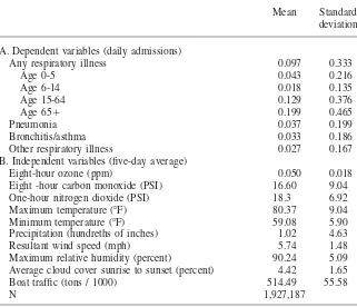
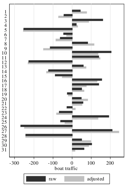
To support the validity of our instrument, we begin by demonstrating the virtually random day-to-day fluctuations in boat traffic. In Figure 1, we plot daily boat traffic for July, 2000, both unadjusted and adjusted for all covariates used in the analysis.28 Immediately evident is that boat traffic today does not appear to predict boat traffic tomorrow, regardless of whether we adjust for environmental conditions. A positive departure from the mean is almost always followed by a negative departure from the mean. When we more formally test this by computing partial autocorrelations using data from all dates, shown in Figure 2, we again find little evidence of a systematic pattern: Once-lagged boat traffic has a statistically insignificant correla-tion with current boat traffic of only 0.03. These results suggest boat traffic almost perfectly resembles a random walk.
Our instrument may be invalid if people can perfectly observe changes in pollution levels induced by the boats and adjust their exposure accordingly. While people may have a good sense of seasonal variation in pollution, have reliable information on current weather conditions that may affect pollution, and have easy access to
pol-26. We also estimated models that allowed for arbitrary auto-correlation of four lags, and this had minimal impact on our standard errors.
27. In our sample, 14 percent of vessels have a country of origin in Africa, 19 percent in Asia, 18 percent in Europe, and 47 percent in North America. Nearly 39 percent of the North American boats originate within the United States, with the remainder almost entirely from Panama and the Bahamas.
-300 -200 -100 0 100 200 boat traffic
day
31 30 29 28 27 26 25 24 23 22 21 20 19 18 17 16 15 14 13 12 11 109 8 7 6 5 4 3 2 1
raw adjusted
Figure 1
Daily boat traffic in July, 2000
Note: “Raw” plots the total tons of boat traffic by day in July, 2000, demeaned to have a mean of zero. “Adjusted” plots the residuals from regressing boat traffic against maximum temperature, minimum tem-perature, precipitation, wind speed, humidity, cloud cover, carbon monoxide, nitrogen dioxide, year-month dummies, day of week dummies, and cubic day trend.
Figure 2
Partial autocorrelation of boat traffic
Note: The plotted partial autocorrelations are the coefficients obtained by regressing boat traffic on 40 lags of boat traffic.
regress whether a smog alert was issued anywhere in SCAQMD on our measure of boat traffic and all of the covariates in Equation 3, but only using covariate data for the SRA of the port. In Column 2, we repeat this regression using the ozone forecast for the SRA of the port as the dependent variable.29In both analyses we only use contemporaneous levels and not a five-day average since this more precisely ad-dresses the question of whether boat traffic is incorporated into air quality forecasts.30 The results indicate a statistically insignificant coefficient on boat traffic for both measures of air quality information, which supports the notion that boat traffic is not used in air quality forecasts and hence is unlikely to be related to avoidance behavior.
Our instrument may also be invalid if people possess private information about boats movement and adjust their exposure based on that information. Specifically, if the information on boats movement induces people to decrease their exposure to ozone by limiting time spent outside and this in turn improves health, we will un-derestimate the biological effect of ozone on health. We assess this by estimating whether attendance at several outdoor activities is related to boat traffic. If private information is based on boat traffic, then outdoor activities will decrease when boat
29. We can not use whether an alert was issued in the SRA of the port because this never occurred in the time period studied.
The
Journal
of
Human
Resources
Table 2
Relationship between boat traffic with ozone forecasts and outdoor attendance
1 2 3 4 5 6
Alert Issued
Ozone Forecast
Zoo Attendance
Observatory Attendance
Dodgers Attendance
Angels Attendance
Boat traffic (tons/1000) 0.00001 ⳮ0.005 ⳮ1.082* ⳮ0.352 ⳮ0.327 1.748
[0.00006] [0.004] [0.504] [0.388] [3.143] [2.891] Maximum temperature 0.00588** 0.859** ⳮ8.083 ⳮ11.262 ⳮ28.514 ⳮ57.273
[0.00181] [0.129] [14.204] [11.964] [117.318] [85.574] Minimum temperature 0.00581* 0.820** ⳮ39.151* 10.194 ⳮ125.882 74.48
[0.00240] [0.170] [17.875] [17.976] [137.068] [131.567] Precipitation 0.00011 ⳮ0.001 ⳮ73.266** ⳮ21.110** ⳮ53.214* 73.28
[0.00040] [0.041] [18.010] [7.854] [22.753] [96.141] Resultant wind speed ⳮ0.00469 ⳮ1.045** ⳮ27.986 35.429 ⳮ75.297 ⳮ111.110
[0.00275] [0.201] [21.494] [23.632] [167.027] [158.160] Relative humidity 0.00307** 0.129 ⳮ0.986 ⳮ10.958 ⳮ108.655 ⳮ219.546**
[0.00090] [0.084] [7.428] [8.216] [86.961] [68.625] Average cloud cover ⳮ0.00169 ⳮ0.250 ⳮ14.511 ⳮ37.436* 86.477 ⳮ221.960
[0.00447] [0.262] [18.942] [18.547] [214.933] [150.598]
SUR joint test 2(4)⳱5.52 P–value⳱0.238
Dependent variable mean 0.08 59 4,246 5,469 39,574 25,696
Observations 1,380 1,380 916 837 464 486
traffic increases. We use four measures of attendance at outdoor activities in SCAQMD: Two major outdoor attractions, the Los Angeles Zoo and the Griffith Park Observatory, and two major league baseball teams, the Los Angeles Dodgers and California Angels.31Estimates for each venue, shown in Columns 3-6, are sta-tistically insignificant for three of the four venues. Although we find a stasta-tistically significant estimate for attendance at the zoo, this estimate is small in magnitude: A one standard deviation increase in boat traffic is associated with a 1.4 percent in-crease in attendance. Furthermore, when we estimate these equations simultaneously via seemingly unrelated regression, a joint test of significance reveals a statistically insignificant association between boat traffic and attendance. These results suggest individuals are unlikely to update their private information about pollution levels using boat traffic.
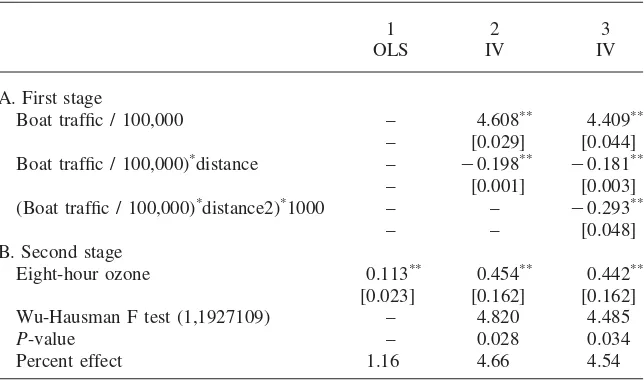
B. The Relationship between Boat Movements and Pollution
To assess the strength of our instrument, in Panel A of Table 3 we present evidence of the relationship between boat arrivals and departures on ozone levels in Los Angeles. It is highly statistically significant, witht-statistics that exceed 150 for both boat traffic in levels and boat traffic interacted with distance from port. Our estimates in the second column imply that each 500,000 tons of boat arrivals and departures (the approximate daily average) at the port increase ozone levels in the immediate area by 0.024 ppm, which is just over 60 percent of the mean ozone level in Long Beach of 0.039. This estimate is consistent with previous reports that suggest the port contributes to 50 percent of smog-forming gases (Polakovic 2002).
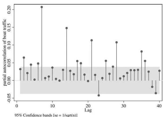
The interaction term between boat movement and distance from the port allows differential effects of port activity on resultant ozone levels depending on how far the area is from the port. We expect a greater impact on ozone levels in zip codes immediately adjacent to the port, with this effect diminishing as we travel away from the port. The negative interaction term, which is also highly statistically significant, is consistent with this. Figure 3 plots the effects of the average daily boat movement in the port on ozone levels based on the distance from the port. The results imply that the effect of the port on inland pollution levels is cut in half at 11 miles from the port and disappears at 23 miles from the port. We also add boat traffic interacted with a quadratic term in distance to allow a nonlinear decay from port emissions (Column 3 of Table 3). Although the quadratic term is statistically significant, Figure 3 shows that this addition does not appreciably change the spatial decay of pollution. These results highlight the strength of our first stage: arrivals and departures at the port have a significant effect on ozone levels in the immediately surrounding areas, and this effect diminishes as one moves away from the port. Boat arrivals and departures appear uncorrelated with other factors related to health, suggesting our
Table 3
OLS and IV regression results for effect of ozone on respiratory illnesses
1 2 3
OLS IV IV
A. First stage
Boat traffic / 100,000 – 4.608** 4.409**
– [0.029] [0.044]
Boat traffic / 100,000)*distance – ⳮ0.198** ⳮ0.181**
– [0.001] [0.003]
(Boat traffic / 100,000)*distance2)*1000 – – ⳮ0.293**
– – [0.048]
B. Second stage
Eight-hour ozone 0.113** 0.454** 0.442**
[0.023] [0.162] [0.162]
Wu-Hausman F test (1,1927109) – 4.820 4.485
P-value – 0.028 0.034
Percent effect 1.16 4.66 4.54
Notes: * significant at 5 percent, ** significant at 1 percent. N⳱1,927,187 in all regressions. Robust standard errors clustered by date in brackets. Dependent variable is the number of respiratory related hospital admissions per day, zip code, and age category. All regressions include controls for carbon mon-oxide, nitrogen dimon-oxide, maximum temperature, minimum temperature, precipitation, wind speed, humidity, cloud cover, age dummies, year-month dummies, day of week dummies, cubic day trend, and zip code fixed effects. “Percent effect” is the estimated percentage change in the dependent variables from 0.01 ppm increase in ozone based on the estimated ozone coefficient.
second-stage estimates will be consistent estimates of the biological effect of ozone on asthma hospitalizations.
C. The Relationship between Ozone and Hospitalizations
Turning to estimates of the relationship between ozone and health, we present OLS and IV results in Panel B of Table 3.32OLS results, shown in Column 1, indicate ozone has a statistically significant relationship with respiratory related hospitaliza-tions. A five-day increase in ozone of 0.01 ppm is associated with a modest 1.2 percent increase in hospitalizations. To gauge the sensibility of this estimate, we can compare it to estimates from previous epidemiological studies. A meta-analysis by Thurston and Ito (1999), which also focuses on all respiratory hospital admissions for all ages, finds a 1.5 percent increase in hospitalizations from a 0.01 ppm increase in ozone, an estimate quite comparable to ours.33
32. Our sample size of 1,927,187 comes from daily data from April-October from four age groups across roughly 350 zip codes in SCAQMD for eight years (1993-2000), less missing values.
-0.010 -0.005 0.000 0.005 0.010 0.015 0.020 0.025 0.030
0 2 4 6 8 10 12 14 16 18 20 22 24
Distance from port (miles)
O
zo
ne
(
ppm
)
linear -95% CI +95% CI quadatic
Figure 3
Effect of average daily port activity on ozone levels
Note: Results are based on regression coefficients from Columns 2 and 3 of Table 3.
When we turn to our IV estimates we find estimates that are nearly four times larger than OLS estimates. The considerably larger estimates, shown in Column 2, imply a 0.01 ppm increase in the five-day average ozone is associated with a 4.7 percent increase in hospitalizations. This difference is statistically significant ac-cording to a Hausman test, which has ap-value of 0.028. In Column 3, when we use the quadratic in distance, we find a similar 4.5 percent increase in hospitaliza-tions.
These estimates suggest that accounting for avoidance behavior, measurement error, and confounding increases estimates by a factor of four. Neidell (2009) finds estimates are roughly two times larger when controlling only for public air quality information. This difference is due to the fact that we also correct for measurement error, other unobserved sources of information for avoidance behavior, and potential confounding from other environmental factors, such as weather, suggesting the im-portance of accounting for these additional sources of bias.
Table 4
Sensitivity of regression results for effect of ozone on respiratory illnesses to weather and copollutants
1 2 3 4 5
A. OLS
Eight-hour ozone 0.113** 0.130** 0.118** 0.097** 0.105**
[0.023] [0.020] [0.023] [0.022] [0.027] B. IV—First stage
Boat traffic / 100,000 4.608** 4.733** 4.959** 4.037** 24.463**
[0.029] [0.035] [0.030] [0.031] [0.351] (Boat traffic /100,000)*distance ⳮ0.198** ⳮ0.192** ⳮ0.207** ⳮ0.187** ⳮ0.571**
[0.001] [0.001] [0.001] [0.001] [0.003] C. IV—Second stage
Eight-hour ozone 0.454** 0.465** 0.435** 0.451** 0.543**
[0.162] [0.168] [0.155] [0.171] [0.210]
Controls for weather Y N Y N Y
Controls for copollutants Y N N Y Y
Interactions with ozone N N N N Y
Notes: * significant at 5 percent, ** significant at 1 percent. N⳱1,927,187 in all regressions. Robust standard errors clustered by date in brackets. Dependent variable is the number of respiratory related hospital admissions per day, zip code, and age category. All regressions include age dummies, year-month dummies, day of week dummies, cubic day trend, and zip code fixed effects. “Weather controls” include maximum temperature, minimum temperature, precipitation, wind speed, humidity, and cloud cover. “Co-pollutant controls” includes carbon monoxide and nitrogen dioxide. For Column 5, ozone is interacted with weather and copollutant variables, and the coefficient shows the marginal effect of ozone evaluated at the mean of the weather and copollutant variables. All interactions are instrumented by boat arrivals and departures interacted with weather and copollutant variables, but only coefficients for boat arrivals and departures and distance from first stage are shown.
each weather variable and copollutant.34Our estimates are clearly insensitive to these alternative specifications, suggesting the strength of our instrument in controlling for potential confounding from environmental factors.
These cargo boats primarily emit NOx, but also emit particulate matter (PM), which raises an issue of whether our instrument meets the necessary exclusion re-strictions since PM affects health (Chay and Greenstone 2003a; Chay and Green-stone 2003b). Two correlation patterns across pollutants suggest this is not likely to be a major issue. One, the correlation between ozone and PM is very low. Ozone typically peaks in the summer because it forms in the presence of heat, whereas the other “criteria” pollutants, including PM, typically peak in the winter. For example, focusing on the Los Angeles region, Moolgavkar (2000) found a correlation with ozone of 0.20 for PM10 and 0.04 for PM2.5. Furthermore, our analysis focuses on the “ozone season”—the months of April-October—where many of these other
Table 5
Regression results for effect of ozone by type of respiratory illness
1 2 3 4
Any Respiratory
Illness
Pneumonia Bronchitis/
Asthma
Other Respiratory
Illnesses
A. OLS
Eight-hour ozone 0.113** 0.032* 0.038** 0.043**
[0.023] [0.014] [0.014] [0.011]
Percent effect 1.16 0.86 1.15 1.59
B. IV
Eight-hour ozone 0.454** 0.277** 0.145 0.032
[0.162] [0.101] [0.103] [0.080]
Percent effect 4.66 7.41 4.39 1.19
See notes to Table 3. Dependent variable is the number of hospital admissions per day, zip code, and age category, by type of respiratory illness.
lutants are at considerably lower levels they are unlikely to pose a health threat. Two, although we cannot directly control for PM,35it is highly correlated with both CO and NO2(Currie and Neidell 2005) so that including the two is likely to serve as a sufficient statistic for PM. Because our results are insensitive to excluding CO and NO2, we do not suspect the omission of PM to present a problem.
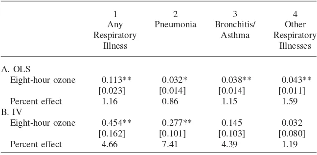
Becausee we have aggregated all respiratory illnesses and ozone may have a differential effect across the type of illnesses, in Table 5 we separately explore the effects of ozone on pneumonia (ICD 480-486), bronchitis and asthma (ICD 466, 490, 491, 493, 494), and other respiratory illnesses. Pneumonia, bronchitis, and asthma are conditions more likely to be exacerbated from current exposure, as op-posed to respiratory conditions like emphysema, where the effects from exposure are cumulative over time (Environmental Protection Agency 2006). Therefore, we expect larger effects for pneumonia and bronchitis and asthma than for other res-piratory conditions. The OLS results indicate fairly comparable effects across the conditions with a slightly larger effect, if anything, for other respiratory conditions. The IV results, however, paint a different picture. Consistent with expectations, the effects are largest for pneumonia, followed by bronchitis and asthma, and then a small effect for other respiratory illnesses.
We also perform a falsification test by specifying the dependent variable as ex-ternal injuries (fractures, dislocations, and sprains), an outcome that should not be affected by pollution levels. In our IV model, we find a statistically insignificant estimate of -0.161 with a standard error of 0.109. However, we also find a
cally insignificant effect of -0.008 when we estimate this by OLS. Therefore, while this test is useful in that it supports our preferred model, it is not definitive because it does not rule out a model we believe to be incorrect.
VII. The Cost of Pollution and Avoidance Behavior
Since there are no market prices for air quality, estimates of willing-ness to pay (WTP) are a key input for designing efficient environmental policy. We use our estimates to quantify the WTP to reduce ozone levels in the Los Angeles area. Based on our expressions for WTP in section IV (WTP⳱ ␦h/␦ozone*(mⳭ w)), for ␦h/␦ozone we use our estimates from Table 3, form we use the average hospital bill for any respiratory related admissions ($22,438) and forw we use the average length of stay for this admission (6.5 days) multiplied by the average hourly wage of $16/hour in the Los Angeles area. We recognize that this measure likely understates the full value because it ignores any direct effects on well-being not included in hospital costs and it ignores other health episodes that do not result in hospitalizations.36
Given that the mean eight-hour ozone exposure is 0.05 ppm in the months from April to October (Table 1) and 0.025 ppm in the months from October to April, our OLS estimates, which likely reflects cost of illness (COI) estimates, indicate that ozone costs $11.1 million per year in the Los Angeles region.37Based on the IV estimates, which more closely resemble WTP estimates, the cost amounts to $44.5 million per year. Comparable estimates for a 0.01 ppm change in ozone are $2.8 million using OLS and $11.2 million using IV.38These differences gives a sense of how a more simplified analysis based on OLS, and thus COI, would vastly under-estimate the full costs of ozone exposure.
We also can use these two estimates along with estimates from Neidell (2009) to present bounds on the cost of avoidance behavior. Since our IV estimates differ from OLS by more than just whether they account for avoidance behavior—they also correct for measurement error and environmental confounding—the simple differ-ence between the WTP and COI estimates of $33.4 million gives an upper bound on the cost of avoidance behavior. Using the estimates from Neidell (2009) that suggest production function estimates two times larger than dose response estimates yields an estimate of WTP of $22.1 million. Since this estimate is likely to understate WTP, the $11.1 million difference from COI gives a lower bound on the cost of avoidance behavior. Although our estimated range of $11.1 to $33.4 million for avoidance behavior is wide, it is a large fraction of total costs, thus demonstrating
36. Estimates are comparable if we aggregate the separate impacts for the different respiratory illness explored in Table 5.
37. Consistent with our econometric models, we assume a linear effect of ozone on health. To obtain this estimate, we multiply our coefficients by the number of Age Groups 4, the number of ZIP codes in SCAQMD (339), and the number of days in the two seasons (214 and 151, respectively), and divide by the number of days we average ozone levels more than five.
the importance of accounting for avoidance behavior in understanding the societal costs of pollution.
VIII. Conclusion
A pervasive problem in the literature on the costs of pollution is that optimizing individuals may compensate for increases in pollution by reducing their exposure to protect their health. Furthermore, using ambient monitors to approximate individual exposure to pollution may induce considerable measurement error. More-over, fully accounting for all environmental factors that correlate with both pollution and health, such as weather and allergens, presents a major obstacle. Estimates of the costs of pollution that do not properly address these issues may be significantly biased.
We propose a novel approach to estimate the effects of ozone on health and its associated costs on society. We isolate the short-term effect of ozone holding com-pensatory behavior fixed, limiting environmental confounding, and accounting for measurement error by using boat arrivals and departures at the Ports of Los Angeles and Long Beach as an instrument for ozone levels. Since boat traffic is unobserved by most residents, it generates an important source of variation in pollution that is difficult to avoid and cannot easily be offset by residents’ compensatory behavior.
We find that OLS estimates of ozone on hospitalization are small. In contrast, instrumental variable estimates indicate a considerably larger effect of ozone con-centrations on respiratory related hospitalizations. Based on our models, we calculate that the cost of ozone in Los Angeles is at least $44 million per year. Furthermore, the cost of avoidance behavior ranges from $11.1 to $33.4 million per year depend-ing on assumptions about measurement error and environmental confounddepend-ing. While these estimates cover a wide range, they are at least as large as the medical and wage expenditures based on a cost of illness analysis, suggesting considerable costs from this nonmarket behavior.
References
Alberini, Anna, and Alan Krupnick. 2000. “Cost-of-Illness and Willingness-to-Pay Estimates of the Benefits of Improved Air Quality: Evidence from Taiwan.”Land Economics 76(1):37–53.
AQMD. 2002. “AQMD Makes Progress in Cleaning up Air Pollution at Ports.”AQMD News, August 20.
Bell, Michelle, Aidan McDermott, Scott Zeger, Jonathan Samet, and Francesca Dominici. 2004. “Ozone and Short-Term Mortality in 95 U.S. Urban Communities, 1987-2000.” Journal of the American Medical Association292(19):2372–78.
Chang, L., Petros Koutrakis, Paul Catalano, and Helen Suh. 2000. “Hourly Personal Exposures to Fine Particles and Gaseous Pollutants.”Journal of the Air and Waste Management Association50(7):1223–35.
Chay, Kenneth, and Michael Greenstone. 2003a. “Air Quality, Infant Mortality, and the Clean Air Act of 1970.” NBER Working Paper 10053.
———. 2003b. “The Impact of Air Pollution on Infant Mortality: Evidence from Geographic Variation in Pollution Shocks Induced by a Recession.”Quarterly Journal of Economics118(3):1121–67.
Cropper, Maureen, and A. Myrick Freeman, III. 1991. “Valuing Environmental Health Effects.” InMeasuring the Demand for Environmental Commodities, ed. John Braden and Charles Kolstad Amsterdam: North-Holland.
Currie, Janet, and Matthew Neidell. 2005. “Air Pollution and Infant Health: What Can We Learn from California’s Recent Experience?”Quarterly Journal of Economics
120(3):1003–30.
———. 2007. “Climate Change, Mortality and Adaptation: Evidence from Annual Fluctuations in Weather in the U.S.” NBER Working Paper 13178.
Deschenes, Olivier, and Enrico Moretti. 2009. “Extreme Weather Events, Mortality and Migration.”Review of Economics and Statistics91(4):659–81.
Environmental Protection Agency. 1999. “Guidelines for Reporting of Daily Air Quality— Air Quality Index (AQI).” EPA Document #454-R-99-010, Research Triangle Park, NC. ———. 2000. “Analysis of Commercial Marine Vessels Emissions and Fuel Consumption
Data.” EPA Report Number 420-R-00-02.
———. 2006.Air Quality Criteria Document for Ozone. Washington, D.C.: Environmental Protection Agency.
Dominici, Francesca, Jonathan Samet, and Scott Zeger. 2000. “Combining Evidence on Air Pollution and Daily Mortality from the 20 Largest U.S. Cities: A Hierarchical Modeling Strategy.”Journal of the Royal Statistical Society163(3):263–302.
Friedman, Michael, Kenneth Powell, Lori Hutwagner, LeRoy Graham, and W. Gerald Teague. 2001. “Impact of Changes in Transportation and Commuting Behaviors During the 1996 Summer Olympic Games in Atlanta on Air Quality and Childhood Asthma.” Journal of the American Medical Association285(7):897–905.
Gajendran, Prakash, and Nigel Clark. 2003. “Effect of Truck Operating Weight on Heavy-Duty Diesel Emissions.”Environmental Science and Technology37(18):4309–17. Harrington, Winston, and Paul Portney. 1987. “Valuing the Benefits of Health and Safety
Regulation.”Journal of Urban Economics22(1):101–12.
Jerrett, Michael, Richard Burnett, C. Arden Pope, III, Kazuhiko Ito, George Thurston, Daniel Krewski, Yuanli Shi, Eugenia Calle, and Michael Thun. 2009. “Long-Term Ozone Exposure and Mortality.”New England Journal of Medicine360(11):1085–95.
Knittel, Christopher R., Douglas Miller, and Nicholas J. Sanders. 2009. “Caution, Drivers! Children Present. Traffic, Pollution, and Infant Health.”University of California-Davis. Unpublished.
Lin, Tsai-Yin, Li-Hao Yuong, and Chiu-Sen Wang. 2001. “Spatial Variations of Ground Level Ozone Concentrations in Areas of Different Scales.”Atmospheric Environment 35(33): 5799–807.
Lleras-Muney, Adriana. 2009. “The Needs of the Army: Using Compulsory Relocation in the Military to Estimate the Effect of Environmental Pollutants on Children’s Health.” Journal of Human Resources. Forthcoming.
Moolgavkar, SH. 2000. “Air Pollution and Daily Mortality in Three U.S. Counties.” Environmental Health Perspectives108(8):777–84.
Neidell, Matthew. 2004. “Air Pollution, Health, and SocioEconomic Status: The Effect of Outdoor Air Quality on Childhood Asthma.”Journal of Health Economics23(6):1209– 36.
———. 2009. “Information, Avoidance Behavior, and Health: The Effect of Ozone on Asthma Hospitalizations,”Journal of Human Resources44(2):450–78.
Polakovic, Gary. 2002. “Finally Tackling L.A.’s Worst Air Polluter.”The Los Angeles Times, February 10.
Racherla, P. N., and P. J. Adams. 2009. “US Ozone Air Quality under Changing Climate and Anthropogenic Emissions.”Environ Sci Technol43(3):571–77.
Thurston, G.D., and K. Ito. 1999. “Epidemiological Studies of Ozone Exposure Effect.” In Air Pollution and Health, ed. S.T. Holgate, J.M. Samet, H.S. Koren, and R.L. Maynard. San Diego, Calif.: Academic Press.
Cathryn, Tonne, Robin Whyatt, David Camann, Frederica Perera, and Patrick Kinney. 2004. “Predictors of Personal Polycyclic Aromatic Hydrocarbon Exposures among Pregnant Minority Women in New York City.”Environmental Health Perspectives112(6):754–59. Wald, Matthew. 2007. “Southern California Ports Move to Curb Emissions from Shipping