Fitness distributions in evolutionary computation:
motivation and examples in the continuous domain
Kumar Chellapilla
a, David B. Fogel
b,*
aDepartment of Elect.Comp.Engg.,UCSD,La Jolla,CA92037,USA bNatural Selection,Inc.,3333N.Torrey Pines Ct.,Ste.200,La Jolla,CA92037,USA
Received 25 January 1999; accepted 11 June 1999
Abstract
Evolutionary algorithms are, fundamentally, stochastic search procedures. Each next population is a probabilistic function of the current population. Various controls are available to adjust the probability mass function that is used to sample the space of candidate solutions at each generation. For example, the step size of a single-parent variation operator can be adjusted with a corresponding effect on the probability of finding improved solutions and the expected improvement that will be obtained. Examining these statistics as a function of the step size leads to a ‘fitness distribution’, a function that trades off the expected improvement at each iteration for the probability of that improvement. This paper analyzes the effects of adjusting the step size of Gaussian and Cauchy mutations, as well as a mutation that is a convolution of these two distributions. The results indicate that fitness distributions can be effective in identifying suitable parameter settings for these operators. Some comments on the utility of extending this protocol toward the general diagnosis of evolutionary algorithms is also offered. © 1999 Elsevier Science Ireland Ltd. All rights reserved.
Keywords:Fitness distributions; Evolutionary computation; Continuous domain
www.elsevier.com/locate/biosystems
1. Introduction
When used for function optimization, evolu-tionary computation relies on a population of contending solutions to a problem at hand, where each individual is subject to random variation
(mutation, recombination, etc.) and placed in competition with other extant solutions. Random variation provides a means for discovering nov-elty while selection serves to eliminate those trials that do not appear worthwhile in the context of the given criterion. Thus evolutionary algorithms can be seen as performing a search over a state space S of possible solutions.
In essence, most evolutionary algorithms can be described by the difference equation
x[t + 1] = s(6(x[t])) (1)
* Corresponding author. Tel.: +1-619-4556449; fax: + 1-619-4551560.
E-mail addresses: [email protected] (K. Chellapilla), [email protected] (D.B. Fogel)
where x[t] is the population at time t under representation x, 6 is the variation operator(s), and s is the selection operator. The stochastic elements of this difference equation include6, and often s, and the initialization mechanism for choosingx[0]. The choices made in terms of rep-resentation, variation, selection, and initialization shape the probability mass function that describes the likelihood of choosing solutions fromSat the next iteration. Alternative choices can lead to dramatically different rates and probabilities of improvement at each iteration.
The question of how to design evolutionary search algorithms to improve their optimization performance has been given significant consider-ation, but few practical answers have been iden-tified. Indeed, many supposed answers have in fact been false leads, dogmatically repeated over many years such that they have almost become ‘conventional wisdom’. Only recently have several of these generally accepted central tenets of evolu-tionary algorithms been questioned and exposed as being misleading or simply incorrect. Four of these erroneous tenets are detailed here.
1.1. Binary representations and maximizing implicit parallelism
Holland (1975) pp. 70 – 71, speculated that bi-nary representations would provide an advantage to an evolutionary algorithm. The rationale un-derlying this claim relied on the notion of maxi-mizing implicit parallelism in schemata. To review the concept, a schema is a template from some alphabet of symbols, A, and a wild card symbol
c that matches any symbol in A. For example, given a binary alphabetA, the schema [10c c] is a template for the strings [1000], [1001], [1010], and [1011]. Holland (1975) pp. 64 – 74, offered that any evaluated string (encoding a possible solution to a task at hand) actually offers partial information about the expected fitness of all pos-sible schemata in which that string resides. That is, if string [0000] is evaluated to have some fitness, then partial information is also received about the worth of sampling from variations in
[c c c c], [0c c c], [c0c c], [c00c],
[c0c0], and so forth. This characteristic is
termed intrinsic parallelism (or implicit paral
-lelism), in that through a single sample, informa-tion is gained with respect to many schemata.
If information were actually gained by this process of implicit sampling, it would seem rea-sonable to expect that maximizing the number of schemata that are processed in parallel would be beneficial (Holland 1975). For any representation that is a bijective mapping from the state space of possible solutions to the encoded individuals, im-plicit parallelism is maximized for the smallest cardinality of alphabet. That is, given a choice between using a binary encoding or any other cardinality, binary encodings should be preferred. The emphasis on binary representations, specifi-cally within genetic algorithms (GAs), was so strong that Antonisse (1989) wrote ‘‘the bit string representation has been raised beyond a common feature to almost a necessary precondition for serious work in the GA’’.1
More careful inspection of this issue, however, indicates immediate problems with the claim that there should be an advantage to binary encodings. Of primary concern is the choice of binary encod-ing. Radcliffe (1992) noted that there are many binary representations of solutions in S. For ex-ample, if S={1, 2, 3, 4}, then there are 4! differ-ent binary represdiffer-entations of these solutions. One would be {1, 2, 3, 4}{00, 01, 10, 11}, while
another would be {1, 2, 3, 4}{11, 01, 00, 10}. It
is easy to show empirically that the performance of evolutionary algorithms which employ different binary representations for the same problem do not exhibit similar performance (see De Jong et al., 1995, described below), and for some binary representations, performance is worse that a com-pletely random search. This provides a counterex-ample to the claim of optimality of binary encodings (and moreover the ‘principle of mini-mum encoding’, proposed in Goldberg, 1989).
Fortunately, binary encodings are often clumsy, and many researchers abandoned the practice of
1The fundamental impact of binary representations on
using binary encodings in the late 1980s and early 1990s, finding more convenient representations for their problems, and also better results (An-tonisse, 1989; Koza, 1989; Davis, 1991, p. 63; Michalewicz, 1992; Ba¨ck and Schwefel, 1993; Fogel and Stayton, 1994). More recently, Fogel and Ghozeil (1997a) proved that it is possible to create completely equivalent evolutionary al-gorithms on any problem regardless of the cardi-nality of a bijective representation. Thus there is provably no information gained or lost as a con-sequence of simply altering the cardinality of rep-resentations (cf. Holland, 1975).
1.2. Crosso6er and building blocks
In addition to advocating the use of binary representations, Holland (1975) also strongly ad-vocated the use of one-point crossover as a mech-anism to combine ‘building blocks’ from different solutions, and simultaneously minimized the im-portance of random mutation. More recently, Holland (1992) offered that early efforts to simu-late evolution ‘‘fared poorly because they… relied on mutation rather than mating’’. The supposed importance of crossover and relative unimpor-tance of mutation has been echoed in Goldberg (1989), Davis (1991), Koza (1992), and many others. And yet, several problems with this ap-proach have been discovered.
With regard to processing building blocks (i.e. schemata that are associated with above-average performance), suppose that one particular build-ing block was [1c…c0], that is, determining the first and last positions in a string to be 1 and 0, respectively, defines the building block. When one-point crossover is applied, it will always dis-rupt this building block. A natural solution to this problem is to view individuals not as strings, but as rings, and use two-point crossover to cut and splice segments of solutions. Once two-point crossover is invented, it is an easy step to move to uniform crossover, where each component in an offspring is selected at random from either of two parents.
If evolution proceeds best when it combines building blocks, it would be easy to speculate that uniform crossover would not perform as well as
one- or two-point crossover because rather than preserve such blocks of code, it tends to disrupt them. Yet, the empirical evidence offered in Syswerda (1989) showed uniform crossover out-performing both one- and two-point crossover on several problems including the traveling salesman (TSP) and the onemax (counting ones) problems. Fogel and Angeline (1998) observed similar re-sults comparing these operators in solving linear systems of equations. Moreover, there have been many studies generating empirical evidence that evolutionary algorithms which do not rely on crossover can outperform or perform comparably with those that do (Reed et al., 1967; Fogel and Atmar, 1990; Ba¨ck and Schwefel, 1993; Angeline, 1997; Chellapilla, 1997, 1998a; Fuchs, 1998; Luke and Spector, 1998). Jones (1995) even demon-strated that crossing extant parents with com-pletely random solutions (dubbed ‘‘headless chicken crossover’’) could outperform structured recombination on several problems (see Fogel and Angeline (1998) for further supportive evidence).
De Jong et al. (1995) showed unequivocally that there is an important synergy between opera-tor and representation. They first considered the problem of assigning the four values {1, 2, 3, 4} to binary strings {00, 01, 10, 11}, respectively, under the fitness function:
f(y) = integer(y) + 1 (2)
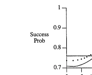
For a population ofn=5, De Jong et al. (1995) enumerated a Markov chain that completely de-scribes the probabilistic behavior of an evolution-ary algorithm on this problem. Fig. 1 shows the probability of having the evolving population contain the best possible solution as a function of the number of generations both when using or not using crossover. The performance of random
search is provided for comparison. Here,
ver-sion of evolutionary algorithm for at least the first ten generations. In the first equivalence class, applying crossover to the second- and third-best solutions can generate the global optimum. In the other two classes, it cannot. Thus the chosen
Fig. 3. The exact probability of the population containing the best solution to the problem shown in Fig. 2 for the third equivalence class of representations (from De Jong et al., 1995). Here, no crossover outperforms the use of crossover by a wider margin across all generations consistently. Note too that random search alone outperforms both crossover and the absence of crossover for about the first ten generations. The results indicate the importance of matching the variation operator with the representation.
Fig. 1. The exact probability of containing the best solution as a function of the number of generations when using a simple genetic algorithm to optimizef(y)=integer(y)+1 under rep-resentation {00, 01, 10, 11} mapped to {1, 2, 3, 4} (from De Jong et al., 1995). Here crossover is seen to outperform the absence of crossover regardless of the number of generations. However, this mapping is only one of 4! different possible mutations. Of these possibilities, three equivalent classes emerge. The other two classes of behavior are shown in Figs. 2 and 3.
representation cannot be considered in isolation from the search operator.
This has been more broadly proved in the ‘no free lunch’ theorems of Wolpert and Macready (1997). For algorithms that do not resample points in S, across all possible problems, all al-gorithms perform the same on average.2
When an algorithm is tailored to a particular problem, it will of necessity perform worse than random search on some other problem. Thus there cannot be one best variation operator across all prob-lems. Crossover, in all its forms, can be seen in this context simply as one possible choice that the human operator can make. Its effectiveness is problem and representation dependent.
1.3. The schema theorem:the fundamental theorem of genetic algorithms
Holland (1975) offered a theorem that describes the average propagation of schemata from one generation to the next under the influence of
Fig. 2. The exact probability of the population containing the best solution to the problem shown in Fig. 1 for the second equivalence class of representations (from De Jong et al., 1995). Here, no crossover outperforms the use of crossover by a small margin across all generations consistently.
2Salomon (1996) studied the relevance of resampling in
proportional selection and variation operators such as one-point crossover and mutation. Omit-ting the effects of variation operators, the formula is:
EP(H,t+1)=P(H,t)f(H,t)
f( (3)
where H is a particular schema (hyperplane),
f(H,t) is the mean fitness of solutions that contain
Hat timet,f( is the mean fitness of all solutions in the population, and P(H,t) is the proportion of solutions that contain H at time t. Thus the expected frequency of H in the next time step is proportional to its current frequency and its rela-tive fitness. Extrapolating, Goldberg (1989), p. 33, concluded that above-average schemata receive exponentially increasing trials in subsequent gen-erations and offered this result as being of such importance that it is named the ‘Fundamental Theorem of Genetic Algorithms’.
Radcliffe (1992) noted that the theorem applies to all schemata in a population, even when the schemata defined by a representation may not capture the properties that determine fitness. For example, if the objective is to maximize the in-teger value of a binary string, then the strings [1000] and [0111] are as close as possible in terms of fitness (8 vs. 7), and yet they share no sche-mata. Thus the intuition that proportional selec-tion will tend to emphasize those schemata that share important features related to fitness may not hold in practice.
Most work in genetic algorithms no longer uses proportional selection, so the ‘fundamental’ im-portance of the schema theorem can immediately be questioned. Moreover, the conclusion that above-average schemata will continue to receive exponentially increasing attention omits the con-sideration that the theorem only describes the
expected behavior in asingle generation. There is no reason to believe that the equation can be extrapolated over successive generations without giving explicit consideration to the variance of the process as well as its expectation. But more sig-nificantly, Fogel and Ghozeil (1997b) proved that the schema theorem does not apply when the fitness of schemata are described by random vari-ables, as is often the case in real-world
applica-tions. The theorem only applies to the specific population in question and the specific fitness values assigned to each individual in that population.
Even more importantly, the theorem cannot address the issue of how new solutions are discov-ered; it can only indicate the statistical expecta-tion of reproducing already existing soluexpecta-tions in proportion to their relative fitness. It cannot esti-mate long-term proportions of schemata with reli-ability because this depends strongly on the likelihood of new solutions being generated by variation.
1.4. Proportional selection and the k-armed bandit
Holland (1975) made an analogy between the problem of how best to sample from competing schemata within a population and how best to sample from ak-armed bandit (i.e. a slot machine with k arms). The payoff from each arm of the bandit has a mean and variance, and the analysis centered on how best to sample the arms so as to minimize expected losses over those samples. The conclusion was essentially to sample in proportion to the observed payoff from each arm, which led to the use of proportional selection in genetic algorithms, and the resulting focus on the schema theorem.
Unfortunately, insufficient attention was given to this analysis in two regards. The first is the choice of criterion: Minimizing expected losses does not correspond with the typical problem of function optimization that demands discovering the single best solution. In order to minimize expected losses between two choices, the proper sampling is to devote all trials to the choice with the greater average payoff. But this choice may prohibit discovering the best possible solution. Consider the case where there are four possible solutions to a problem with corresponding fitness values as shown:
[00]=19, [01]=0, [10]=11, [11]=9
expected losses, trials should be allocated to [1c], but this would then preclude discovering the best solution [00].
The second respect is more fundamental: The claim that the analysis in Holland (1975) leads to an optimal sampling plan has been shown to be mathematically flawed both by counterexample (Rudolph, 1997) and direct analysis (Macready and Wolpert 1998). Proportional selection does not minimize expected losses, so even if this crite-rion is given preference, the development in
Hol-land (1975) does not support the use of
proportional selection in evolutionary algorithms. This form of selection is just one among many options, and the choice should be based on the dependencies posed by the particular problem.
1.5. A new direction
Certainly, the above list could be extended (e.g. inversion was offered to reorder schemata for effective processing as building blocks by one-point crossover (Holland, 1975; pp. 106 – 109), but this has had no general empirical support (Davis, 1991; Mitchell, 1996; Lobo et al., 1998). In light of these missteps, it would appear appropriate to investigate new methods for assessing the funda-mental nature of evolutionary search and opti-mization. The formulation in Eq. (1) leads directly to a Markov chain view of evolutionary al-gorithms in which a time-invariant, memoryless probability transition matrix describes the likeli-hood of transitioning to each possible population configuration given each possible configuration (Fogel, 1994; Rudolph, 1994 and others). Such a description immediately leads to answers regard-ing questions about the asymptotic behavior of various algorithms (e.g. typical instances of evolu-tion strategies and evoluevolu-tionary programming ex-hibit asymptotic global convergence (Fogel, 1995a), whereas the canonical genetic algorithm (Holland, 1975) is not convergent due to its re-liance on proportional selection (Rudolph, 1994)). Further, as shown above, De Jong et al. (1995) used Markov chains and brute force computation to analyze the exact transient behavior of genetic algorithms under small populations (e.g. size five) and small chromosomes (e.g. two or three bits)
concentrating on the expected waiting time until the global optimum is found for the first time. But this procedure appears at present to be too com-putationally intensive to be useful in designing more effective (in terms of quality of evolved solution) and efficient (in terms of rate of conver-gence) evolutionary algorithms for real problems. The description offered by Eq. (1), however, suggests that some level of understanding of the behavior of an evolutionary algorithm can be garnered by examining the stochastic effects of the operators sand6on a populationx at timet. Of interest is the probabilistic description of the fitness of the solutions contained in x[t+1]. Re-cent efforts (Altenberg, 1995; Fogel, 1995a; Grefenstette, 1995; Fogel and Ghozeil, 1996) have been directed at generalized expressions describing the relationship between offspring and parent fitness under particular variation operators, or empirical determination of the fitness of offspring for a given random variation technique. This pa-per offers evidence that this approach to describ-ing the behavior of an evolutionary algorithm can be used to design more efficient and effective optimization techniques.
2. Background on methods to relate parent and offspring fitness
Altenberg (1995) offered the conjecture that, rather than rely on the schema theorem, the per-formance of an evolutionary algorithm could be better estimated by examining the probability mass function:
Pr(W = w(x); w(y), w(z)) (4)
Grefenstette (1995) offered a similar notion for assessing the suitability of various genetic opera-tors. Attention was focused on the mean fitness of the offspring generated by applying a genetic op-erator to a parent conditioned on the parents’ fitness. That is, the fitness distribution of an oper-ator was defined as:
FDop(Fp) = Pr(FcFp) (5)
where the fitness distribution of an operatorFDop
is the family of probability distributions of the fitness of the offspring Fc, indexed by the mean
fitness of the parents Fp. It was shown that the
mean of the fitness distribution for some genetic operators could be described by simple linear functions of Fp.
This analysis, although potentially insightful, suffered from two important drawbacks. First, attention was unfortunately limited to the case of proportional selection and second, and more im-portantly, the analysis turns on relevance of the correlation in fitness between parent and off-spring. For example, Grefenstette (1995) offered that if the fitness distribution of an operator were shown to be independent of the parent’s fitness then poor performance (‘failure’) should be ex-pected. But this can be contradicted by counterex-ample. For a Newton – Gauss search on a quadratic bowl, regardless of the position of the parent, and therefore its fitness, the offspring generated will be at the global optimum and have minimum error. Thus offspring fitness is indepen-dent of parental fitness, yet the algorithm is as successful as possible on this function.
The emphasis on correlation between parental fitness and offspring fitness goes back at least to Manderick et al. (1991). The utility of this ap-proach can suffer when attention is focused on the correlation between mean parental fitness and mean offspring fitness. For example, for the case of linear fitness functions, under real-valued rep-resentations the use of zero mean Gaussian muta-tions yields zero mean difference between parent and offspring fitness regardless of the setting for the step size control parameter s (the standard deviation). But the expected rate of convergence for these methods depends crucially on the setting of s, as summarized in Ba¨ck (1996) and Fogel (1995a).
In contrast, rather than examine mean parental fitness and how it correlates to mean offspring fitness for a particular search operator, attention can be more fruitfully given to the expected rate of improvement (in terms of mean progress to-ward the optimum), as was offered in Rechenberg (1973). For the case of searching in Rnusing zero
mean Gaussian mutations, Rechenberg (1973) noted that the maximum expected rate of conver-gence was attained for two simple functions, the sphere and corridor models, when the probability of a successful mutation was approximately 0.2. Thus, the 1/5 rule was suggested:
The ratio of successful mutations to all muta-tions should be 1/5. If this ratio is greater than 1/5, increase the variance; if it is less, decrease the variance.
Schwefel (1981) suggested measuring the suc-cess probability on-line over 10n trials (where there are n dimensions) and adjusting s at itera-tion t by:
cesses in 10n trials divided by 10n. This allowed for a general solution to setting the step size, but the robustness of this procedure remains un-known in general.
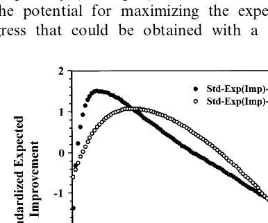
Fogel (1995b) and Fogel and Ghozeil (1996) empirically examined the distribution of fitness scores attained under different variation operators for specific parameter settings on three continuous optimization problems (sphere, Rosenbrock, Bo-hachevsky) and one discrete problem (travelling salesman problem (TSP)). For the continuous problems, the variation operators included zero mean Gaussian mutations and different forms of recombination (one-point, intermediate). In con-trast, a variable-length reversal of a segment of the list of cities to be visited was tested for the TSP. Experiments involved repeated Monte Carlo application of variation operators to parents from an initial generation, with the probability of im-provement and expected amount of imim-provement (i.e. the reduction in error) being recorded for each trial. The mean behavior of the operators as a function of their parametrization was depicted graphically (see Fig. 4), and consistently showed the potential for maximizing the expected pro-gress that could be obtained with a particular
operator by adjusting its control parameter and its associated probability of improvement. The results demonstrated the possibility for optimizing variation operators even when no analytic deriva-tion for optimal parameters settings may be possible.
Following Fogel and Ghozeil (1996), the method is further developed here and used to examine the appropriate settings for scaling three different types of single-parent variation operators across a set of four continuous function optimiza-tion problems in 2, 5, and 10 dimensions. The results indicate that the expected improvement of an operator can be estimated for various control parameters; however, in contrast to the 1/5 rule it may be insufficient to use the probability of im-provement as a surrogate variable to maximize the expected improvement.
3. Methods
To begin, three sets of experiments were per-formed to investigate the properties of three
varia-tion operations that are common in the
application of evolutionary algorithms to continu-ous function optimization problems. The frame-work for selection is based on the (1, 100) model, indicating that a single parent generates 100 off-spring, and then the best of these offspring is selected to be the parent for the next generation. Attention was given to the probability of im-provement (PI) and the expected improvement (EI) attained by the application of a particular variation operator. The algorithm proceeded as follows:
(i) The trial number, t, was set to 1.
(ii) 100 initial solutions (parents) xi(t), i=1,…,
100 were sampled uniformly from an interval [a,b]n
.
(iii) Each parent was evaluated in light of the objective function F(x) (defined below).
(iv) The best parentx(t) with the lowest objec-tive value was used to generate 100 offspring,
x%i(t), i=1,…, 100 through 100 independent ap-plications of a variation operator6. The variation 6 was accomplished in the form:
Fig. 5. The probability density function (pdf) of the standard Gaussian and Cauchy pdfs in comparison with their convolu-tion. The convolution of the pdfs is equivalent to taking the mean of the random variables. There exists a trade-off among the three pdfs between the probabilities of generating very small (0.0 – 0.6); small (0.6 – 1.2); medium (1.2 – 2.0); large (2.0 – 4.8); and very large (\4.8) mutations. These were the pdfs
used for generating 100 offspring from the best parentsx(t) (Eq. (6)).
Steps (i) – (vii) were repeated for 5000 trials in a Monte Carlo fashion whereupon the mean f(t) and I(t) were recorded as estimates of PIandEI
for the variation operator 6 with scaling term s. For convenience, PI and EI are used to denote these estimates in the following discourse. The values of sare identified later in this section.
Each experiment was conducted on four test functions, F1–F4, given by:
Function F1 is the sphere, F2 is a modified
version of the Ackley function, F3is the Rastrigin
function, and F4 is the generalized step function.
The three different variation operators were performed as:
x%i,j=x*j+sNj(0,1) (12)
x%i,j=x*j+sCj(0,1) (13)
x%i,j=x*j+0.5s(Nj(0,1)+Cj(0,1)) (14)
where N(0,1) is a standard normal RV, C(0,1) is a standard Cauchy RV, j is an index for the jth dimension, and i is an index for theith offspring from x. For the case of Gaussian mutation, sis the standard deviation s, but recall that the
stan-dard deviation of a Cauchy pdf is undefined, thus
s is best viewed simply as a scaling factor. Throughout the remainder of the paper, these three variations are described as Gaussian, Cauchy, and mean mutation operators (GMO, CMO, and MMO, respectively).
For each function F1–F4, 200 separate
experi-ments (each of 5000 trials) were conducted by stepping the value of s from 0.01 to 4.00 by increments of 0.02. Initial solutions were
dis-x%i(t) = x(t) + 6 (6)
where6was a random variable with one of three possible probability density functions (pdfs): (1) a zero mean Gaussian random variable with stan-dard deviation (scaling parameter) s; (2) a stan-dard Cauchy random variable scaled by s; (3) a convolution of (1) and (2). These variation opera-tors follow typical implementations in evolution-ary computation for real parameter optimization (Ba¨ck, 1996; Rudolph, 1997; Chellapilla, 1998b). Fig. 5 indicates the pdf for each choice.
(v) Each offspring was evaluated in light of
F(x).
(vi) The fraction of offspring, f(t), that were strictly better (i.e. lower error) than x(t) was computed.
(vii) The offspring with lowest error,x%(t), was used to compute the improvement during trial t
using
I(t) = F(x(t))−F(x%(t)) (7)
Note thatI(t) could be negative if the best of the 100 offspring was worse than the parent that generated it.
tributed uniformly over [−4,4]n, (
n=2, 5, and 10) which is symmetric about the optimum solu-tion.
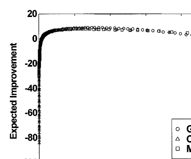
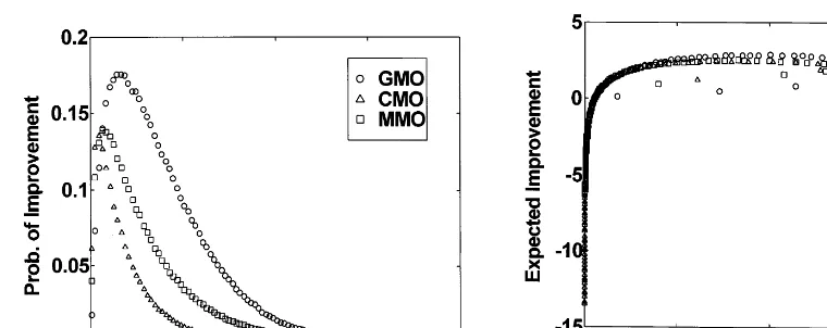
Fig. 8. The PIfor the GMO, CMO, and MMO across the settings of the step size, s, for the 10-dimensional sphere function (F1). For all three operators, thePIvalues decrease
with increasing sigma. Since the quadratic function is continu-ous and unimodal, thePIvalue attains a peak value of 0.5 as stends to 0, which is thePIvalue on an inclined plane. ThePI curve for the CMO drops the fastest and is followed by those for the MMO and GMO. Paralleling the estimates forEI(Fig. 7), the GMO offers the greatest PIfor any fixed value ofs, followed by MMO and CMO, respectively. For s0 the
PI0.5, and assbecomes large thePItends to zero.
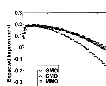
Fig. 6. The EIfor the GMO, CMO, and MMO across the settings of the step size,s, for the 2-dimensional sphere func-tion (F1). The CMOEIcurve peaks first, followed by those for
the GMO and MMO. The maximum EIoccurs at s=0.47, 0.49, and 0.21 for the GMO, MMO, and CMO, respectively. The corresponding peakEIvalues were 0.20, 0.19, and 0.20 for the GMO, MMO, and CMO, respectively. The GMO curve has the largest bandwidth, followed by those for the MMO and CMO.
4. Results
Figs. 6 and 7 show the meanEIas a function of
s for the GMO, CMO, and MMO on the 2- and 10-dimensional sphere (F1). Certain similar
pat-terns are evidenced immediately. First, in both cases, the GMO offers a greater peak EI than does the MMO or CMO. In addition, the peakEI
occurs for GMO, MMO, and CMO with decreas-ing values of s. That is, larger s values are re-quired to generate the peakEIfor GMO than are required for either MMO or CMO. As expected, fors0 theEI0, and assbecomes large theEI
turns negative (i.e. the typical step size of the variation operator is larger than twice the distance to the optimum and the resulting offspring are worse than their parent). Fig. 8 shows the PIfor each operator on the 10-dimensional F1.
Parallel-ing the estimates for EI, the GMO offers the greatest PI for any fixed value of s, followed by MMO and CMO, respectively. Fors0 thePI
0.5, and as sbecomes large the PItends to zero. Of particular interest is the corresponding rela-tionship between PIand EIfor each operator on
Fig. 9. The relationship between thePIandEIfor the GMO, CMO, and MMO on the 10-dimensional sphere function (F1).
For very smallPIthere is a corresponding negativeEI regard-less of the variation operator, but asPIincreases there is a wide range of values that correspond to essentially similar values ofEI.
there is a wide range of values that correspond to essentially similar values ofEI. Table 1 shows the
PI associated with the peak EIfor each operator for the 10-dimensional F1 (and other functions).
As indicated, regardless of the variation operator the best choice for PIis considerably less than 0.2 (cf. the 1/5 rule).
One method for assessing the robustness of a particular variation operator concerns the range of values forsthat will yield reasonable values of
EI. For the case of unimodal fitness distribution curves, define the bandwidth to be the range of values ssuch that
EI(s) \ 0.5 EI* (21)
where EI(s) is the expected improvement for a scaling value s and EI* is the peak EI. Table 2 indicates that the bandwidth for the GMO was almost twice as wide as for the CMO. In this sense, the GMO is less sensitive to particular values of sthan the CMO.
In a similar manner, Figs. 10 and 11 offer the results for the 10-dimensional Ackley and Rast-the 10-dimensionalF1(see Fig. 9). For very small
PIthere is a corresponding negativeEIregardless of the variation operator, but as PI increases
Table 1
The scale factor (s), expected improvement (EI), and probability of improvement (PI) values at the peaks of theEIcurves as a function of the step sizesfor the test functionF1–F4
EIpeak values satEIpeak (sp) EIpeak value (EIp) PIvalue whenEIpeaks (Dim=10)
GMO CMO
GMO MMO CMO GMO MMO MMO CMO
F1 1.01 0.15
Sphere 0.69 0.27 9.43 8.01 7.79 0.15 0.10
1.01 F2
Ackley 0.99 0.53 0.25 1.22 1.01 0.14 0.13 0.15
203.94 180.35 175.48 0.13
Rastrigin F4 1.05 0.63 0.33 0.12 0.13
2.88
Step F4 0 99 0.55 0.27 2.51 2.47 0.09 0.08 0.09
Table 2
The left and rightEIbandwidths for the test functionsF1–F4a
OverallEIbandwidth Left halfEIbandwidth
EIpeak values Right halfEIbandwidth
(Dim=10)
GMO MMO CMO GMO MMO CMO GMO MMO CMO
F1 0.74 0.66 0.26 0.98 0.92 0.68
Sphere 1.72 1.58 0.94
F2 0.82 0.50 0.24 0.92
Ackley 0.98 0.64 1.74 1.48 0.88
Rastrigin F4 0.86 0.60 0.32 1.00 1.04 0.68 1.86 1.64 1.00
1.74 0.88
0.62 1.48
Step F4 0.80 0.52 0.26 0.94 0.96
rigin functions. Despite the presence of multiple local minima in these functions, the EI and PI
curves appear essentially similar to those obtained for F1. GMO offers a greater peak EI and has a
larger bandwidth than MMO or CMO. Interest-ingly, for the step functionF4, Fig. 12 shows that
EIis not a function ofPI(i.e. it is one-to-many). This illustrates that assessing the appropriate value of PI alone may not be sufficient to maxi-mize EI. Note also that the maximum PIfor this case never exceeds 0.2, thus it would be impossi-ble to apply the 1/5 rule to this problem.
5. Discussion
The results indicate that the expected improve-ment and probability of improveimprove-ment when ap-plying a particular search operator to a parent, or parents, can be estimated empirically. These mea-sures were seen to vary as a function of a parame-terization of the search operator (e.g. as a function of the standard deviation of a Gaussian mutation), and across alternative operators. The procedure of examining the fitness distribution that results from a variation operator appears to offer a general method for assessing and improv-ing the performance of evolutionary algorithms in light of the expected results of applying arbitrary search operators to candidate solutions in light of objective criteria and selection mechanisms.
The graphs of EI and PI as a function of the control parameter for GMO, MMO, and CMO exhibited sufficient regularity to be interpreted easily. The degree to which this clarity will extend to other functions remains unknown. Further, it is also unknown in general if the improvements that are measured in each trial represent progress in the direction of the optimum. This is certainly true for the sphere, but for the Ackley, Rastrigin, and step functions (which possess multiple min-ima), local improvements may occur in a direction opposite to the global optimum. This suggests further investigation into the fitness distribution of a series of offspring generated over several iterations.
The method of analysis by fitness distribution developed in this paper (also see Fogel, 1995b)
Fig. 10. TheEIfor the GMO, CMO, and MMO across the settings of the step size, s, for the 10-dimensional Ackley function. The CMOEIcurve peaks first, followed by those for the MMO and GMO. The maximum EIoccurs ats=0.99, 0.53, and 0.25 for the GMO, MMO, and CMO, respectively. The corresponding peak EIvalues were 1.22, 1.01, and 1.01 for the GMO, MMO, and CMO, respectively.
Fig. 11. TheEIfor the GMO, CMO, and MMO across the settings of the step size, s, for the 10-dimensional Rastrigin function. The CMO EIcurve peaks first (barely noticeable), followed by those for the MMO and GMO. The maximumEI occurs at s=1.03, 0.65, and 0.31 for the GMO, MMO, and CMO, respectively. The corresponding peak EI values were 5276.93, 4645.37, and 4487.84 for the GMO, MMO, and CMO, respectively.
differs subtly from that proposed in Grefenstette (1995). In particular, rather than give concern to the correlation (a linear function) between mean
Fig. 12. ThePIfor the GMO, CMO, and MMO across the settings of the step size,s, for the 10-dimensional step function. For all three operators, thePIvalues start out close to zero fors=0.01, climb to a peak value and then gradually tend to zero asstends to infinity. This is in contrast to thePIcurves for all the other test functions. As might be expected, thePIfor the CMO peaked first, followed by those for the MMO and GMO. Further, the peakPIvalues were largest for the GMO, followed by those for the MMO and CMO; (b) theEIas a function of thePIon the 10-dimensional step function (F4) for the GMO, CMO, and MMO. Note
that theEIis not a function ofPI(i.e. it is one-to-many). This illustrates that assessing the appropriate value ofPIalone may not be sufficient to maximizeEI. Note also that the maximumPIfor this case never exceeds 0.2, thus it would be impossible to apply the 1/5 rule to this problem. The shape of theEIversusPIgraph appears to be the same for all three operators. However, most of the CMO points are scattered to the left of the graph (due to a large fraction of the points having relatively lowPIvalues and negativeEIvalues) whereas the corresponding GMO points are located aboveand to the right with relatively higherEIand PI values. The MMO points were in-between those for the CMO and GMO. Since thePIvalues started out close to zero, increased to a peak, and gradually decreased to zero as a function ofs(see part (a)), a loop is observed in theEIversusPIgraph.
the parent population in light of the selection criterion. The best variation operator to use may vary as a function, for example, of whether the selection criterion is a plus strategy (in which the parents compete with the offspring) or a comma strategy (in which the parents are removed every generation). Analyses that assess search operators without considering the effects of selection, partic-ularly on individuals rather than on the average, omit a requisite piece of the puzzle.
One limitation of the approach is its computa-tional requirements. To estimate the fitness distri-bution empirically requires function evaluations, and in online applications these might be better used for testing alternative solutions. Thus the method appears better suited currently for offline testing of alternative approaches to classes of problems. For example, different mutation opera-tors, such as Cauchy and Gaussian, could be compared across a suite of test functions. Perhaps such analysis would also yield information on how to provide for more efficient self-adaptation of independently adjusted strategy parameters.
In-deed, it would be myopic to restrict the use of fitness distributions to only assess the utility of search operators. The interaction between repre-sentation, variation, and selection operators in light of an objective function suggests that any of these facets could be explicated by similar inquisition.
Recent work (Chellapilla and Fogel 1999) indi-cated that reasonable estimates of EI andPI can be obtained on benchmark functions without re-quiring as large a sample as was conducted here. Chellapilla and Fogel (1999) offered data based on samples of 1, 10, 100, and 1000 sets of trials (recall that each ‘trial’ is the selection of the best of 100 parents followed by the generation of 100 offspring from the best parent). Although the variability of the results was too high to be reli-able when using only a single trial, theEIandPI
determined if a series of (single) trials over several generations can yield estimates that are as reliable as multiple trials in a single generation.
Fitness distributions offer a practical tool for assessing the utility of variation operators in a variety of contexts. Importantly, the empirical evidence obtained when determining the fitness distribution for a particular operator is just that: hard evidence. It provides a basis for statistical hypothesis tests to compare different operators on a range of optimization problems. The conclu-sions derived from comparing different variation (or other) operators using fitness distributions are statistical in nature, thus they have the weight of the framework and foundation of statistics as a buttress. This stands in marked contrast to the speculations that have been proposed about the utility of various aspects of evolutionary al-gorithms for optimization (e.g. binary strings, proportional selection, and one-point crossover) none of which has evidenciary support. Through the use of fitness distributions and the statistics that can be derived from them, statistical evidence can be garnered to suggest when to use a particu-lar operator and how to set its associated parame-ters. Equally as important, it can suggest when not to use a particular operator. It may also provide a tool for generalizing about the appro-priateness of certain operators across a range of functions. But this speculation remains for future work.
References
Altenberg, L., 1995. The Schema Theorem and Price’s Theo-rem. In: Foundations of Genetic Algorithms 3. Morgan Kaufmann, San Mateo, CA, pp. 23 – 49.
Angeline, P.J., 1997. Subtree Crossover: Building Block En-gine or Macromutation? Genetic Programming 1997. Pro-ceedings of the Second Annual Conference on Genetic Programming, Morgan Kaufmann, San Francisco, CA, pp. 9 – 17.
Antonisse, J. (1989). A New Interpretation of Schema Nota-tion that Overturns the Binary Encoding Constraint. Pro-ceedings of the Third International Conference on Genetic Algorithms, Morgan Kaufmann, San Mateo, CA, pp. 86 – 91.
Ba¨ck, T., 1996. Evolutionary Algorithms in Theory and Prac-tice. Oxford Univ. Press, NY.
Ba¨ck, T. (Ed.), 1997. Proceedings of the Seventh International Conference on Genetic Algorithms, Morgan Kaufmann, San Francisco, CA.
Ba¨ck, T., Schwefel, H.-P., 1993. An overview of evolutionary algorithms for parameter optimization. Evol. Comp. J. 1 (1), 1 – 24.
Belew, R.K., Booker, L.B. (Eds.), 1991. Proceedings of the Fourth International Conference on Genetic Algorithms, Morgan Kaufmann, San Mateo, CA.
Chellapilla, K., 1997. Evolving computer programs without subtree crossover. IEEE Trans. Evol. Comp. 1 (3), 209 – 216.
Chellapilla, K., 1998. A preliminary investigation into evolving modular programs without subtree crossover. Genetic Pro-gramming 98: Proceedings of the Third Annual Genetic Programming Conference, Morgan Kaufmann, San Fran-cisco, CA, pp. 23 – 31.
Chellapilla, K., 1998b. Combining mutation operators in evo-lutionary programming. IEEE Trans. Evol. Comp. 2 (3), 91 – 96.
Chellapilla, K., Fogel D.B., 1999. Fitness distributions in evolutionary computation: analysis of noisy functions. In: Priddy, K., Keller, P., Fogel, D.B., Bezdek, J.C. (Eds.), Proceedings of Symposium Applications and Science of Computational Intelligence II, SPIE Vol. 3722, SPIE, Bellingham, WA, pp. 313 – 323.
Davis, L., (Ed.), 1991. Handbook of Genetic Algorithms. Van Nostrand Reinhold, NY.
De Jong, K.A., Spears, W.M., et al., 1995. Using Markov Chains to Analyze GAFOs. Foundations of Genetic Al-gorithms 3, Morgan Kaufmann, San Mateo, CA, pp. 115 – 137.
Eshelman, L.J. (Ed.), 1995. Proceedings of the Sixth Interna-tional Conference on Genetic Algorithms, Morgan Kauf-mann, San Mateo, CA.
Fogel, D.B., 1994. Evolutionary programming: an introduc-tion and some current direcintroduc-tions. Stat. Comp. 4, 113 – 129. Fogel, D.B., 1995. Evolutionary Computation: Toward a New Philosophy of Machine Intelligence. IEEE Press, Piscat-away, NJ.
Fogel, D.B., 1995. Phenotypes, Genotypes, and Operators. Proceedings of the 1995 IEEE International Conference on Evolutionary Computation, IEEE, Perth, Australia, pp. 193 – 198.
Fogel, D.B., Angeline, P.J., 1998. Evaluating Alternative Forms of Crossover in Evolutionary Computation on Lin-ear Systems of Equations. SPIE Symposium on Neural, Fuzzy, and Evolutionary Computation, SPIE, San Diego, CA.
Fogel, D.B., Atmar, J.W., 1990. Comparing genetic operators with gaussian mutations in simulated evolutionary pro-cesses using linear systems. Biol. Cybernetics 63 (2), 111 – 114.
Fogel, D.B., Ghozeil, A., 1997a. A note on representations and variation operators. IEEE Trans. Evol. Comp. 1 (2), 159 – 161.
Fogel, D.B., Ghozeil, A., 1997b. Schema processing under proportional selection in the presence of random effects. IEEE Trans. Evol. Comp. 1 (4), 290 – 293.
Fogel, D.B., Stayton, L.C., 1994. On the effectiveness of crossover in simulated evolutionary optimization. BioSys-tems 32 (3), 171 – 182.
Forrest, S. (Ed.), 1993. Proceedings of the Fifth International Conference on Genetic Algorithms, Morgan Kaufmann, San Mateo, CA.
Fuchs, M., 1998. Crossover versus mutation: an empirical and theoretical case study. Genetic Programming 98: Proceed-ings of the Third Annual Genetic Programming Confer-ence, Morgan Kaufmann, San Francisco, CA, pp. 78 – 85. Goldberg, D.E., 1989. Genetic Algorithms in Search, Opti-mization and Machine Learning. Addison-Wesley, Read-ing, MA.
Grefenstette, J.J., 1995. Predictive Models Using Fitness Distri-butions of Genetic Operators. In: Foundations of Genetic Algorithms 3. Morgan Kaufmann, San Mateo, CA, pp. 139 – 161.
Holland, J.H., 1975. Adaptation in Natural and Artificial Systems. Univ. Michigan Press, Ann Arbor, MI. Holland, J.H., 1992. Genetic Algorithms. Sci. Am. (July):66 –
72.
Jones, T., 1995. Crossover, Macromutation, and population-based search. Proceedings of the Sixth International Con-ference on Genetic Algorithms, Morgan Kaufmann, San Mateo, CA, pp. 73 – 80.
Koza, J.R., 1989. Hierarchical genetic algorithms operating on populations of computer programs. Proceedings of the 11th International Joint Conference on Artificial Intelligence, Morgan Kaufmann, San Mateo, CA, pp. 768 – 774. Koza, J.R., 1992. Genetic Programming. MIT Press,
Cam-bridge, MA.
Lobo, F.G., Deb, K., et al., 1998. Compressed introns in a linkage learning genetic algorithm. Genetic Programming 98: Proceedings of the Third Annual Genetic Programming Conference, Morgan Kaufmann, San Francisco, CA, pp. 551 – 558.
Luke, S., Spector, L., 1998. A revised comparison of crossover and mutation in genetic programming. Genetic Program-ming 98: Proceedings of the Third Annual Genetic
Pro-gramming Conference, San Francisco, CA, Morgan Kaufmann.
Macready, W.G., Wolpert, D.H., 1998. Bandit problems and the exploration/exploitation tradeoff. IEEE Trans. Evol. Comp. 2 (1), 2 – 22.
Manderick, B., deWeger, M., et al., 1991. The genetic al-gorithm and the structure of the fitness landscape. Proceed-ings of the Fourth International Conference on Genetic Algorithms, Morgan Kaufmann, San Mateo, CA, pp. 143 – 150.
Michalewicz, Z., 1992. Genetic Algorithms+Data Struc-tures=Evolution Programs. Springer, Berlin.
Mitchell, M., 1996. An Introduction to Genetic Algorithms. MIT Press, Cambridge, MA.
Radcliffe, N.J., 1992. Non-linear genetic representations. In: Parallel Problem Solving from Nature 2. North-Holland, Amsterdam, pp. 259 – 268.
Rechenberg, I., 1973. Evolutionsstrategie: Optimierung Tech-nisher Systeme nach Prinzipien der Biologischen Evolution. Fromman-Holzboog, Stuttgart.
Reed, J., Toombs, R., et al., 1967. Simulation of biological evolution and machine learning. J. Theor. Biol. 17, 319 – 342.
Rudolph, G., 1994. Convergence analysis of canonical genetic algorithms. IEEE Trans. Neural Networks 5 (1), 96 – 101. Rudolph, G., 1997. Reflections on bandit problems and selec-tion methods in uncertain environments. Proceedings of the Seventh International Conference on Genetic Algorithms, Morgan Kaufmann, San Francisco, CA, pp. 166 – 173. Salomon, R., 1996. Reevaluating genetic algorithm
perfor-mance under coordinate rotation of benchmark functions, a survey of some theoretical and practical aspects of genetic algorithms. BioSystems 39 (3), 263 – 278.
Schaffer, J.D. (Ed.), 1989. Proceedings of the Third Interna-tional Conference on Genetic Algorithms, Morgan Kauf-mann, San Mateo, CA.
Schwefel, H.-P., 1981. Numerical Optimization of Computer Models. John Wiley, Chichester, UK.
Syswerda, G., 1989. Uniform crossover in genetic algorithms. Proceedings of the Third International Conference on Ge-netic Algorithms, Morgan Kaufmann, San Mateo, CA, pp. 2 – 9.