THE IMPACT OF 3D DATA QUALITY ON IMPROVING GNSS PERFORMANCE USING
CITY MODELS INITIAL SIMULATIONS
C. Ellula, M. Adjrada, P. Grovesa∗ a
Department of Civil, Environmental and Geomatic Engineering, University College London
ICWG
KEY WORDS:GNSS, 3D Data Quality, Shadow Matching
ABSTRACT:
There is an increasing demand for highly accurate positioning information in urban areas, to support applications such as people and vehicle tracking, real-time air quality detection and navigation. However systems such as GPS typically perform poorly in dense urban areas. A number of authors have made use of 3D city models to enhance accuracy, obtaining good results, but to date the influence of the quality of the 3D city model on these results has not been tested. This paper addresses the following question: how does the quality, and in particular the variation in height, level of generalization and completeness and currency of a 3D dataset, impact the results obtained for the preliminary calculations in a process known as Shadow Matching, which takes into account not only where satellite signals are visible on the street but also where they are predicted to be absent. We describe initial simulations to address this issue, examining the variation in elevation angle - i.e. the angle above which the satellite is visible, for three 3D city models in a test area in London, and note that even within one dataset using different available height values could cause a difference in elevation angle of up to 29◦. Missing or extra buildings result in an elevation variation of around 85◦. Variations such as these can significantly influence the
predicted satellite visibility which will then not correspond to that experienced on the ground, reducing the accuracy of the resulting Shadow Matching process.
1. INTRODUCTION
The advent of GPS-equipped (or more generically GNSS-Global Navigation Satellite Systems - equipped) mobile phones has re-sulted in a wide range of positioning and location-based applica-tions being made available to end users, with applicaapplica-tions such as “find-my-nearest” or “route me to a destination” being com-monplace. Such applications have been grouped under the um-brella term of Location-Based Services (LBS), which are a sub-set of web services that provide functions that are location-aware, where the use of such services is predicated on knowledge of the user’s location. They are used for enhancing web search algorithms, for navigation and traffic information, for locating goods and services, as well as for locating other LBS users (or rather, their devices) (Wilson, 2012). Additional uses of location-enabled devices include Citizen Science (Ellul et al., 2013), cap-turing mapping data (Haklay and Weber, 2008), tracking people (e.g. employees) (Wilson, 2012), tracking the user (e.g. when running, (Bauer, 2013) and many others. Positioning accuracy, both in the along-street and in the cross-street direction is of great importance to many GNSS-enabled applications, including ve-hicle lane detection for intelligent transportation systems (ITS), location-based advertising, augmented-reality, and step-by-step guidance for the visually impaired and for tourists (Groves et al., 2015). However, performance of GNSS in dense urban areas is poor because buildings block, reflect and diffract the signals, in particular signals that are perpendicular to the direction of the street (Groves et al., 2015).
Recent research has shown that GNSS accuracy in dense urban areas can be significantly improved by making use of 3D City Models to pre-determine the blocking, reflection or diffraction impact of buildings and hence predict satellite signal availabil-ity at an individual point on the ground in advance (Groves et al., 2015, B´etaille et al., 2015). The increasing availability of 3D city models, many of which are now free to use, makes this a useful avenue for research, and tests using a 3D city model-supported approach to GNSS improvement have shown promis-ing results (Wang et al., 2015, Suzuki and Kubo, 2013, Hsu et
∗Corresponding author
al., 2015), with a maximum reduction in horizontal position error from about 25m to less than 2m on a single test in a static loca-tion (Groves et al., 2012). However, little research has yet been carried out on the impact of the 3D data quality on the results ob-tained, an important factor if these techniques are to be deployed systematically and robustly across multiple cities.
This paper describes preliminary investigations into into the im-pact of data quality on 3D-enhanced GNSS positioning, taking three sources of 3D data for an area in London and examining the impact of their quality on the Shadow Mapping process (de-scribed in Section 2.2), which has been designed to improve GNSS accuracy by taking into account not only where satellite signals can be seen, but where they cannot.
The remainder of this paper is structured as follows: in Section 2 a short overview of GNSS basic principles is followed by a review of the current applications of 3D city models to GNSS po-sitioning problems. Shadow Matching, the approach under test in this paper, is then described. Section 3 provides a description of the three datasets used in this study, including the derivation of building height data from Light Detection and Ranging (Li-DaR) points. Section 4 lists the methods used to undertake the comparative analysis of the datasets, with the results presented in Section 5. Following a discussion on the varying quality of the 3D datasets under test, and the potential impact of this on Shadow Matching, the final Section presents conclusions and fur-ther work.
2. LITERATURE REVIEW
2.1 GNSS basics and causes of error
to the travel distance of the signal. Repeating this process with another satellite will narrow down the location to the doughnut formed by the intersection of the two spheres. Repeating with a third satellite will narrow the location of the receiver to two possible points. Often one of these points will be illogical so the solution can be defined. A fourth satellite is needed this to correct for the receiver timing error.
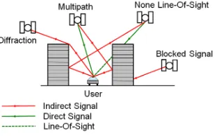
2.1.1 Sources of Error in GNSS While errors in the GNSS navigation solution calculation could arise from differences be-tween the true and broadcast ephemeris and satellite clock errors, as well as atmospheric issues and other sources, it is errors caused by blocked signals, Non-Line-of-Sight (NLOS) errors (which oc-cur when the direct signal is blocked and only a reflected signal is received), diffraction or Multipath that are specifically related to the 3D urban environment (Figure 1). These are explained in detail in (Groves et al., 2012).
Figure 1: Error in GNSS
2.2 Improving GNSS using 3D Modelling
A number of groups are working on using 3D city modelling to improve GNSS accuracy in urban areas. For example, (B´etaille et al., 2015) make use of highly simplified 3D models to distinguish between Line of Sight and NLOS satellite signals, and then com-pute corrections to pseudo-range measurements associated with the NLOS signals,creating additional “reliable signals” for inclu-sion in the positioning solution. (Suzuki and Kubo, 2013) and (Hsu et al., 2015) predict pseudo-range corrections using detailed 3D models. However, this is very computationally intense when a large number of candidate user positions must be considered.
2.2.1 Shadow MatchingThis uses a 3D city model to predict where within a street signals from each satellite can be directly received. Consequently, by determining whether a direct signal is being received from a given satellite, users can localize their position to within one of two areas of the street. By repeating this process for several different satellites, a position solution can be determined. Figure 2 illustrates this.
The Shadow Matching process firstly identifies a search area, per-haps by using conventional GNSS positioning techniques, and within this identifies a grid of candidate positions. For each posi-tion, the satellite visibility is predicted using the 3D City Model, by converting the model into a series of pre-computedBuilding Boundaries(see Section 4.2). Satelite elevations are compared with building boundary elevations at the appropriate azimuths, with the process repeated for each candidate position.
The pre-calculated availability values are then compared with the observed values (taking in to account the possibility of directly received or indirectly received signals) and (in a basic version of the algorithm) a score of 1 given for a match. The algorithm then calculates the final position by averaging the positions of the highest scoring candidates. Full details of this process are given in (Groves et al., 2015) and (Wang et al., 2015).
Within the above process, the 3D City Model is particularly im-portant when it comes to determining Building Boundaries (Sec-tion 4.2). During posi(Sec-tion determina(Sec-tion, each satellite eleva(Sec-tion is compared with the Building Boundary elevation at the same
azimuth. The satellite is predicted to be visible if it is above the Building Boundary. Thus the elevation point calculated for each azimuth is fundamental, as any error could result in a satellite being predicted as visible when it is not, or viceversa.
The results of real-world tests carried out using a mobile phone show an improvement in particular in the cross-street direction, with positioning error reduced from 14.81 m of the conventional solution to 3.33 m averaged across four test sites in London (Wang et al., 2013). More recent tests have recorded a reduction in mean positioning error across the street from 29.9m to 4.2m, while recording a slight increase in along-street mean error from 15.5m to 18.7m.
Figure 2: Principles of Shadow Matching (Groves et al., 2012)
2.3 Sourcing 3D City Models for Shadow Matching
Basic LoD 1 (i.e. with flat roofs (Kolbe et al., 2005)) 3D mapping can now be created cheaply and efficiently using the process of extrusion to grow 2D topographic mapping data to a given height, using information from, for example, Light Detection and Rang-ing (LiDaR) surveys where an aerial scan creates a cloud of points by illuminating the scene with a laser array and calculating the distance from the plan based on the reflection time.
More detailed (and realistic) 3D buildings are also becoming avail-able, either generated from individual Computer Aided Design (CAD) data, Building Information Models (BIM) or from terres-trial or airborne LiDaR using dense point clouds to ensure detail is captured. Although this type of detailed model tends to be available mainly for urban, city center, areas, these are in fact of great interest to Shadow Matching. These LoD 2 (i.e. with roof detail (Kolbe et al., 2005)) models may also be expensive, in particular where texture information is required.
In the UK it is now possible to obtain building height information for topographic mapping features for urban areas (via the Na-tional Mapping Agency (NMA), the Ordnance Survey), resulting in LoD 1 data. However, this data is expensive, and not univer-sally available in other countries.
An alternative approach, although very much in its infancy, is crowd-sourcing of 3D building information, where members of the public capture map data and contribute it to a shared database. 3D data capture currently forms part of OpenStreetMap’s world-wide mapping project (Over et al., 2010, Goetz and Zipf, 2012), which is described in (Haklay and Weber, 2008), and although 3D information is sparse at the moment, this approach shows promise for the future should it mirror the growth of the equivalent 2D Map.
dataset which is to be used for any extrusion process must be considered. Factors here include:
• What is the horizontal accuracy of the data?
• Is the data up to date and complete or are there missing buildings? Does the model include buildings under con-struction?
• Has the data been generalised at all, where generalization is the process of deriving a map or dataset with reduced complexity and contents from a detailed spatial data source, while retaining the major semantic and structural character-istics of the source data (Robinson et al., 1995).
• What has been modelled and to what level of detail - for example, what is the smallest feature captured? Does the 2D dataset include two polygons where a building has different roof levels? Are smaller details such as chimneys, trees and street furniture included as separate elements?
A second factor to consider is the quality of any LiDaR data used to determine the appropriate height for extrusion. Point density, in particular, is an important factor here as a low density (e.g. one point per 5m2) will result in a lack of candidate points for intersection with the building footprints, and hence accuracy in the resulting height information. Errors (incorrect measurements) in the LiDaR will also introduce errors in the City Model. There needs to be some level of correspondence between the chosen 2D topographic mapping and the point density, as even if small items such as chimneys are modelled in 2D, these are unlikely to be extruded to a correct height unless the LiDaR density allows the distinction of these objects from the surrounding roof structures.
3. DATA
The work described in this paper forms a part of a larger project (“Intelligent Positioning in Cities”) and the test area has been se-lected to allow comparison of results in an area where previous Shadow Matching tests have been carried out by the project team, and where there are known GNSS issues due to building config-uration - specifically, the area around Fenchurch Street in central London.
3.1 Topographic Mapping Data Sources
Three sources of topographic mapping data were used for this research, one of them (Ordnance Survey MasterMap) sourced via the UK’s EDINA service1 which provides access to a range of proprietary datasets for academic research, and the other two as open data2.
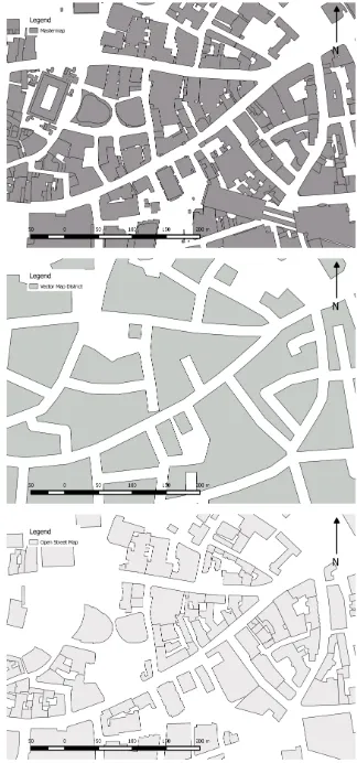
3.1.1 Ordnance Survey MasterMap (OSMM)Ordnance Sur-vey MasterMap provides highly detailed topographic mapping data for Great Britain, which also includes a height attribute for every building in major cities. The data is updated every six weeks, and has a capture scale of 1:1250 for urban areas3. The data has an absolute accuracy of 0.9m at the 99% confidence level with an RMSE of 0.5m4. All buildings over 8m2 are mapped5. Three height values are available for OSMM - the ground level, the base of the roof and the highest part of the roof and each height value is also accompanied by a confidence level which de-scribes the level of confidence in the accuracy of the height6. Fig-ure 3 (top) illustrates the data, which was last updated in January 2016.
1
http://edina.ac.uk/
2
Safesoft’s Feature Manipulation Engine (FME) software was used to create the datasets used for testing, and theQuickTranslatortool was used to load all data into PostGIS database http://www.safe.com/, Accessed 23rd May 2016.
3
https://www.ordnancesurvey.co.uk/test/products/topographylayer1.html, Accessed 23rd May 2016
4
https://www.ordnancesurvey.co.uk/test/products/topographylayer1.html, Accessed 23rd May 2016
5
https://www.ordnancesurvey.co.uk/docs/userguides/osMasterMaptopography-layeruserguide.pdf, Accessed 23rd May 2016
6
https://www.ordnancesurvey.co.uk/docs/collateral/products/buildingheight3d-modellingintro.pdf, Accessed 23rd May 2016
3.1.2 Ordnance Survey Vector Map District (VMD) Ord-nance Survey Vector Map District is an open dataset from the Ordnance Survey is designed to provide a “customisable back-drop map on which to pinpoint particular locations, show bound-aries and shaded-in areas”7. It also provides generalised 2D build-ings (amalgamated to block level) in vector format. The data is updated twice yearly, and is has a capture scale of between 1:15000 and 1:300008. Figure 3 (middle) illustrates the data, which was last updated in March 2016.
Figure 3: OS MasterMap (top) and Vector Map District (middle), OpenStreetMap (bottom)
3.1.3 OpenStreetMap (OSM)OpenStreetMap is a crowd sourced map with world wide coverage, which was initially created to ad-dress issues of data availability in the UK (Haklay and Weber, 2008) but has now grown to world-wide coverage. It has also been extended from a road network and an extensive set of points of interest, and now incorporates 2D building footprints, some of which also have associated height information. A number of sources have been used to create these maps including uploaded Global Positioning System (GPS) tracks, out of copyright maps and Yahoo! aerial imagery (Haklay and Weber, 2008). As the data is crowd-sourced, there is no single accuracy statement avail-able, and update frequency can vary. Research by (Koukoletsos et al., 2012) in 2012, examining the road network, has shown that OSM generally proves to be denser and more complete in the urban area (when compared to the Ordnance Survey MasterMap equivalent). However, research by (Fram et al., 2015) showed
7
https://www.ordnancesurvey.co.uk/businessand-government/products/vectormapdistrict.html, Accessed 28th May 2016
8
only a 33% completeness value for buildings in London, when compared to a vectorised version of OS Street View (which is an open 1:10k raster map9). Figure 3 (bottom) illustrates the data.
3.2 Sourcing Height Information
In order to extrude the VMD and OSM data to 3D, height data for the test area was sourced from the UK Environment Agency, who have recently published a 50cm resolution Digital Surface Model (DSM) which covers 70% of England, contains heights above sea level and is updated annually10. The data was trans-formed into a vector point dataset (for use in subsequent point in polygon calculations). Vertical height accuracy for the data is cited as: ±15cm11root mean squared error (RMSE), with more recent surveys falling to±5cm (RMSE quantifies the difference between the Ground Truth Survey and the LIDAR data). Hori-zontal error is cited as:±40cm12. The data is licensed under the Open Government License13.
3.3 Creating 3D Buildings
For the MasterMap data, a process of extrusion was then used to create three 3D datasets, using the base of the roof (OSMM Min) and maximum (OSMM Max) roof heights, as well as calculating their average (OSMM Avg). As both the VMD and OSM datasets do not have directly associated height values, the LiDaR dataset was used to identify heights for each building, using a point-in-polygon calculation as follows:
1. As the heights in the DSM are given above sea level, the first step in the process is to find the height above sea level at the base of each building. To allow for positional errors, all buildings were buffered to a distance of 5m, each buffer was given the ID of the associated building and then the buildings themselves used to cookie cut the buffers to that only the external buffer ring remained.
2. A point-in-polygon calculation was used to determine the average height of the DSM points in each buffer element, which is taken to be the best estimate of the height at the ground level of the associated building.
3. To determine the roof heights of the buildings, all the DSM points intersecting each building were identified, and the minimum, average and maximum height values calculated per building
4. The height at ground level for each building was then sub-tracted from these minimum, average and maximum values to give the local heights for each building
5. Each building was extruded to each of the three resulting heights (OSM Max, Avg and Min and VMD Max, Avg and Min).
6. Finally, the resulting datasets were converted to VRML for input into the Building Boundary creation process
3.4 Comparing the Datasets
Table 1 gives a brief comparison of the three datasets within the test area.
Metric OSMM VMD OSM
Number of Buildings 1295 99 483 Maximum Building Height 180 201 201 Minimum Building Height 1 22 9 Total Building Footprint (m2) 474287 579102 400460
Table 1: Dataset Comparison
9
https://www.ordnancesurvey.co.uk/business-and-government/products/os-streetview.html, Accessed 23rd May 2016
10
Further details can be found here: https://data.gov.uk/dataset/lidar-composite-dsm-50cm1, Accessed 23rd May 2016
11
http://www.geostore.com/environment agency/docs/Environment Agency LIDAR Open Data FAQ v5.pdf, Accessed 23rd May 2016
12
http://www.geostore.com/environment agency/docs/Environment Agency LIDAR Open Data FAQ v5.pdf, Accessed 23rd May 2016
13
http://www.nationalarchives.gov.uk/doc/open-government-licence/version/3/, Accessed 23rd May 2016
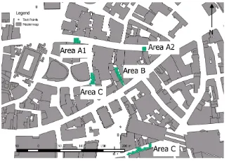
Overlaying the datasets as shown in Figure 4 reveals two issues - firstly, for the OSMM data, a number of buildings are miss-ing (circled in red on Figure 4 bottom). This may be due to the ongoing construction activities in the area and the rapid update frequency of OSMM (every 6 weeks). Secondly, the OSM and OSMM datasets are offset slightly (Figure 4 top) - this is due to a known transformation error when transforming the OSM data from WGS84 into British National Grid. A specific FME trans-formerBNGLatLongReprojector14was used for this purpose but did not totally resolve the issue.
Figure 4: OSMM/OSM (left) and OSMM/VMD overlay (right) showing missing buildings - OSMM buildings are shown with a thin black outline and no fill, VMD with a thick black outline
4. METHODOLOGY 4.1 Selecting the Grid Points
Building Boundaries are created for 360 1◦intervals around a
reg-ular set of grid points, which for the area in question around Fenchurch Street totals around 10,000 points (Section 4.2). Given the extensive amount of time required to generate one set of build-ing boundaries for this grid (over 24 hours), and as the focus of this paper is on the impact of individual building height variation rather than the impact over a large area, it was decided to test a subset of points in areas where building configuration provided an interesting contrast. Based on the recommendations of the GNSS experts, who have worked in this area for many years, the locations shown in Figure 5 were shown, resulting in a total of 121 distinct grid points, selected so as not to intersect buildings in any dataset. Specifically, Areas A1 and A2 were chosen to in-vestigate the impact of 3D data quality on a wide street, Area B is a narrow alleyway known as “Fenchurch Buildings”(15m wide, surrounded by buildings 50m high), Area C is in the shadow of the Leadenhall Building (143m in height) and “25 Fenchurch Av-enue” (61m height), Area D is close to Fenchurch Street Station, which is represented on the OSMM data but missing on OSM and VMD.
Figure 5: All 121 grid points tested, distributed over the area of interest around Fenchurch Street
4.2 Creating the Building Boundaries
A building boundary, which is a list of the elevation angles above which satellite signals become visible for a 360◦horizontal
ro-14
tation around a grid point, is determined at a number of differ-ent azimuths, spaced at regular intervals. For each azimuth, the building boundary is the highest elevation at which the LOS from a virtual satellite at that azimuth is blocked. This is determined using bisection: firstly the visibility of the virtual satellite at a 45◦elevation is tested. If it is blocked, the higher elevation region
is refined by bisection, and the next test is performed at an ele-vation of 45+45/2 = 67.5◦of elevation; otherwise, the satellite is
visible and the lower elevation region is refined, so the next test is at 45-45/2 = 22.5◦of elevation. The bisection process
contin-ues until the boundary has been determined to within 1◦elevation
resolution.
4.3 Comparing the Datasets: OSMM vs. OSM vs. VMD
To examine the impact of chosing between freely available data and data from an NMA, a comparison was made across all the grid points in the test dataset. To look at variation within each dataset, the first test calculated the maximum, minimum, aver-age, median, mode and standard deviation within the individual datasets. A second test took a comparative approach, subtract-ing the OSMM Avg and OSMM Min from OSMM Max and per-forming similar subtractions for the VMD and OSM datasets, as well as comparing both of these to OSMM.
4.4 Narrow Alleyway versus Wider Street
This examined the variability of values obtained in a narrow al-leyway with those obtained in a wider street. Narrow streets (in particular those surrounded by tall buildings) are particularly problematic for GNSS signal reception. This test was carried out on the OSMM dataset only, to eliminate the impact of missing buildings.
4.5 Cross Street Variation
Given that Shadow Matching provides accuracy improvements in particular in the cross-street direction, a third test focused on the variability of height values across a street, looking at both the nar-row alleyway (Area B) and the wider street (Area C). Elevation values for azimuth angles in both across street directions were compared, and the change in values across the street noted, to gain an understanding of the impact of varying building height at points close to the base of the building and further away.
4.6 Impact of Missing Buildings - Single Point Test
The final test in the series looked specifically at the impact of missing buildings near Area A1. An in-depth comparison of the values for one grid point was carried out, and a sky plot created to illustrate the variability in elevation results.
5. RESULTS
5.1 Comparing the Three Datasets: OSMM vs. OSM vs. VMD
5.1.1 Eliminating the OSM Min and VMD Min DatasetsA number of LiDaR points had negative elevation values, resulting in a negative minimum height for some of the extruded OSM and VMD buildings. As it was not possible to determine whether this was caused by deep excavations due to a construction process when the LiDaR survey took place, or by some other factor such as a glass roof over the buildings, OSM Min and VMD Min were eliminated from further evaluation.
5.1.2 Variation Within Each DatasetTable 2 shows the varia-tion of elevavaria-tion values within the individual datasets. As can be seen the variation in terms of the minimum and maximum eleva-tion values is considerable, reflecting the wide variaeleva-tion in build-ing heights in the test area.
As expected in an urban environment, the average elevation val-ues are relatively high. The minimum zero-valued elevation points correspond to a point on the map where there is a clear line of
OSMM
Min 0.00 0.00 0.00 0.00 0.00 0.00 0.00 Avg 64.55 67.47 69.79 56.70 71.95 57.37 64.96 Max 89.30 89.30 89.30 84.38 88.59 89.30 89.30 Med 70.31 73.13 75.94 61.88 77.34 66.80 74.53 Mode 79.45 80.86 81.56 67.50 80.16 82.27 86.48 StdDev 19.31 18.16 17.08 19.09 14.53 25.99 23.80
Table 2: Variation in Elevation Values for the Individual Datasets - Entire Test Area
sight - i.e. no obstructing buildings. In contrast, Figure 6 high-lights the point that results in the maximum elevation value of 89.30◦for OSMM - a grid point 0.2m away from a building.
Figure 6: Maximum elevation values for the OSMM dataset -point approximately 0.2m away from building
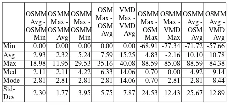
5.1.3 Variation Across the DatasetsTable 3 shows a compar-ison across the different datasets, highlighting the variation both within the different OSMM data and between OSMM, VMD and OSM. Min 0.00 0.00 0.00 0.00 0.00 -68.91 -77.34 -71.72 -57.66 Avg 2.93 2.32 5.24 7.59 15.25 4.83 -2.16 10.10 10.78 Max 18.98 11.95 29.53 35.16 40.08 88.59 85.08 88.59 84.38 Med 2.11 2.11 4.22 6.33 14.06 0.70 0.00 4.92 9.14 Mode 2.81 2.81 2.81 2.81 14.06 0.70 2.81 2.81 8.44
Std-Dev 2.30 1.77 3.95 5.75 7.87 24.53 12.43 25.67 12.89
Table 3: Variation in Elevation Values Comparing Datasets - En-tire Test Area
Examining the situation on the ground where the maximum varia-tion occurs between the elevavaria-tion for the OSMM Max and OSMM Min datasets. This 29.53◦variation corresponds to a building
hav-ing maximum height of 41.6m and minimum height (at the eaves) of 13.2m. Figure 7 illustrates the maximum variation between OSMM Max and OSM Max - i.e. 88.59◦. This is caused by a
missing building in the OSM dataset.
5.2 Narrow Alleyway versus Wider Street
This test compared 27 points in Leadenhall Street (Areas A1 and A2) with 29 points in Fenchurch Buildings (Area B). Ta-ble 4 shows the results obtained. As expected, the narrower area yielded higher average and maximum elevation values. However, the variation in maximum elevation value caused by the differing OSMM heights is only 0.7◦in the wider street, and 0◦in the
nar-row alleyway, with the average values varying by 3.94◦for
Figure 7: Maximum Variation between OSMM Max and OSM Max heights showing OSM (left) and OSMM (right) with the blue rays representing the elevations for the OSMM Max height data, and the black for the OSM Max data
OSMM Min Leaden-hall
OSMM Avg Leaden-hall
OSMM Max Leaden-hall
OSMM Min Fenchurch Blds
OSMM Avg Fenchurch Blds
OSMM Max Fenchurch Blds Min 0.00 0.00 0.00 14.77 15.47 18.28 Avg 58.75 60.81 62.69 72.45 75.02 76.95 Max 87.89 87.89 88.59 89.30 89.30 89.30 Med 64.69 66.80 68.91 76.64 78.75 80.16 Mode 72.42 71.72 73.13 82.97 85.08 85.78 Stdev 21.09 20.67 20.12 14.17 12.66 11.42
Table 4: Variation in Elevation - Wide Street (Leadenhall, Area A) versus Narrow Alleyway (Fenchurch Buildings, Area B)
5.3 Cross Street Variation
Azimuth OSMM Min
OSMM Avg
OSMM Max
VMD Avg
VMD MaxOSM Avg
OSM Max 0 66.80 71.02 74.53 62.58 78.05 64.69 78.75 0 72.42 75.94 78.75 68.20 80.86 31.64 47.81 0 78.75 81.56 82.97 74.53 83.67 33.05 49.22 0 85.78 86.48 87.19 80.86 85.78 34.45 50.63 180 87.89 87.89 88.59 82.27 85.08 7.03 10.55 180 74.53 77.34 78.75 72.42 78.75 6.33 9.84 180 80.16 82.27 83.67 77.34 82.27 6.33 10.55 180 69.61 72.42 75.23 67.50 75.94 6.33 9.84
Table 5: Variation in Elevation Across the Three Data Sources North/South Across the Street - Clutched Friars
Table 5 shows the cross-street variation for four points in Area C, close to the station, for 0 and 180◦Azimuth. There is a
sig-nificant difference from one side of the street to another - with a variation of 15.47◦, for example, for the OSMM Avg dataset.
Table 6 shows a similar variation across the street in Area B, and as expected the corresponding variation for the OSMM Avg data is lower, given the height of the surrounding buildings and the narrowness of the street. Figure 8 illustrates the variation. Com-paring OSMM Max and VMD Max yields a variation of -3.52, -2.11, -0.70 and 1.41◦across the street for the 0◦azimuth for Area
A. Similarly, for Area B, at azimuth 90, variations of 5.63, 2.11 and 3.52◦are observed.
Azimuth OSMM Min
OSMM Avg
OSMM Max
VMD Avg
VMD MaxOSM Avg
OSM Max 90 84.38 85.78 86.48 68.91 80.86 87.89 88.59 90 72.42 75.23 77.34 56.25 75.23 71.72 78.75 90 78.05 80.16 81.56 62.58 78.05 79.45 83.67 270 73.83 75.94 77.34 66.80 80.16 73.13 76.64 270 80.86 82.27 82.97 73.83 82.97 79.45 81.56 270 87.89 87.89 88.59 80.86 86.48 86.48 87.19
Table 6: Variation in Elevation Across the Three Data Sources East/West Across the Street - Fenchurch Buildings
5.4 Impact of Missing Buildings - Single Point Test
Figure 10 illustrates the location of the point selected for this test - as can be seen both the VMD and OSM datasets have missing buildings. As shown on the sky-plot (Figure 9) this results in a very high variation in elevation values for the same point. While the three OSMM datasets follow a consistent pattern around the 360◦of the plot (varying by only a few degrees) there is
mini-Figure 8: Fenchurch Buildings - Variation Across the Street
mum variation of -75◦between OSMM Max and VMD Max,
in-dicating that the VMD Max value is high where the OSMM Max value is low. This corresponds to the 300◦azimuth angle, which
is characterized by an extended corner (created by the general-ization process) on the VMD building in contrast to the smooth corner on OSMM. A similar issue can be seen at 270◦azimuth
(i.e. due west) where the ray will intersect the OSMM build-ing, with an angle of 76.64◦for OSMM Max, yielding 55.54◦for
VMD (due to the building further away to the left) and 4.92 for OSM as there are no close buildings west of the point (there is a building further away, as can be seen in the smaller scale map in Figure 3).
Figure 9: Skyplot showing the variation in elevation values around a single point (Point A1, Figure 10)
6. DISCUSSION
The work described in this paper shows that it is possible to generate 3D city models for London using open data, in par-ticular given the availability of very high density LiDaR points. As could be expected, the differing heights within the OSMM dataset yielded relatively small incremental increases in eleva-tion value in most cases, although the maximum difference of 29.53◦is noteworthy. The variations when comparing the
eleva-tion values created using the different datasets are more signifi-cant, with maximum values around the 85-88◦, caused by
miss-ing buildmiss-ings. Cross street variation, of particular interest to the Shadow Matching process, confirms that the impact of height differences is greater when the grid points are closer to particu-larly tall buildings, yielding a difference of 7.73◦for OSMM Max
and OSMM Min close to the wall in Area B, with only 4.22◦in
the middle of the street. A similar effect was observed in the narrow street surrounded by tall buildings, with a variation of 4.50◦between OSMM Max and OSMM Min.
The results obtained highlight the importance of developing a good understanding of the quality underlying 3D city model, and its behaviour within the specific algorithm in which it is to be used - in this case the Building Boundary creation algorithm that calculates the relevant elevation values at which a GNSS satel-lite is visible from a specific point. The impact on the results of the varying quality of the 3D datasets tested is discussed in more detail here.
6.1 Availability of 3D City Models
Three different 3D datasets were used to create the models above, two of which have been created using open data sources. Al-though the skills required to do this are perhaps not widespread outside the GIS community, and the method used was relatively simplistic (taking average LiDaR point heights within a build-ing polygon, usbuild-ing a point-in-polygon algorithm), the approach does show the potential to create an open 3D LoD 1 dataset for London, where to date one does not exist. This approach could also be deployed in other cities, permitting wider deployment of Shadow Matching. The availability of such a dataset may in turn increase the uptake of 3D GIS.
6.2 Using LiDaR for Heighting Buildings
The algorithm used to determine building heights caused issues with the minimum height values for roof structures of the OSM and VMD buildings (perhaps due to a deep construction site at the time of survey). Access to corresponding imagery for the area of interest would be helpful here, as this could be confirmed and the negative values eliminated from the ground height determina-tion process. The assumpdetermina-tion of uniformity of the roof structure and the assumption of which points are at ground level could also impact the results obtained. For the former, the presence of a small but high chimney will give rise to an exaggerated maxi-mum height value for the roof, whereas in reality the chimney would only block a few of the satellite signals to the grid points. This means in turn that the grid points will show lower satellite availability in reality. For the latter, the presence of cars or other structures on the street within the 5m buffer of the building could yield a higher ground height than in reality, resulting in a lower overall building height and an hence lower elevation values and a model that shows higher satellite availability than in reality.
6.3 The Impact of Generalisation
Figure 3 highlights the generalised nature of the VMD dataset, which contains 104815m2 of building footprint more area than the OSMM data (the total test area is approximately 776900m2), with a consequent loss of potential grid points for Building Bound-ary generation. Generalised data also has consequences in terms of the extrusion process using the LiDaR data as points that are in
reality on the ground may appear to be on a roof surface, resulting in lower average height values. This is reflected in Table 2, which shows that while the maximum elevation angle for the VMD Max dataset is close to that of OSMM (88.59 and 89.30◦respectively)
the average angles are 84.38◦versus 89.3◦for OSMM.
6.4 The Impact of the Grid Points Configuration
The grid points used for the tests described above are spaced at 3m intervals, and aligned to the integer coordinate values on the British National Grid projection. Grids are oriented North/South no matter the direction of the street and hence the surrounding buildings. Thus, they do not truly represent the space in which they are located, with some grid points located unrealistically close to buildings (Figure 6). This requires the Shadow Match-ing system to store and process data which in practice is perhaps never used as a hand-held GNSS device is unlikely to be that close to a building.
6.5 The Impact of Missing Buildings
Parts of the test area for this paper are undergoing redevelopment, making it difficult to keep the mapping data current, as can be seen by the number of instances where buildings appear in one dataset and not in another. Absent buildings (or the presence of buildings that in reality are not there) have the greatest impact on the Building Boundary results, highlighting the importance understanding the completeness and currency of the data that is being used, and ensuring it is updated on a frequent basis.
6.6 Crowd Sourced and NMA Data
The OSMM dataset specification clearly describes the minimum building footprint included in the model, as well as assigning a level of confidence to the height value. The LiDaR data from the Environment Agency also includes a vertical height accuracy value and the VMD dataset has a nominal capture scale. Up-date frequencies of the datasets are known. These measures al-low GNSS experts to understand whether the 3D dataset is fit-for-purpose and gauge the reliability of the resulting elevation values. Horizontal positional accuracy values are not, however, available for the crowd-sourced OSM data, and the unresolved shift between the OSM and OSMM dataset is further cause for concern. It would also be useful to know the minimum modelled building size and whether features such as chimneys are modelled separately, given their potential impact on overall roof height. In some cases, a crowd-sourced dataset may in fact be more up-to-date than an “official” dataset as it is maintained by people living or working in the neighbourhood, who observe and map changes as they happen. However, overall quality is difficult to determine without studying both the update history of the dataset (which is available should this be required) and perhaps the behaviour of the specific individuals capturing the data - are they trusted by the wider community to create high quality maps?
7. CONCLUSION AND FURTHER WORK
and thus determine the minimum horizontal and vertical accu-racy, currency and building footprint requirements for a 3D city model for Shadow Matching. In particular, observing the dif-ference that using the three different height values for OSMM makes could provide useful insight as to whether it is better to over-estimate satellite availability by using the lowest height or to underestimate by using the highest. To add to this evaluation, the datasets created above were all LoD1. However the availabil-ity of higher densavailabil-ity LiDaR points - the Environment Agency has also released 25cm LiDaR density - gives the potential to create a relatively accurate LoD 2 dataset with city-wide coverage rather than the individual buildings mentioned in Section 2.3. Other fac-tors to be explored including the reflectivity of building surfaces which, as noted in Section 2.1.1, can cause multi-path errors. The focus of the work described in this paper was on the im-pact of 3D data quality on GNSS signal modelling but also have implications for other types of signal propagation in an urban en-vironment - e.g. for radio and mobile phones. At a broader level, further work remains to be done on the 3D data itself, to develop a suitable approach to compare the quality, and particularly the building heights derived from the LiDaR data, with ground truth data. To address the absent buildings issue (and hence the cur-rency of the dataset) it may be possible to add a measure of un-certainty to the data, so that the elevation values are tagged with an accuracy weighting (similar to that described for OSMM in Section 3.1.1). This may be derived by comparing two datasets where these are available - in this case OSM and VMD (given the high cost of OSMM). The LiDaR data may also provide a use-ful indication as to the location of missing buildings, as above-ground points should correspond to building footprints. Given that the OSM data is crowd-sourced, it is also important to under-stand whether update frequency, or the number of updates on a particular building, reflects the quality of the data , using similar approaches to those currently used for OSM road network data (Haklay et al., 2010).
The current Building Boundary creation process makes use of a systematic rotation of 360◦around a point, and calculates the
required elevation by a process of bisection and ray-generation. Given that 3D intersection functionality exists in spatial databases, it may be possible to take advantage of spatial indexing to only intersect the rays with buildings that are closest to the grid point, reducing the number of candidate buildings for intersection and hence improving the efficiency of the process. GIS may also prove useful in generating more realistic grids of points for use in the Shadow Matching algorithm, for example by orienting the grid along the direction of the street, and ensuring that each point is at minimum 1m from a building.
Coupled with the processes described above, further understand-ing of the positional accuracy required for the applications of GNSS in urban areas mentioned in Section 1 is required, in par-ticular in the across street direction where Shadow Matching pro-vides best improvements, with the aim to deploying a useful real-world solution. The increased ability to model accurate user lo-cations within the urban environment, provided by more detailed 3D city models and a better understanding of how their quality impacts the accuracy of the positioning results, will help achieve this goal.
ACKNOWLEDGEMENTS
All maps in this paper contain OS data cCrown copyright and database right (2016). This work forms part of the Intelligent Po-sitioning in Cities project, which is funded by EPSRC (EP/L018446/1).
REFERENCES
Bauer, C., 2013. On the (In-) Accuracy of GPS measures of Smartphones: a study of running tracking applications. In: Pro-ceedings of International Conference on Advances in Mobile Computing & Multimedia, ACM, p. 335.
B´etaille, D., Peyret, F. and Voyer, M., 2015. Applying Stan-dard Digital Map Data in Map-aided, Lane-level GNSS Location. Journal of Navigation 68(05), pp. 827–847.
Ellul, C., Gupta, S., Haklay, M. M. and Bryson, K., 2013. A Platform for Location Based App Development for Citizen Sci-ence and Community Mapping. In: Progress in Location-Based Services, Springer, pp. 71–90.
Fram, C., Christopolou, K. and Ellul, C., 2015. Assessing the quality of OpenStreetMap building data and searching for a proxy variable to estimate OSM building data completeness. GIS Re-search UK (GISRUK) 2015 Proceedings.
Goetz, M. and Zipf, A., 2012. OpenStreetMap in 3D–detailed insights on the current situation in Germany. In: Proceedings of the AGILE 2012 International Conference on Geographic Infor-mation Science, Avignon, France, Vol. 2427, p. 2427.
Groves, P. D., 2013. Principles of GNSS, inertial, and multisensor integrated navigation systems. Artech House.
Groves, P. D., Jiang, Z., Wang, L. and Ziebart, M. K., 2012. Intel-ligent Urban positioning Using Multi-Constellation GNSS with 3D Mapping and NLOS Signal Detection. Proceedings of ION GNSS.
Groves, P. D., Wang, L., Adjrad, M. and Ellul, C., 2015. GNSS Shadow Matching: The Challenges Ahead. Proceedings of the 28th International Technical Meeting of The Satellite Division of the Institute of Navigation.
Haklay, M. and Weber, P., 2008. OpenStreetMap - User Gener-ated Street Map. IEEE Pervasive Computing pp. 12–18.
Haklay, M., Basiouka, S., Antoniou, V. and Ather, A., 2010. How many volunteers does it take to map an area well? The validity of Linus law to volunteered geographic information. The Carto-graphic Journal 47(4), pp. 315–322.
Hsu, L.-T., Gu, Y. and Kamijo, S., 2015. NLOS Correc-tion/Exclusion for GNSS Measurement using RAIM and City Building Models. Sensors 15(7), pp. 17329–17349.
Kolbe, T. H., Gr¨oger, G. and Pl¨umer, L., 2005. CityGML: In-teroperable access to 3D city models. In: Geo-information for disaster management, Springer, pp. 883–899.
Koukoletsos, T., Haklay, M. and Ellul, C., 2012. Assessing data completeness of VGI through an automated matching procedure for linear data. Transactions in GIS 16(4), pp. 477–498.
Over, M., Schilling, A., Neubauer, S. and Zipf, A., 2010. Gen-erating web-based 3D City Models from OpenStreetMap: The current situation in Germany. Computers, Environment and Ur-ban Systems 34(6), pp. 496–507.
Robinson, A. H., Morrison, J., Muehrcke, P. C., Kimerling, A. and Guptill, S., 1995. Elements of Cartography. John Wi-ley&Sons Inc., New York, USA.
Suzuki, T. and Kubo, N., 2013. Correcting GNSS Multipath Er-rors using a 3D Surface Model and Particle Filter.
Wang, L., Groves, P. D. and Ziebart, M. K., 2013. Urban Po-sitioning on a Smartphone: Real-Time Shadow Matching Using GNSS and 3D City Models. Proceedings of the 26th Interna-tional Technical Meeting of The Satellite Division of the Institute of Navigation.
Wang, L., Groves, P. D. and Ziebart, M. K., 2015. Smartphone Shadow Matching for Better Cross-Street GNSS Positioning in Urban Environments. Journal of Navigation 68(03), pp. 411–433.