MONTE-CARLO-SIMULATION FOR ACCURACY ASSESSMENT OF A SINGLE
CAMERA NAVIGATION SYSTEM
F. Bethmann a, T. Luhmann a
a Jade University of Applied Science Oldenburg, Institute of Applied Photogrammetry and Geoinformatics, Ofener
Straße 16-19. 26121 Oldenburg, Germany –folkmar.bethmann@jade-hs.de, luhmann@jade-hs.de
Commission V, WG V/1
KEY WORDS: Medicine, 6DOF- Navigation, Monte-Carlo- Simulation, Single camera solutions, Accuracy assessment
ABSTRACT:
The paper describes a simulation-based optimization of an optical tracking system that is used as a 6DOF navigation system for neurosurgery. Compared to classical system used in clinical navigation, the presented system has two unique properties: firstly, the system will be miniaturized and integrated into an operating microscope for neurosurgery; secondly, due to miniaturization a single camera approach has been designed. Single camera techniques for 6DOF measurements show a special sensitivity against weak geometric configurations between camera and object. In addition, the achievable accuracy potential depends significantly on the geometric properties of the tracked objects (locators). Besides quality and stability of the targets used on the locator, their geometric configuration is of major importance. In the following the development and investigation of a simulation program is presented which allows for the assessment and optimization of the system with respect to accuracy. Different system parameters can be altered as well as different scenarios indicating the operational use of the system. Measurement deviations are estimated based on the Monte-Carlo method. Practical measurements validate the correctness of the numerical simulation results.
1. INTRODUCTION
1.1 State-of-the-art: 6DOF navigation in clinical surgery
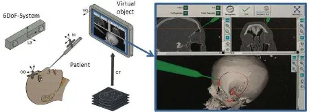
In computer-assisted surgery (CAS) complex image-based navigation system are used for years that provide an assistive tool for the surgeon for planning and performing of operations. Their main objective is the application of minimal invasive operations and the minimization of health risks. Image-based navigation systems allow for the continuous measurement of the six degrees of freedom (6DOF) that define the relative position and orientation between human patient and medical tools (e.g. surgical instruments). The measurement 3D information can be combined with planning data as they are available from pre-operatively acquired CT or MRT imagery. Figure 1 displays an overview of the components of an image-based navigation system. Depending on the clinical application different systems are used for 6DOF tracking. Among them are mechanical sensors, ultra-sound systems, electromagnetic systems and optical systems whereby the latter two are most established in practice (Birkfellner, 2011).
Figure 1. Image-based navigation (after Birkfellner, 2011)
Electromagnetic systems benefit from the fact that no free visual sighting is required between surgical instrument (sensor unit)
and measurement system (emitter). As a drawback they are extremely sensitive to external error sources, e.g. electromagnetic fields of other devices, interferences or occlusions by metal objects. Enhanced approaches for system calibration can reduce the effect of error sources (Krüger et. al., 2009). However, achievable measurement accuracies lie in the order of up to 1cm in a measurement volume of 500 x 500 x 500 mm (Weyhe & Broers, 2009), hence they are significantly worse than optical systems with accuracies in the sub-millimeter domain (Broers & Jansing, 2007).
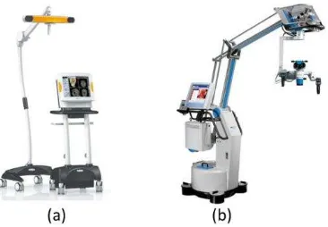
Optical navigation systems used in medical applications are usually designed as stereo camera systems using a fixed mounting of two cameras on a stable base. Normally they are applied as stand-alone systems to be positioned next to the operation table (Figure 2a). Thus several problems arise by occlusions or restricted field of view in those medical areas where particular narrow environments are given, e.g. for neurosurgery or otolaryngology.
1.2 Microscope-integrated optical navigation
Based on the above mentioned situation a joint project between Möller-Wedel (Hamburg), AXIOS 3D, OFFIS and IAPG (all Oldenburg, Germany) has been established for the development of a single camera 6DOF tracking system to be used in an operating microscope (Figure 2). This concept allows for the simultaneous guidance of microscope and navigation system to the field of interest enabling free sight to the operational area and all relevant surgical tools. Integrating the camera into the microscope offers additional benefits, e.g. improved geometric conditions by reduced observation distances, and simplification of the technical solution (no need for high precision stability of two cameras).
Up to now the use of single camera 6DOF solutions and the integration of navigations into a microscope are rarely applied in clinical navigation. The only known version of integrated navigation is presented by electromagnetic systems (Fiagon, 2012) offering the above mentioned disadvantages.
Figure 2. a) Stereo system (Brainlab, 2011), b) operation microscope (Möller-Wedel, 2011)
1.3 Microscope-integrated optical navigation
Applying 6DOF navigation with a single camera comes along with a high sensitivity against weak geometric configurations between camera and object (Luhmann, 2009, Suthau, 2006). This fact is problematic for the desired system since hand-held surgical tools require a high flexibility in terms of spatial position and orientation. Luhmann (2009) has shown that the quality of 6DOF measurement using a single image can be improved if the spatial distribution and accuracy of locator targets is optimized. The desired accuracy of locator position in this project is specified to 2-3 mm for the superimposition of locator position with CT or MRT imagery. For this reason a numerical simulation is used to investigate different system designs and to optimize the achievable measurement accuracy. In addition, possible limit cases (critical imaging configurations) shall be identified.
The following section describes the measuring system and the measurement process for 6DOF navigation. In section 3 the Monte-Carlo based simulation approach for estimation of the theoretical measurement precision is presented. Section 4 discusses system investigations and solutions for system optimization.
2. MEASUREMENT SYSTEM AND PROCESS
Single image 6DOF measurement is based on the observation of two or more point fields (locators) that are fixed to the objects to be tracked. For the developed system each locator consists of five control points which are designed as flat or spherical retro-reflective targets. Four of the five points lie within a common plane. The local coordinates of the control points are calibrated in advance. The reference locator (XR, YR, ZR) is mounted in a fix position at the patient while the probing locator (XL, YL, ZL) represents the surgical instrument (Figure 3). The spectral sensitivity of the camera is limited to near infrared, hence an adapted illumination unit (infrared flash) yields to high contrast image points without disturbing background information. The camera will consist of a 776 x 582 pixel sensor and a 4mm lens.
Figure 3. Coordinate systems of single image navigation
The goal of 6DOF tracking is the determination of the six transformation parameters that form the spatial position and orientation of the probing locator with respect to the coordinate system of the reference locator (transformation T3, see Figure 3). The calculation of the transformation parameters is based on the exterior orientation of the camera derived from measured image coordinates of the control points of the reference locator (XR, YR, ZR) and the control points of the probing locator (XL, YL, ZL). The interior orientation (camera calibration) is assumed to be known. Image points are measured by ellipse operators.
The parameters of exterior orientation can be used to determine two translation vectors (X0R and X0L defining the position of the perspective center in systems XR, YR, ZR and XL, YL, ZL) and two rotation matrices (RR and RL defining the orientation of the camera in systems XR, YR, ZR and XL, YL, ZL). The desired transformation T3 of a point x from the probing system into the reference system is given by:
Refer to (Luhmann, 2009) for a complete derivation of formula (1). In order to transform the orientation data into the system of the CT or MRT (XCT, YCT, ZCT), an additional transformation T4 is necessary. The required transformation parameters are determined independently in a separate image-to-patient registration process. This task is a complex process (Eggers, 2011) and will not be considered in the following investigation.
3. MONTE-CARLO SIMULATION
Using a simulation program the measurement errors of the system as a function of different virtual system prototypes and imaging configurations will be analyzed. The analysis is based on the Monte-Carlo method (Metropolis & Ulam, 1949) which is widely used in metrology. Example applications are presented by Wäldele et al. (2005) for coordinate measurement machines or Hastedt (2004), Broers & Jansing (2007) and Luhmann (2009) in the field of photogrammetry.
Monte-Carlo simulation requires the known relationship of all result values with respect to their input parameters in terms of mathematical or algorithmic functions. In addition, the error or noise distribution of all input values can be defined appropriately by statistical probability functions. The computation of the simulation is performed on a number n of virtual experiments where all input parameters are altered according to their statistical distribution. As a result n output values are calculated that vary with respect to the noisy input data. The analysis of the resulting values can be done directly in comparison to error-free reference values that can be derived from undistorted input data.
The histogram of (Figure 4a) illustrates the empirical distribution function of the resulting value which can be used to derive confidence intervals (e.g. standard error for factor k=1, probability 68.3%). For this investigation the accuracy of 3D coordinates of selected probing points in the reference coordinate systems are of major interest. The resulting Monte-Carlo values can be visualized as graphical confidence ellipsoids (Figure 4b) which can be extracted from the variance-covariance matrix (Niemeier, 2002).
Figure 4. Presentation of results: histograms (a), 3D confidence ellipsoids (b)
In the first implementation of the Monte-Carlo simulation program Gaussian distributed random noise is applied to the following input values:
image coordinates (x'i, y'i)
3D coordinates of control points of the probing locator (XLi, YLi, ZLi)
3D coordinates of control points of the reference locator (XRi, YRi, ZRi)
interior orientation parameters according to photogrammetric standard model (ck, xh, yh, A1, A2, A3, B1, B2, C1, C2)
For the practical use of the system systematic errors may occur, mainly caused by disturbed or occluded targets. It is the objective of future developments to enhance the current simulation program to build a 'virtual measuring machine'(Schwenke et al., 2000). Therefore additional systematic effects have to be modeled and introduced into the calculation. Recently systematic errors are not yet considered.
4. VALIDATION OF MONTE-CARLO SIMULATION
For the validation of the simulation model real measurements will be carried out that allow for a comparison of the coordinates of the locator's probing tip with respect to reference data of higher accuracy. The test will also include an analysis of the correctness of simulated confidence intervals in order to test the assumptions that have been introduced into the Monte-Carlo simulation.
4.1 Test object
The test object used for the following investigation represents a static measurement situation with a fix configuration of reference and probing locator points on a common aluminum plate (Figure 5). The target points are located within Hubbs nests that permit the measurement with a laser tracker probing ball and photogrammetric retro-targets as well.
Figure 5. Test object
In order to create reference data of higher accuracy the 3D coordinates oft he targets are measured by a laser tracker (API Tracker 3). Laser tracker measurements have been repeated three times in a weekly interval. The maximum point error yields ∆rXYZ = 11 µm. During reference measurements the room
temperature was stabilized to ∆T = +/- 1.5°K. Assuming a thermal coefficient of α = 23.0·10-6 K-1 for aluminum a maximum length change ∆L = 24 µm for the longest dimension of the plate (L = 350 mm) can be estimated.
The coordinates are determined in a common coordinate system (XL = XR, YL = YR, ZL = ZR) with its origin in the probing tip (Figure 5). This enables a simple generation of nominal values of the result, since both locators are given in the same coordinate system: XT=YT=ZT=0.0 [mm] (coordinates of probing tip in reference system).
4.2 Test scenarios and results
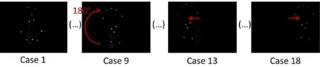
Within a series of tests 18 static imaging configurations have been investigated. The camera used is an AXIOS 3D SingleCam C8 (f = 8 mm, 776 x 582 pixels, pixel size: 8.3µm x 8.3µm). The camera has been calibrated using a photogrammetric standard distortion model. The optical axis is directed perpendicular to the XY-plane of the test object for all 18 scenarios. Imaging distance amounts to ca. 800 mm leading to a pixel size in object space of about 0.8 mm. The test object is rotated step by step in a 180° range and shifted so that the object is visible in the left and right image area. Figure 6 shows image examples for the scenarios 1, 9, 13 and 18.
Figure 6. Test scenarios 1, 9, 13, 18
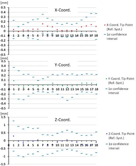
In each test scenario approximately 1000 images have been taken and processed. It is assumed that the average of these 1000 measurements is almost free of random errors, hence is only affected by systematic errors. These deviations are displayed in Figure 7 for all 18 tests (X-, Y-, Z-coordinates of probing tip).
For the validation of the Monte-Carlo approach simulations have been calculated for all test scenarios based on the real imaging configurations. For this purpose the average exterior orientation values of the camera are introduced to the simulation.
Figure 7. Measured values of probe coordinates and simulated confidence intervals
The introduced standard deviations rely on a priori known typical values. The standard deviation of image points measured by ellipse operator can be estimated to sx’y‘ = 0.05 pixel while the standard deviation of control points is assumed to be sXYZ = 0.075 mm. The standard deviations for interior orientation parameters are taken from bundle adjustment results for camera calibration (sc = 0.0003 mm, sxo = 0.008 mm, syo = 0.008 mm, sA1 = 1.8·10
-5
mm-2, sA2 = 2.9·10 -6
mm-4, sA3 = 1.4·10-7 mm-6, sB1 = 5.0·10-6 mm-1, sB2 = 5.0·10-6 mm-1, sC1 = 1.1·10-5, sC2 = 1.0·10-5). 3000 simulation iterations have been calculated for each scenario in order to compute standard deviations of the probing tip coordinates. They lead to 1σ -confidence intervals that are illustrated in Figure 7.
Analyzing the simulation results it becomes obvious that empirical confidence intervals could be derived that cover the reference value in all cases. Therefore the introduced noise values will further be used for the subsequent step of system optimization.
5. SYSTEM OPTIMIZATION
The process of system optimization consists of the variation of imaging properties of the camera (focal length, distortion parameters) and the variation of locator designs. Due to practical reasons the variations must be limited to available equipment and ergonomic conditions. Therefore a camera with 4mm focal length has been used because the future system will consist of a similar lens. In addition the design of the reference locator will be kept fixed in order to limit the number of possible scenarios. The main objective of the optimization process is the optimal design of the probing locator.
5.1 Probing locator designs
Table 1 shows a number of locator point designs that result from a longer development process including specific measurement criteria and ergonomic aspects.
Table 1. Probing locator designs
Ergonomic aspects are of high importance since the surgical instruments should not result in extended physiological and cognitive impacts for the working surgeon. Acceptance or rejection of systems in clinical environments is significantly influenced by ergonomic properties of the product. The illustrations in Table 1 show a view to the XY plane of the probing locator. In principle the point positions vary in Y direction (locator width), the position and Z value of the outstanding point and the distance of the point field to the locator tip.
From a metrological point of view it can be expected that an enlarged volume of locator point distribution and a reduced distance to the probing tip will enhance the measurement accuracy (Lange & Schlag, 2011, Eggers, 2011). In order to optimize the locator design according to ergonomic aspects, a contrary approach is recommended. The layouts of Table 1 illustrate this conflict. Variants 1 and 2 are optimized with respect to ergonomic handling due to their small size (∆Y = 6.0 mm) and the low outstanding point (∆Z = 10.0 mm). They differ only in the position of the outstanding point. In variant 1 the outstanding point is located in front area in order to avoid point occlusions of the other points if the locator is tilted. For variant 2 the outstanding point is located in the center of the plane points. Variant 3 enlarges the locator size in Y direction
(∆Y = 12.0 mm). The same idea is valid for variant 4 whereby the dimension is limited to ergonomically accepted values
(∆Ymax = 35.0 mm), reducing the width of the locator in direction to the probing tip. Another difference between 3 and 4 is the enlarged point distance in X (from ΔX = 53 mm to ΔX = 70 mm) and the increased Z value of the outstanding point (∆Z = 20 mm). For variant 5 the complete point field is shifted towards the probing tip.
5.2 Test scenarios
The simulation program enables the computational representation of different scenarios in order to analyze the impact of locator movements (e.g. successive rotations and translations) systematically. The measurement space is formed
Locator 1 Locator 2 Locator 3 Locator 4 Locator 5
by a defined number of discrete object points that are arrange grid-wise in a cylindrical volume. For the following investigations a total number of 45 object points are created that lie in three spatial planes with different distances to the camera (Figure 5, A: side view, B: ground view).
Figure 8. Imaging configurations
Each object point is 'probed' by simulation using 18 different probing locator orientations. Each rotation angle ω, φ, κ is altered in six steps within the intervals –45.0° < ω < 45.0°,
–45.0° < φ < 45.0° und –90.0° < κ < 90.0°. The angle describe the rotation of the probing locator with respect to the camera coordinate system x', y', z'. The spatial distribution of the reference locator points is identical for all tests. It forms a half circle with five object points as it will be used in practical operation (Figure5 C).
5.3 Monte-Carlo simulation
Due to the 18 probing of all 45 object points each locator design is tested in a total of 810 scenarios. Each scenario is computed by n = 3000 simulation iterations where all input parameters are modified by noise according to
1
z
s
P
P
v
P
(2)
(with P: input parameter, Pv: modified input parameter, sP: standard deviation of input parameter, z1: Gaussian random number). The standard deviations have been selected according section 4.2.
5.4 Results
The achievable accuracy is analyzed by the deviations of the probing tip position according to equation (1). The interval of the deviation is defined by the standard deviations sX, sY, sZ given in the reference coordinate system. They have been calculated 18 times for each measured point.
Figure 9. Maximum and mean (black line) standard deviations
Figure 9 displays the maximum and mean standard deviations resulting from all scenarios in order to analyze the performance for the complete measurement volume and all probing strategies.
It becomes clear that the point variations of Table 1 lead to a significant improvement of accuracy. The mean standard deviations are reduced from sXY≈ 0.5 mm and sZ≈ 2.4 mm for locator 1 to sXY≈ 0.15 mm and sZ≈ 0.75 mm for locator 5. The maximum standard deviations are reduced from sXY≈ 1.15 mm and sZ≈ 4.0 mm to sXY≈ 0.30 mm and sZ≈ 1.30 mm.
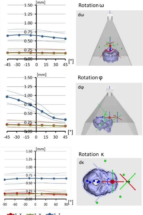
Figure 10 displays the deviations as a function of probing direction angle showing mean (solid lines), minimum and maximum (dashed lines) standard deviations for locator design 5. It is obvious that the extremes of mean and maximum standard deviations in Z are mainly depending on angle φ. The largest deviations are achieved at φ = –45° which is identical to
φmin in the center image of Figure 10. The standard deviations in X and Y are sX = sY = 0.3 mm and do not show any relationship to the applied probing direction.
Figure 10. Mean and maximum standard deviations as a function of probing direction
It can be concluded that the locator design 5 (see Table 1) leads to worst case standard deviations of sX = sY = 0.3 mm and sZ = 1.3 mm. The simulation results confirm the previous assumption that the measurement accuracy can be improved significantly if the volume of locator points is expanded. A reduced distance between point field and probing tip also results in a slight accuracy improvement, however, it is not very strong.
6. SUMMARY AND OUTLOOK
The presented approach enables comprehensive investigations without high timely and technical effort, thus supporting the process of system optimization. As a result of the investigations first suggestions for locator design and imaging configurations can be derived. In principle the simulation program can be extended under consideration of ergonomic aspects (e.g. visibility tests of object points for different locator designs). However, other ergonomic aspects such as handling properties and locator weight can hardly be optimized by simulation.
Effects and influences of hardware components (e.g. quality of targets, mechanical stability) and environmental conditions are recently not considered within the simulation process. With respect to the validation procedure described in section 4 it became clear that even for undisturbed test conditions remaining systematic errors can be observed. Up to now it is not yet understood where these effects are resulting from.
In this context future developments will concentrate on the integration of systematic error distribution functions in order to form a virtual measuring machine. In a longer term it will investigated if numerical simulation can be adapted to real-time analysis so that directly after each measurement (probing) a numerically controlled error propagation is performed. This could help to avoid critical probing and imaging situations.
7. REFERENCES
Birkfellner, W., 2011. Lokalisierungssysteme. In: Schlag, P.M., Eulenstein, S., Lange, T. (Ed.): Computerassistierte Chirurgie. 1. Edition, Elsevier Verlag 2011, ISBN 978-3-437-24880-1, pp. 177-190.
Broers, H., Jansing, N., 2007. How precise is navigation for minimally invasive surgery?. International Orthopaedics, Volume 31, Supplement 1, pp. 36-42.
Eggers, G., 2011. Bild-zu-Patienten-Registrierung. In: Schlag, P.M., Eulenstein, S., Lange, T. (Ed.): Computerassistierte Chirurgie. 1. Edition, Elsevier Verlag 2011, ISBN 978-3-437-24880-1, pp. 191-206.
Fiagon, 2011. HNO Navigation – Smart and precise für die
Endoskopie und Mikroskopie.
http://www.fiagon.de/index.php?hno (18.09.2011).
Hastedt, H., 2004. Monte-Carlo-Simulation in Close-Range Photogrammetry. Procceedings 20th ISPRS Congress, Istanbul, Turkey, 2004, In: The International Archives of the Photogrammetry, Remote Sensing and Spatial Information Science. Vol. 35, part B5, pp. 18-23.
Krüger, T., Martinez, H., Mucha, D., 2009. Kalibrierung elektromagnetischer Positionsmesssysteme für die navigierte Medizin. In: Luhmann, T., Müller, C. (Ed.): Photogrammetrie, Laserscanning, Optische 3D-Messtechnik – Beiträge der Oldenburger 3D-Tage 2009. Wichmann Verlag Heidelberg, pp. 282 – 291.
Lange, T., Schlag, P.M. 2011. Technische Bewertung von Navigationssystemen. In: Schlag, P.M., Eulenstein, S., Lange,
T. (Ed.): Computerassistierte Chirurgie. 1. Edition, Elsevier Verlag 2011, ISBN 978-3-437-24880-1, pp. 215-224.
Luhmann, T., 2009. Precision potential of photogrammetric 6DOF pose estimation with a single camera. ISPRS Journal of Photogrammetry and Remote Sensing 64. pp. 275-284.
Luhmann, T., 2010. Nahbereichsphotogrammetrie – Grundlagen, Methoden und Anwendungen. 3. Edition, Wichmann-Verlag Berlin.
Metropolis, N., Ulam, S., 1949. The Monte Carlo Method. American Stat. Assoc. 44 (1949), No. 247, pp. 335-341.
Niemeier, W., 2002. Ausgleichungsrechnung – Eine Einführung für Studierende und Pra ktiker des Vermessungs- und Geoinformationswesens. de Gruyter-Verlag Berlin.
Schwenke, H., Siebert, B.R.L., Kunzmann, H., 2000. Assesment of uncertainties in dimensional metrology by Monte Carlo Simulation: Proposal of a modular and visual software. CIRP Annals – Manufactoring Technology, Volume 49, Issue 1, pp. 395-398.
Wäldele, F., Keck, C., Schwenke, H., 2005. Coordinate metrology – evaluation of task specific uncertainties by simulation. In: MAPAN: 20 (2005), 2, Dimensional and temperature metrology, ISSN 0970-3950, pp. 153-164.
Suthau, T., 2006. Augmented Reality - Positionsgenaue Einblendung räumlicher Informationen in einem See Through Head Mounted Display für die Medizin am Beispiel der Leberchirurgie. Dissertation, Technische Universität Berlin.
Weyhe, M., Broers, H., 2009. Ermittlung der Längenmessabweichung eines elektromagnetischen 3D-Tracking-Systems. In: Luhmann, T., Müller, C. (Ed.): Photogrammetrie, Laserscanning, Optische 3D-Messtechnik – Beiträge der Oldenburger 3D-Tage 2009. Wichmann Verlag Heidelberg, pp. 292 – 298.