isprsarchives XXXIX B1 127 2012

ACCURACY POTENTIAL AND APPLICATIONS OF MIDAS AERIAL OBLIQUE

CAMERA SYSTEM

M. Madani

Sanborn Map Company, Inc., Colorado Springs, Colorado, USA (mmadani@sanborn.cm)

Commission I, WG I/3

KEY WORDS: Digital Airborne Imaging Systems, Oblique Images, Camera Calibration, Self-calibration, Bundle Adjustment, Accuracy, 3D-City Models, GPS/INS

ABSTRACT:

Airborne oblique cameras such as Fairchild T-3A were initially used for military reconnaissance in 30s. A modern professional digital oblique camera such as MIDAS (Multi-camera Integrated Digital Acquisition System) is used to generate lifelike three dimensional to the users for visualizations, GIS applications, architectural modeling, city modeling, games, simulators, etc. Oblique imagery provide the best vantage for accessing and reviewing changes to the local government tax base, property valuation assessment, buying & selling of residential/commercial for better decisions in a more timely manner. Oblique imagery is also used for infrastructure monitoring making sure safe operations of transportation, utilities, and facilities. Sanborn Mapping Company acquired one MIDAS from TrackAir in 2011. This system consists of four tilted (45 degrees) cameras and one vertical camera connected to a dedicated data acquisition computer system. The 5 digital cameras are based on the Canon EOS 1DS Mark3 with Zeiss lenses. The CCD size is 5,616 by 3,744 (21 MPixels) with the pixel size of 6.4 microns. Multiple flights using different camera configurations (nadir/oblique (28mm/50mm) and (50mm/50mm)) were flown over downtown Colorado Springs, Colorado. Boresight fights for 28mm nadir camera were flown at 600m and 1,200m and for 50mm nadir camera at 750m and 1500m. Cameras were calibrated by using a 3D cage and multiple convergent images utilizing Australis model. In this paper, the MIDAS system is described, a number of real data sets collected during the aforementioned flights are presented together with their associated flight configurations, data processing workflow, system calibration and quality control workflows are highlighted and the achievable accuracy is presented in some detail. This study revealed that the expected accuracy of about 1 to 1.5 GSD (Ground Sample Distance) for planimetry and about 2 to 2.5 GSD for vertical can be achieved. Remaining systematic errors were modeled by analyzing residuals using correction grid. The results of the final bundle adjustments are sufficient to enable Sanborn to produce DEM/DTM and orthophotos from the nadir imagery and create 3D models using georeferenced oblique imagery.

1. INTRODUCTION

A modern professional digital oblique camera such as MIDAS is used to generate lifelike three dimensional to the users for visualizations, GIS applications, architectural modeling, city modeling, games, simulators, etc. Oblique imagery provide the best vantage for accessing and reviewing changes to the local government tax base, property valuation assessment , buying & selling of residential and commercial for better decisions in a more timely manner. Oblique imagery is also used for infrastructure monitoring making sure safe operations of transportation, utilities, and facilities (Jackson, 2008, Höhle, 2008).

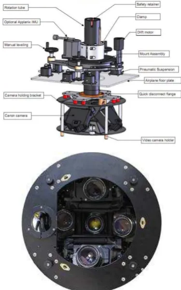
Sanborn acquired one MIDAS from TrackAir, in 2011. This system consists of four tilted (45 degrees) cameras and one vertical camera connected to a dedicated data acquisition computer system. The 5 digital cameras are based on the Canon EOS 1DS Mark3 with Zeiss lenses (Figure 1). The CCD size is 5,616 by 3,744 with the pixel size of 6.4 microns. The 5 cameras are installed in a special platform which fits in standard 22 inch or larger camera holes. Flight management and the 5 cameras are controlled in real time using TracKAir’s XTRACK FMS. In post mission, a suite of post processing software packages for flight planning, GPS/Inertial data processing, direct image georeferencing, and calibration and quality control are used to produce a set of five directly georeferenced images at each camera location. Each image is individually time-tagged using

individual timing devices for each camera of a microsecond absolute accuracy.

Multiple flights using different camera configurations (nadir/oblique (28mm/50mm) and (50mm/50mm)) were flown over downtown Colorado Springs, Colorado. Boresight fights for 28mm nadir camera were flown at 600m and 1,200m and for 50mm nadir camera at 750m and 1500m. Cameras were calibrated by using a 3D cage and multiple convergent images utilizing Australis model. Applanix CalQC software was used for boresight calibration, and Intergraph’s ISAT product was used for aerial triangulation. This paper provides some information about the MIDAS system specifications, boresight block layouts, experienced gained, issues encountered, and the accuracy obtained from the 28mm/50mm nadir and oblique blocks. Stability of the MIDAS system is also evaluated by analyzing several blocks flown at different GSDs.

more than 2 GSDs.

Cameras were calibrated by using a 3D cage and multiple convergent images utilizing Australia model. This model enables corrections for the camera distortions to a considerable extent, but leave very small systematic errors due to its own limitations. Correction grids were generated by analyzing the image residuals by collocation and self-calibration bundle adjustment was applied to model the remaining systematic errors. Intergraph’s ImageStation Automatic Triangulation (ISAT) software was used for tie point matching and bundle block adjustment. SimActive Correlator3D software was used to create DSM, DTM, and ortho mosaics. The results of the final bundle adjustments are sufficient to enable Sanborn to produce DEM/DTM and orthophotos from the nadir imagery and create 3D models using georeferenced oblique imagery. This paper does not discuss the DEM/DTM and orthophoto accuracy assessments.

Recommendations are provided for the future flights by eliminating the heat from the aircraft exhaust system and by capturing the images using the 50mm/50mm camera configuration and in RAW format.

Figure 1. MIDAS Camera Assembly

2. DATA PROCESSING

2.1 AGPS/IMU Processing

The airborne-GPS data were processed using POSPac (version 5.3) Mobile Mapping Suite; GPS-IMU tightly coupled processing software which uses Kalman Filtering techniques, and On-The-Fly (OTF) ambiguity resolution techniques. Multiple CORS stations are being used in

SmartBase trajectory processing.

2.2 SmartBase Processing

Applanix SmartBase processing mode creates a virtual base station, which follows plane trajectory allowing faster and more accurate on the flight kinematic ambiguity resolution. In order to process trajectory in SmartBase processing mode multiple CORS stations are imported into the project. The network of the CORS stations creates a closed polygon around the plane trajectory. Within the polygon atmospheric corrections are well modeled and applied to each photo center. The SmartBase quality check with respect to primary is performed on all CORS stations involved in the network. The final step in Applanix SmartBase processing is ‘GNSS -Inertial Processor’ which combines GPS CORS data with inertial data in tightly coupled process.

2.3 CalQC Adjustment

Applanix CalQC software is used to estimate the exterior orientation parameters, known as POSEO. 70 images from the 28mm block and four control points are used to compute the final POSEO data. In this process, CalQC generates image coordinates for each camera and from each altitude and estimates the IMU Misalignments, Datum Shift, and Camera Calibration parameters (optional) and arrives at the final POSEO data for the whole blocks.

The precise position of the camera lens node was interpolated from the trajectory of GPS positions utilizing polynomial fitting techniques. The time-tag for each event served as a basis for the interpolation.

The lever arm offset values are applied to this data resulting in a final AGPS file containing the coordinates of the camera lens node at each instant of exposure. Final Exterior Orientation parameters and positions are outputted using project assigned datum, projections and units.

CalQC Processing were performed in four steps to compute the MIDAS boresight and camera calibration parameters:

Step One:  Un-locked IO  No Datum Shift  Full control GCPs  Blunder Detection On

Step Two:

 Locked IO (adjusted values from step one)  Datum Shift

 Full control GCPs  Blunder Detection On

Step Three:

 Un-locked IO (adjusted values from step one)  No Datum Shift ((adjusted values from step two)  Full control GCPs

 Blunder Detection On

Step Four:

 Locked IO (adjusted values from step three)  No Datum Shift (adjusted values from step two)  Check GCPs (the RMS values indicate how POSEO

Step Four provided the final POSEO data and the camera interior orientation parameters (f, xp, xp (PPAC)).

2.4 Aerial Triangulation

The purpose of aerial triangulation is to densify horizontal and vertical control from relatively few ground control points (GCPs). Since obtaining GCPs is a relatively significant expense in any mapping project, AT procedures are used to reduce the amount of field survey required by extending control to all stereo-models.

This method is essentially a mathematical tool, capable of extending control to areas between ground survey points using several contiguous uncontrolled stereo-models. The surveyed control, along with the reduced image coordinates, and the exterior orientation parameters served as input into a combined block adjustment. Three–dimensional, simultaneous least squares adjustments by bundles, commonly referred to as “bundle” adjustments, were undertaken using PhotoT GPS adjustment software.

ISAT software is used for the Image matching and tie point generation and PhotoT module is used for the bundle block adjustment. Systematic errors, caused mainly by camera distortion, can be compensated by 3D cage (Laboratory) Calibration). The uncompensated camera systematic errors and errors due to the environmental conditions can be modeled by PhotoT’s in-situ camera calibration and/or “correction grid” options.

2.5 Camera Calibration

An accurate camera calibration method provides reliable values for focal length, principal point coordinates, lens distortion, and other camera systematic errors. Traditionally, cameras are calibrated in laboratories either by using goniometers and collimator banks or by using special test fields of various ranges in sophistication. These techniques enable corrections for the camera distortions to a considerable extent, but leave very small systematic errors due to their own limitations. Correction grids generated by analyzing the image residuals by collocation and self-calibration bundle adjustment are some techniques to model the remaining systematic errors.

Different calibration methods are used to model a camera’s lens distortion and to compute its interior orientation parameters (Madani, 1985):

 Laboratory Calibration (In-door calibration)

 In-situ System Calibration and Verification (Out-door calibration)

 Self-calibration

 Correction Grid by Collocation Adjustment (Madani, 2008a, 2008b)

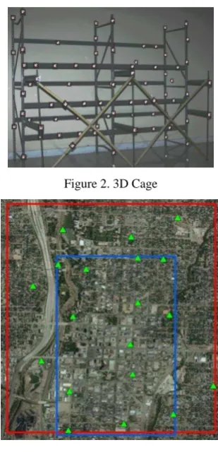
MIDAS systems were calibrated using a 3D cage and the Australis software (Figure 2). The Australis model, a sub-set of Brown model (Beyer, 1992, Fraser, 1997).

The dimensions of 3D cage were 120" x 151" x 74". About 78 retro reflector targets (16mm dots) and 30 images were used for the camera calibration. In this self-calibrating bundle adjustment, the object points and the camera exposure stations (XC, YC, ZC) were fixed, and the image point

coordinates (x, y) were weighted with the standard deviation

of 0.1 of a pixel. The unknowns were the camera’s rotation angles and the parameters of the Australis model.

The location of the principal point is not defined for most digital cameras and varies from camera to camera with the precision at which sensors are mounted into cameras and depends on the configuration of the frame grabber.

3. BORESIGHT FLIGHTS CONFIGURATION AND DATA ANALYSIS

 Dates of photography: October 2011  Average Terrain Elevation: 1820m

 Number of Control Points: 18 with accuracy of about 5cm in X, Y, and Z coordinate

 Horizontal Datum: NAD83, UTM, Zone 13  Reference Ellipsoid: GRS80

 Vertical Datum: NAVD88_Meters

Figure 2. 3D Cage

Figure 3- Boresight Flight Area, Downtown, Colorado Springs

156 images from the 28mm nadir low altitude flight and 36 images from the high altitude flight are used to estimate the highest possible accuracy for the MIDAS system (Figure 3).

Input Data:

 Camera calibration parameters (f, xp, yp, and lens distortion values)

 18 Control points with 5cm standard deviation  3 check points for accuracy assessment.

POSEO data with 5cm standard deviations for the exposure station coordinates (GPS) and 0.05 degrees for the attitude parameters (IMU).

Flight Name

Camera Config. (mm)

Flying Height (ft)

Number of strips

Number of Images

GSD (inch)

Boresight 28 / 50 2,000 14 386 5

Boresight 28 / 50 4,000 11 132 10.5

Garden of God

28 / 50 12 162 3.5 -

8 Air Force

Academy

28 / 50 6 102 4

Boresight 50 / 50 2,500 19 699 5

Boresight 50 / 50 4,500 19 318 7.5

Garden of God

50 / 50 6 114 3

Table 1. MIDAS Flight Configurations

3.1 Low Altitude Bundle Adjustment Results

Three different bundle adjustments were performed on the low and high altitudes 28mm nadir imagery (Table 1):

1. Bundle adjustment with constraining the GPS/IMU and some control points

2. Direct Georeferencing (fixing GPS/IMU data) and some control points

3. Refining POSEO data with check points

The bundle block adjustment results for the low altitude 28mm nadir block using GPS/IMU block shift are shown in the following tables (2-6).

Table 2. Bundle Adjustment + EO + Control

Table 3. Control/Check Points Residuals

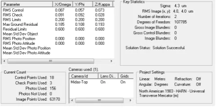
Estimated sigma (image measurement error) is 3.8um (0.6

pixel) and the RMS values for the control points and check points are 0.11m, 0.06m, 0.08m and 0.13m, 0.10m, 0.075m (about 1GSD (0.13m), respectively. The amount of the GPS block-shift in X, Y, and Z direction are 0.03m, 0.04m, and 0.04m, respectively.

Table 4. Direct Geo Referencing (DGR) + Control

The RMS values for the control and check points are less than 1 GSD (0.13m).

Table 5. Refine POSEO with Check Points

Table 6. Check Point Residuals

3.2 High-Altitude Block

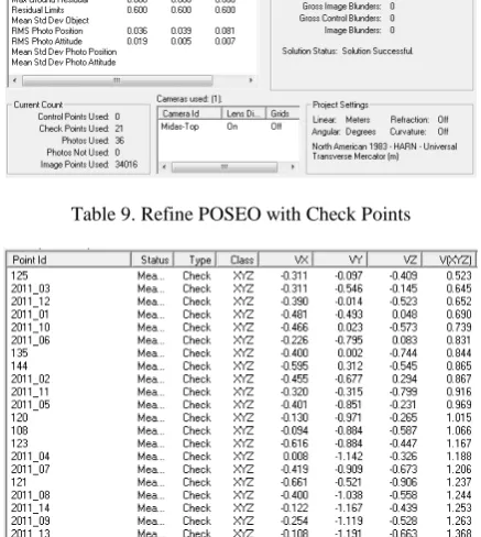
The same types of adjustments were also performed on the 36-image block of the 28mm high altitude flight. The RMS values of the check points are much smaller than the 27cm, the GSD of this flight.

The following tables (7 to 10) provide additional statistics about these adjustments.

RMS values of 21 check points are about one GSD (0.13m) for planimetry and 2 GSDs for vertical.

There is not any systematic pattern or large residuals in the camera positions. Again, this indicates that the data fits very well to the ground.

Table 7. Bundle Adjustment + EO + Control

Table 8. Direct Geo Referencing (DGR) + Control

Table 9. Refine POSEO with Check Points

Table 10. Control and Check Point Residuals

The RMS values of 21 check points are about 2 to 3 GSDs (27cm) for X, Y, and Z coordinates.

3.3 Bundle Adjustment Results of All Five Cameras

It is not necessary to perform the bundle adjustment for the oblique imagery as long as the boresight calibration (CalQC) provides the accurate exterior orientation for each block. In this study, image matching and bundle adjustment were also performed on all five cameras. ISAT was able to generate tie points for all oblique imagery. This capability allows us to refine the exterior orientation of the oblique imagery for a better and more accurate 3D model extraction.

Again, three different bundle adjustments were performed on all MIDAS 28mm boresight block (386 images for the low altitude flight and 132 for the high altitude flight) with 18 control points and 4 check points (total of 30 adjustments!). The overall RMS values of the check points in X, Y, and Z coordinates ranged 0.08-0.20, 0.05-0.15, 0.08-0.20 for the low altitude block and 0.1-0.3, 0.07-0.35, 0.08-0.45 for the high altitude block.

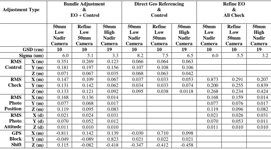
3.4 Bundle Adjustment Results of 50mm Boresight Blocks

The same bundle block adjustments were performed on the 50mm boresight (low and high altitudes). 17 control points and 4 check points were used in the 50mm boresight blocks. Again, three different bundle adjustments were performed on these blocks and the summary of the statistics are given in Table 11.

Principal point of auto collimation was adjusted and collocation grid was fitted to the observations of the 50mm low altitude block to remove the remaining systematic errors. The results of these adjustments are shown in column “Refine Low 50mmCamera”.

4. CONCLUSIONS AND GENERAL REMARKS

A modern professional digital oblique camera such as MIDAS is used to generate lifelike three dimensional to the users for visualizations, GIS applications, architectural modeling, city modeling, games, simulators, etc. Oblique imagery provide the best vantage for accessing and reviewing changes to the local government tax base, property valuation assessment , buying & selling of residential and commercial for better decisions in a more timely manner. Oblique imagery is also used for infrastructure monitoring making sure safe operations of transportations, utilities, and facilities.

Table 11. Bundle Adjustments Results of the 50mm Configuration Blocks

Strips were flown in one direction in both high and low altitudes, which makes IMU boresight and principal point of auto collimation (PPAC) indeterminable. But, due to two different GSDs (14cm and 27cm), it was possible to boresight these blocks. Due to issues with the CalQC software, it was only possible to use 70 images and 4 control points for the boresight calibration.

Oblique cameras 2 and 5 of the 28mm configurations were affected by the heat from the exhaust (hot air from the exhaust system, moves in a spiral way). Some odd color striping was found in random images. These artifacts only occurred in the oblique cameras and only occurred on colored rooftops. The uncorrected JPEG format caused some image blur. The decision to use JPEG instead of RAW is not easy, especially when a high trigger rate is required. This should not be an issue for 3D model applications since the image size will be reduced. Cycle rate is 2.5 to 2.7 seconds for raw format. It is possible to use smaller cycle rate (1.7 seconds) for smaller GSDs but the image format must be

JPEG. Low altitude flights make the aircraft unstable, the leveling of the MIDAS system might be extremely difficult, and the operator has to check very thoroughly for eventual cut offs based on the extreme leveling.

The biggest issue appears to be that the wider angle from the 50mm lens system causes obstruction from the plane in every image in camera 4 and the exhaust issues persist as seen previously. Rooftop striping also appears in this set of raw imagery. This imagery was also captured in Jpeg format.

5. REFERENCES

Beyer, H., 1992. Geometric and Radiometric Analysis of a CCD-Camera Based Photogrammetric Close-Range System,

Institut für Geodäsie und Photogrammetrie, an der Eidgenössische Technische Hochschule, Zürich, Dissertation ETH Nr. 9701.

Fraser, C., 1997. Digital camera self-calibration, JPRS, April, Vol. 52, No. 4, pp. 149-159.

Höhle, J., 2008. Photogrammetric Measurements in Oblique Aerial Images, Photogrammetrie Fernerkundung Geoinformation, 2008, issue 1, pp. 7-14

Jacobsen, K., 2008. Geometry of vertical and oblique image combinations

Madani M., 1985. Accuracy Potential of Non-Metric Cameras in Close-Range Photogrammetry Ph.D. Dissertation, Department of Geodetic Science and Surveying, Ohio State University

.

Madani, M., Shkolnikov, I., 2008a. International Calibration and Orientation Workshop, January 30th – February 1st, 2008, Castelldefels, Spain