isprsarchives XXXIX B1 267 2012

ITS IN-FLIGHT RADIOMETRIC AND GEOMETRIC CALIBRATION CONCEPT

M. Schneider1_{, R. Müller}1_{, H. Krawzcyk}2_{, M. Bachmann}1_{, T. Storch}1_{, V. Mogulsky}3_{, S. Hofer}3 1

Deutsches Zentrum für Luft- und Raumfahrt (DLR), Oberpfaffenhofen, Germany 2

Deutsches Zentrum für Luft- und Raumfahrt (DLR), Rutherfordstr. 2, 12489 Berlin, Germany 3

Kayser-Threde GmbH, Wolfratshauser Straße 48, 81379 Munich, Germany

Commission I, WG 4

KEY WORDS: Geometric Calibration, Radiometric Calibration, Hyper spectral, Satellite

ABSTRACT:

The German Aerospace Center DLR – namely the Earth Observation Center EOC and the German Space Operations Center GSOC – is responsible for the establishment of the ground segment of the future German hyperspectral satellite mission EnMAP (Environmental Mapping and Analysis Program). The Earth Observation Center has long lasting experiences with air- and spaceborne acquisition, processing, and analysis of hyperspectral image data. In the first part of this paper, an overview of the radiometric in-flight calibration concept including dark value measurements, deep space measurements, internal lamps measurements and sun measurements is presented. Complemented by pre-launch calibration and characterization these analyses will deliver a detailed and quantitative assessment of possible changes of spectral and radiometric characteristics of the hyperspectral instrument, e.g. due to degradation of single elements. A geometric accuracy of 100 m, which will be improved to 30 m with respect to a used reference image, if it exists, will be achieved by ground processing. Therfore, and for the required co-registration accuracy between SWIR and VNIR channels, additional to the radiometric calibration, also a geometric calibration is necessary. In the second part of this paper, the concept of the geometric calibration is presented in detail. The geometric processing of EnMAP scenes will be based on laboratory calibration results. During repeated passes over selected calibration areas images will be acquired. The update of geometric camera model parameters will be done by an adjustment using ground control points, which will be extracted by automatic image matching. In the adjustment, the improvements of the attitude angles (boresight angles), the improvements of the interior orientation (view vector) and the improvements of the position data are estimated. In this paper, the improvement of the boresight angles is presented in detail as an example. The other values and combinations follow the same rules. The geometric calibration will mainly be executed during the commissioning phase, later in the mission it is only executed if required, i.e. if the geometric accuracy of the produced images is close to or exceeds the requirements of 100 m or 30 m respectively, whereas the radiometric calibration will be executed periodically during the mission with a higher frequency during commissioning phase.

1. INTRODUCTION

The future German satellite mission EnMAP addresses hyperspectral remote sensing with the major objectives to measure, derive and analyze diagnostic parameters for the vital processes on earth’s land and water surfaces (Kaufmann et al., 2006; Kaufmann et al 2009; Müller et al., 2006; Rossner et al 2009; Stuffler et al 2007). Derived geochemical, biochemical and biophysical parameters serve as input for physically based ecosystem models and ultimately provide information reflecting the status and evolution of various terrestrial ecosystems. Applications comprise agriculture, coastal zones, land degradation, geology and forest themes.

The EnMAP satellite will be operated on a sun-synchronous orbit at 653 km altitude with a global revisit capability of 21 days under a quasi-nadir observation, namely with an across-track tilt of at most 5°. The satellites across-across-track tilt capability of up to 30° allows a revisit time of four days. The attitude and orbit control system (AOCS) payload will contain three star sensors, gyros and GPS. The hyperspectral imager (HSI) will consist of two pushbroom imaging spectrometers to cover a broad spectral range from 420 nm to 2450 nm: a 2-dimensional CMOS (Complementary Metal Oxide Semiconductor) detector array for VNIR (visible and near infrared) with approximately 96 spectral channels, i.e. 6.5 nm spectral resolution, and a 2-dimensional MCT (Mercury Cadmium Telluride) detector array

for SWIR (shortwave infrared) with approximately 136 spectral channels, i.e. 10 nm spectral resolution. The HSI is designed and realized by Kayser-Threde GmbH. The launch is planned for 2015. During the complete mission lifetime of five years, the spectral and radiometric behavior of the sensor varies within narrow limits. Therefore, in-flight calibration is necessary to ensure a spectral accuracy of better than 0.5 nm and radiometric accuracy of better than 5%. In this paper, an overview of this in-flight radiometric calibration is presented.

2. CALIBRATION APPROACH

The HSI will be subject to extensive characterization and calibration measurements in laboratory before launch. Thus, all necessary instrument characteristics are tabulated and for all measurements using internal sources corresponding pre-launch reference data are generated. After reaching the desired orbit, the first task is to perform the in-flight calibration to establish a link between pre-launch and post-launch characteristics. This comprises a check for changes in instrument characteristics during launch (expected due to air-vacuum transition and gravity release), to generate the initial post-launch calibration reference data, to establish the initial spectral and absolute radiometric calibration and to establish the geometric calibration. During commissioning phase, all calibration measurements will be performed with a high frequency, as the most significant changes of the instrument performance are expected shortly after the launch and during the first time in orbit.

3. RADIOMETRIC CALIBRATION

The design of the HSI provides a suite of technical tools (Mogulsky et al, 2009) and operational modes to perform the necessary measurements for on-orbit calibration and monitoring of instrument properties throughout the mission, in particular: Shutter/calibration mechanism for dark value and calibration measurements, full aperture diffuser for Sun calibration (radiometric, absolute), main integrating sphere (white Spectralon®) for relative radiometric assessment, secondary sphere (doped Spectralon®) for spectral calibration assessment and focal plane LEDs for linearity measurements. In this chapter, an overview of these measurements is given.

3.1 Dark Value Measurement

Each calibration and Earth observation measurement is accompanied by at least two series of dark value measurements to correct the dark current offset of the VNIR and SWIR detector output signal. The first series starts before the light measurement and the second afterwards. During pre-processing and analysis of the dark signal, the following steps are executed: check for outliers, dead/bad pixel flagging, averaging measurements with low/high gain (before/after), comparison to reference data and interpolation between before and after dark measurements. The dark values required to correct the calibration and Earth observation data are calculated during pre-processing as follows:

∑

=

=

n

i

dark k j i dark

k

j

DN

n

DN

1 , , ,

1

₍₁₎

where

dark k j

DN

, is the mean value of dark measurements for

row pixel j and spectral channel k,

DN

_idark_,j,k is the pixel value of a dark measurement for frame readout i, row pixel j and spectral channel k and n is the number of frame readouts of dark measurements. An additional step is performed for the SWIR detector. Unlike in the VNIR part of the spectrum, the shutter may cause a residual radiation in the SWIR, which leads to an error in the measured dark value. This effect can be corrected by using dark values obtained by deep space looking measurements since shutter temperature is expected to be highly constant. The signal caused by radiation from the shutter (DNshutter) is calculated as difference between the signal measured at closed

shutter and that measured at open shutter for deep space viewing. The dark values measured during sun calibration for closed shutter are corrected accordingly by subtracting DNshutter_. If DNdarkj,k (ds, ws) is the mean value of dark measurement in

deep space (ds) with shutter (ws) and DNdarkj,k (d, wos) the mean

value of dark measurement while looking the instrument in deep space without shutter (wos) then the mean value of current (c) (outside of deep space) shutter measurement in SWIR is:

[

( , ) ( , )

]

) ( 1

, ,

1 , ,

, DN c DN dsws DN ds wos

n

DN darkjk

dark k j n

i k j i dark

k

j =

∑

− −

=

(2)

3.2 Sun Calibration

A sun calibration sequence consists for both channels (SWIR, VNIR) of dark value measurements with both low and high gain, the sun measurement with low gain and high gain and the again dark value measurement with both low and high gain. After the dark value measurements have been processed as described in chapter 3.1, all necessary corrections (Non-Linearity, Straylight, Spectral Referencing and Geometric) will be applied and the averages for each row pixel in each spectral channel for both measurements at low and high gain setting are computed. Then, the results are compared to the previous measurement and corresponding valid Sun calibration reference file.

If the data keep within the given reference limits no action has to be taken with respect to radiometric calibration. The data are archived and used for further monitoring statistics. If the deviation exceeds more than half of the radiometric requirement, a detailed analysis is necessary to identify the reasons to confirm possible changes in instrument performance. If the changes are confirmed, new radiometric calibration factors are computed and the radiometric calibration table is updated. The calibration equation for the data is:

sun k j k j k

j

C

DN

L

_,

=

_,

⋅

, (3)

where

C

_j,kis the calibration coefficient of row pixel j and spectral channel k,

DN

sunj,k is the corrected mean sun value of

row pixel j and spectral channel k and

L

_j,k is the extraterrestrial radiance of row pixel j and channel k. During sun calibration of the HSI, the irradiance from the sun will be converted to radiance using the diffuser.

Using a reference table of extraterrestrial irradiance values of the sun in the wavelength region from 400 nm to 2500 nm and the conversion equation from irradiance to radiance (4), the calibration coefficients can be derived from Sun calibration as given in (5).

SE k j k

j k

j

E

BRDF

K

L

,

=

0, ,

⋅

,

⋅

(4)

sun k j SE k j k

j k

j

E

BRDF

K

DN

C

_,

=

(

_{0, ,}

⋅

_,

⋅

)

/

, (5)

where

E

0,_j,_kis the extraterrestrial irradiance of row pixel j and spectral channel k,

k j

BRDF

_, is the bi-directional reflectance function of row pixel j and spectral channel k and

K

_SE is the

3.3 Relative Radiometric Calibration

Relative radiometric measurements are performed in order to assess instrument stability. During a relative radiometric calibration sequence, the light from main sphere is measured on five different light levels, each framed by dark value measurements with both low and high gain. The focal planes are operated as in Earth observation mode, i.e. with automatic gain switching for the VNIR channel and preset gains for SWIR. The dark values are processed as already described in chapter 3.1. After dark signal correction the frame readouts are averaged for each illumination level and then compared to the corresponding reference values. If the difference of the current measurements and the reference values exceed a defined limit in the order of desired radiometric accuracy, a repeated measurement is proposed to confirm the result. A more detailed analysis of the measurement data (including housekeeping and health data) and comparison to other measurement data (e.g. secondary sphere, focal plane LEDs) should give confirmation and allow conclusions for the reason of deviations. In any case, if the change is confirmed, the reference data will be updated and a calibration update (Sun, spectral) might also be required.

3.4 Spectral Calibration

There are different possibilities to check and verify the spectral calibration of the instrument basically by the use of the secondary sphere with doped Spectralon® coating. The secondary sphere is the baseline for operational spectral check and calibration, the use of atmospheric features is currently a more experimental part of the scientific validation activities. However, since it potentially allows for higher precision it might become part of the operational procedure at a later stage. During a spectral calibration sequence, the light from secondary sphere is measured with dark value measurements with high and low gain both before and after the calibration. After the processing of the dark value measurements (chapter 3.1) and the necessary corrections, the readouts are averaged and compared to the reference values. If the difference of the current measurements and the reference values exceed a defined limit, a repeated measurement will be performed to confirm the result. A more detailed analysis of the measurements data (including housekeeping and health data) and comparison to other measurements (e.g. atmospheric absorption features) will give confirmation and allow conclusions for the reason of the deviations. In any case, if the change is confirmed, the reference data and spectral calibration table will be updated. In this case also an update of radiometric calibration is required.

The task of the spectral calibration is the determination of the adjustment of the pre-launch allocation of the focal detector pixels to their wavelengths. Every element of the sensor with coordinates (k, j) is assigned to a pre-launch central wavelength through laboratory analysis, whereas index j represents the spatial row pixel and coordinates k the spectral channel. HSI is designed such that wavelength λ(k, j) is constant for a fixed spectral coordinate k (k=const). The in-flight spectral calibration determines the deviation of the current centre wavelengths of each detector pixel from their pre-launch reference values with the use of the secondary sphere coated with doped Spectralon® _{with its characteristic selective spectral} reflectance. The adjustment is carried out under the assumption, that all changes are small and smooth. In the opposite case one has to suppose a fatal incident what needs additional investigations and special actions.

Initial point is the pre-launch laboratory calibration of the detector and the spectrally doped secondary sphere, giving the

reflectance R(λ) or the spectral radiance L(λ) of the sphere according to the illumination with the inner lamps, together with the corresponding λ(k,j) wavelength array. The wavelength correction will then be derived from the in-flight radiance measurements L(k,j) of the sphere. Due to the complexness of the complete task there are two methodologically different approaches proposed to ensure and enlarge the quality of the results. For the practical realization of the approaches both need more theoretical accuracy investigations.

3.4.1 First Approach

In a first approximation it is assumed that pre- and post-launch wavelengths are perpendicular to the spatial direction on the sensor, e.g. λ(k,j=const) = const. Then one can calculate a central wavelength for the kth

spectral channel averaging over all spatial row pixels, analogously for the measured radiances or reflectances. The inner lamps are powered up and the measured digital numbers are subjected to the standard radiation calibration procedure with dark signal, non-linearity and stray light correction giving the actual radiance array L(k,j), which then is also averaged over j. This spectrum will be compared to pre-launch values. To suppress noise, a number of measurements is repeated and averaged over time. The selective spectral reflectance dependence of the secondary sphere allows a selection of at least five strong local maxima in L(k) for each of the two spectral ranges, which can be used as basic points for inter-comparison. From both pre-launch and post-launch values, the corresponding local maxima are found. One can derive a regression between pre- and post launch positions of maxima (k,k’). The regression can be easily made linear or quadratic (even other dependencies) and then used to derive the new wavelength assignment

))

(

(

=

)

(

=

)

(

'

'

post

k

λ

pre

k

λ

pre

k

k

λ

(6)

giving now the actualized post-launch wavelength accordance to spectral pixel numbers k’ on the sensor.

This concept uses only a limited number of spectral base points with some local maxima for the investigation and is planned to be expanded to the entire spectrum in a way that brings both pre- and post-launch radiance spectra L(k) and L∗(k’) into maximal accordance to account for the spectral smile effects.

3.4.2 Second Approach

The second approach is a spectrum-matching technique. The first step is pre-processing of the dark signals and spectral measurements including corrections for dark current, non-linearity and stray light. The resulting matrix DNspectralonj,kwhich

contains the corrected set of digital numbers of the Spectralon® plate measurement for each detector element (j,k), where j indicates the spatial row pixel and k the spectral channel dimension.

The second step is radiometric calibration, i.e. conversion of the DNspectralonj,k values to radiance values Lspectralonj,k for each

detector element. The same algorithm will be applied as for radiometric calibration of image data.

Third step is matching of simulated radiances Lj,k to the

measured values Lspectralonj,k in order to obtain the center

wavelength λ(j,k) of each detector element. Matching is based on the assumption that the center wavelengths of the actually valid spectral calibration table λ0

∫

∫

+

+ ⋅

+ ⋅ + =

λ δ λ

λ δ λ δ

λ δ

λ δ

d r

d R

L r

L

j j k

j spectralon j

lamp j j k j j k

) (

) ( )

( ) ( ) (

, ,

,

(7)

where the following functions are known from pre-launch characterization: rk,j(λ) is the spectral response function (SRF)

of spectral channel k and row pixel j, Llamp(λ) is the spectral radiance of halogen lamps illuminating the secondary sphere and Rspectralon(λ) is the spectral reflectance of coating of secondary sphere (doped Spectralon®_).

The matching is then performed by calculating the residuum for different wavelength errors δj as follows:

∑

=

−

=

Channels

k

j j k spectralon

j k j

j

L

L

1

2 ,

,

(

)]

[

)

(

Res

δ

δ

(8)

Since a deviation from initial calibration of more than ±5 nm is very unlikely, and since spectral calibration accuracy should be 0.5 nm in the VNIR and 1 nm the SWIR, δj will be iterated from -5 nm to +5 nm in steps of 0.2 nm. The spectral error δj of row pixel j corresponds to the δj with minimal residuum.

This procedure can be performed, in principle, for all 1000 valid spatial pixels. However, it is very unlikely that δj will

differ from one spatial pixel to the next; if there is a pixel dependency at all, it will be probably a smooth function with few parameters. Furthermore, the uncertainty of δj depends on

sensor noise and remaining pixel-dependencies of the function rk,j(λ). This uncertainty can be reduced by averaging the spectra

of adjacent pixels. Since the change of the instrument's spectral properties between laboratory and flight can be determined only after launch, the procedure will be optimized during the commissioning phase. Optimization will determine the pixel dependency of δj, the number and location of row pixels, which

will be taken to determine δj, and the number of adjacent pixels

to be averaged.

Fourth step is the calculation of a new spectral calibration table λ(j,k). This will be done only if any δj is above the threshold

value of 0.2 nm by adding the resulting δj to the old center

wavelength. Note that here a pixel dependent shift is explicitly accounted for, corresponding to a change of the smile effect. The SRF is assumed to remain the same in orbit as on ground; it cannot be determined in-flight.

3.5 Linearity Measurements

The current baseline is to use look-up-tables for nonlinearity correction. Whether a polynomial or analog parametric fit correction is useful needs to be investigated and fixed during pre-launch characterization. Since the illumination is kept constant during the measurement the read signals in digital numbers (DN) are expected to be proportional to the integration time. Due to non-linearities in the detector itself or in signal handling electronics it will happen, that the real read value for integration time k DNk* is off the linear curve (may be below or

above). In this case the readout value will be replaced by the correct value DNk from the look-up table (LUT). This principle

is also applied to the linearity correction measurement: as long as non-linearity does not change, the corrected values for all integration times will correspond to the LUT values. In the case of deviations the LUT must be updated by replacing the DNk*

with the ones from the current measurement.

3.6 Spectral overlap of VNIR and SWIR instruments

At the spectral edges of the two VNIR and SWIR instruments there is an overlap of 12 channels with nearly identical spectral properties, i.e. central wavelength and bandwidth. This region will be additionally used to monitor the absolute and spectral calibration properties. With nominal instrument behavior the differences of the measured scene values shall not exceed the expected radiometric accuracy limits of about 5%. The definition of the absolute calibration coefficients bases on the illumination of both devices with an identical source (sun) and using the same diffuser. Due to small spectral deviations and separate internal noise processes small deviations are expected and accepted.

4. GEOMETRIC CALIBRATION

Geometric processing of EnMAP scenes will be based on laboratory calibration results. This comprises instrument/star-sensors alignment (instrument boresight) and pixel boresight (look angles/line-of-sight vectors of individual pixels), where both types of measurement are given for a range of temperatures to be expected under on-orbit conditions.

During repeated passes over selected calibration areas images that are distributed over a large latitude range, will be acquired. The update of geometric camera model parameters will be done by an adjustment using ground control points, which will be extracted by automatic image matching (Lehner and Gill, 1992, Schneider et al., 2011). In the adjustment, the improvement of attitude angles (boresight angles), the improvement of interior orientation parameters (view vector) and the improvement of position data will be estimated. As these values are correlated, a weighting is needed. Therefore, the a priori variances of the measured values are introduced in the adjustment. The initial parameters of the sensor model are derived from laboratory calibration (respectively, from currently valid geometric calibration tables).

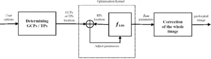
Figure 1 shows from the graphical point of view the concept of georeferencing by inversion of the LOS model.

Figure 1: Georeferencing concept by inversion of the LOS model.

4.1 Calibration Coefficients

In this chapter, the parameters that are calibrated are described, giving also an insight of the geometric processing.

4.1.1 Interior Orientation

x

ψ

and

ψ

_yas illustrated in figure 2. The angles are in decimal degree.

Figure 2: Definition of object sided pixel view directions

The pixel view vector is then calculated by

 polynomial. The initial polynomial coefficients are derived from pre-launch geometric calibration (about 20 support points) with an accuracy of better than 1.0 arcsec. The keystone is described by wavelength depended coefficients accounting for possible keystone effects.

2

g are polynomials with

{

( ), ( ), ( )

}

)

(λ x λ x λ x λ

x a b c

g ∈ , gy(λ)∈

{

ay(λ),by(λ),cy(λ)

}

.

The central wavelength

λ

is tabulated w.r.t. the channel number in the metadata (central wavelength values are determined at pixel index i = 500). The polynomial coefficients are estimated during calibration. Currently, the keystone effect is not accounted for and therefore, the wavelength dependent coefficients are set to zero.

4.1.2 Instrument Mounting Angles

The boresight alignment angles describe the relation between the coordinate frames of the payload instruments – namely the body (STS) and the sensor (HSI) coordinate frame. They are determined in a first step by pre-launch laboratory calibration. Due to e.g. gravity release effects these values are refined in a second step by in-flight calibration during the commissioning phase. In order to account for rotational variations of the instrument mounting angles during satellite orbit cycles – which are mainly affected by thermal influences due to the sun exposure time of the satellite – an additional rotational matrix in small angle approximation is introduced.

( )init y( )init x( )init

angles to rotate the HSI coordinate frame into the STS coordinate frame around the x, y, z axes, respectively. The variation of the instrument mounting angles is described by polynomial functions. The coefficients n_x0...10,

n

_y0...10and

10 ... 0

z

n are set to zero initially and modeled if a noticeable variation is detected.

10

where the normalized time period

T t

s= acc (tacc: accumulated

time the satellite is exposed to the sun before a scene is acquired; T: orbit period of 98.7 minutes) accounts for the time that satellite is exposed to the sun before image acquisition.

4.2 Boresight Angles

In this chapter, an example for the improvement of the boresight angles is provided. Other values and combinations follow the same rules.

Rewriting the collinearity equation which relates the coordinates of an object point m

Object

r

expressed in any Earth bound mapping coordinate frame (index m used for a unique mapping coordinate frame) to image coordinates

r

_ObjectSensor:

r

R

R

r

r

ObjectSensor

body

where Sensor object

r

is the pixel view vector described in the sensor coordinate frame,the transformation

R

m_bodydenotes the rotation around the angles ψ=(ω,ϕ,κ) from the body to a mapping coordinate frame, which is derived from the angular measurements by the on-board attitude system, s is a scale

factor and

r

_Sensorm is the position of the sensor projection centre. The unknown boresight misalignment matrix is given by:

)

These Euler angles of the boresight misalignment matrix are determined by least squares adjustment using the inverse formulation of the LOS model. After rearranging the collinearity equation, the sensor coordinates can be expressed as

 divided by the equation for the z-image co-ordinate, which is the constant focal length f. The scale factor s cancels out.

In this equations the functions for Sensor Object

x and Sensor Object

y depend on the three unknown angles

{

}

point (GCP) is given by the measured image coordinates

sensor GCP sensor GCP y

x , and the corresponding object space coordinates m

GCP

r which are inserted into the equations. To this end the non-linear functions are non-linearized with respect to the three unknowns

ε

=

{

ε

₁

,

ε

₂

,

ε

₃

}

by Taylor expansion and evaluated at the interpolated exterior orientation parameters at the GCP, which leads to the system of linear equations

x A

p = ⋅

  

 

  

 

       

 

       

 

∂ ∂ ∂ ∂ ∂ ∂

∂ ∂ ∂ ∂ ∂ ∂

=

    

 

    

 

− − =

z y x

i

GCP z Sensor Object i

GCP y Sensor Object i

GCP x Sensor Object

i

GCP z Sensor Object i

GCP y Sensor Object i

GCP x Sensor Object

i

GCP Sensor Object i Sensor Object

i

GCP Sensor Object i Sensor Object

d d d

y y

y

x x

x

y y

x x

ε ε ε

ε ε

ε

ε ε

ε

 



 (17)

This system of linear equations has to be solved iteratively.

(

A A

)

A p

x₌ T −1 T ₍₁₈₎

with known values for the boresight angles (tilt mirror, stereo angle,…) as initial values of the iterative least squares adjustment. It is noted that a strong correlation can exist between parameters of the LOS model and not all parameters can be estimated (in the sense of physical values) simultaneously, especially for single imagery. For the estimation of sets of parameters a weight matrix W, which accounts for the different accuracies of the observation groups, is part of the adjustment process:

(

A A

)

A p

x= TW −1 TW ₍₁₉₎

Thermal influences will be modeled by a latitude model, where the parameters are given subject to the sun exposure time of the satellite, i.e. a polynomial of degree 2 for the boresight angles. The output calibration tables will consist of two matrices for the boresight angles and the parameters for a function modeling the interior orientation. In the first matrix, a fix offset of the boresight angles will be given, while in the second matrix, the additional boresight angles will be given subject to the sun exposure time of the satellite. Additionally, the improvement of the position data will be given as offset and drift.

Test sites are normally represented by accurate orthoimages with appropriate resolution (10 m to 30 m). The selection of calibration areas should account for the stability of the land use patterns and a global distribution, especially in latitude.

5. CONCLUSIONS

Additionally to extensive calibration measurements in laboratory, in-flight calibration is necessary to assess radiometric, spectrometric and geometric characteristics of the German hyperspectral satellite mission EnMAP hyperspectral instruments in orbit. A detailed overview of the in-flight calibration of the EnMAP is presented, both radiometric and geometric.

6. ACKNOWLEDGEMENTS

The authors commemorate their late colleague Dr. Andreas Neumann, who has made a significant contribution to the calibration activities of the EnMAP mission.

Supported by the German Space Administration DLR with funds of the German Federal Ministry of Economic Affairs and

Technology on the basis of a decision by the German Bundestag (50 EE 0850).

7. REFERENCES

Kaufmann, H.; Segl, K.; Chabrillat, S.; Hofer, S.; Stuffler, T.; Müller, A.; Richter, R.; Schreier, G.; Haydn, R.; Bach, H. (2006): A Hyperspectral Sensor for Environmental Mapping and Analysis. In: IGARSS Space Hyperspectral Sensors, Denver, CO, USA.

Kaufmann, H.; Segl, K.; Guanter, L.; Chabrillat, S.; Hofer, S.; Bach, H.; Hostert, P.; Müller, A.; Chlebek, C. (2009): Review of EnMAP Scientific Potential and Preparation Phase. In: EARSeL SIG-IS Workshop; Tel Aviv, Israel.

Lehner, M. and Gill, R. S. (1992): Semi-automatic derivation of digital elevation models from stereoscopic 3-line scanner data, In: IAPRS 29 (Part B4), Washington, DC, USA

de Miguel, A., Bachmann, M., Makasy, C., Müller, R., Neumann, A., Palubinskas, G., Richter, R., Schneider, M., Storch, T., Walzel, T., Wang, X., Heege, T. and Kiselev, V. (2010) Processing and Calibration Activities of the Future Hyperspectral Satellite Mission EnMAP. In: Canadian Geomatics Conference 2010 - Technical Programme on CD-ROM, ISPRS Commission I, 15 - 18 June 2010, Calgary, Kanada.

Mogulsky, V.; Hofer, S.; Sang, B.; Schubert, J.; Stuffler, T.; Müller, A.; Chlebek, C.; Kaufmann, H. (2009): EnMAP Hyperspectral Imaging Sensor On-Board Calibration Approach. In: EARSeL SIG-IS Workshop; Tel Aviv, Israel.

Müller, A.; Kaufmann, H.; Hofer, S.; Chlebek, C.; Richter, R.; Gredel, J.; Segl, K.; Förster, K.-P. (2006): Instrument Requirements, Data Processing, and Mission Scenarios for the German Hyperspectral mission EnMAP (Environmental Mapping and Analysis Program). In: ARSPC Keynote, Canberra, Australia.

Rossner, G.; Schaadt, P.; Chlebek, C.; von Bargen, A. (2009): EnMAP – Germany’s Hyperspectral Earth Observation Mission: Outline and Objectives of the EnMAP Mission. In: EARSeL SIG-IS Workshop; Tel Aviv, Israel.

Schneider, M., Suri, S., Lehner, M. and Reinartz, P. (2011): Matching of high-resolution optical data to a shaded DEM. International Journal of Image and Data Fusion..

Storch, T., de Miguel, A., Müller, R., Müller, A., Neumann A., Walzel, T., Bachmann, M., Palubinskas, P., Lehner, M., Richter, R., Borg, E., Fichtelmann, B., Heege, T., Schroeder, M. and Reinartz, P. (2008): "The future spaceborne hyperspectral imager EnMAP: Its calibration, validation, and processing chain", Proc. 21st Congr. Int. Soc. Photogramm. Remote Sens., p. 1265.