STEREO RECONSTRUCTION OF ATMOSPHERIC CLOUD SURFACES FROM
FISH-EYE CAMERA IMAGES
G. Katai-Urban a,* V. Otte b, N. Kees b, Z. Megyesi a, P. S. Bixel b
a Kecskemet College, Faculty of Mechanical Engineering and Automation, Kecskemet, Hungary - (katai-urban.gabor, megyesi.zoltan)@gamf.kefo.hu
b TMEIC Corporation, Roanoke, USA - [email protected], [email protected]
Commission III, WG III/1
KEY WORDS: Fish-Eye Camera, Stereo Reconstruction, Spherical Camera Model, Nephology, Atmospheric Cloud Reconstruction, Dense Matching
ABSTRACT:
In this article a method for reconstructing atmospheric cloud surfaces using a stereo camera system is presented. The proposed camera system utilizes fish-eye lenses in a flexible wide baseline camera setup. The entire workflow from the camera calibration to the creation of the 3D point set is discussed, but the focus is mainly on cloud segmentation and on the image processing steps of stereo reconstruction. Speed requirements, geometric limitations, and possible extensions of the presented method are also covered. After evaluating the proposed method on artificial cloud images, this paper concludes with results and discussion of possible applications for such systems.
1. INTRODUCTION
1.1 Motivation
The reconstruction of objects visible on the open sky is an attractive topic for both practical applications related to aerial navigation or detection, and applied scientific fields of meteorology, astronomy, even photogrammetry. While the hardware setups that perform the measurement and provide data for such applications are changing from range scanners to active light measurement devices, the use of relatively simple, passive camera systems still hold some benefit as well as challenges. Over the last three decades many kinds of sky imagers have been
developed. In the 1980’s the main goal was to detect the whole
sky cloud coverage. The first whole sky digital imager was developed in 1984 (Johnson, 1989). This device captured digital images at blue and red wavelengths using a charge injection device (CID). By processing this data, the first automated cloud detection algorithm was developed which could identify each individual pixel as opaque cloud, thin cloud or no cloud. Following the daylight sensors development was begun in the
early 90’s on devices which could compute the coverage day and
night. Most of the devices were applied fish-eye lens with 180° field of view. The detectors have changed over the time: from CID devices, to grayscale CCDs, to RGB CCD sensors (Shields, 2013).
1.2 Cloud Detection History
Detecting clouds on sky images is a challenging task. The general cloud cannot be described by its shape, contour or structure. Color is the most informative property in segmentation of clouds in the sky.
Many different types of color based segmentation method can be found in the literature. The main difference between the techniques is their respective color model. The first approaches used special types of cameras which could detect light at specific wavelengths (Johnson, 1989). These wavelengths were near the blue and red colors. After the common CCD sensors become widespread the standard RGB color space was applied. The ratio
(R/B) or difference (R-B) of the red and blue channels was used
in the early 2000’s (Long, 2006; Calbó, 2008). In 2014 a systematic analysis was published (Dev, 2014) to determine which color channels are the best for segmenting clouds. This study includes other color models: HSV, YIQ, CIE. The results point out that the S channel of the HSV color model is one of the most promising channels for cloud segmentation. A proposal for a new candidate of color features, used for cloud segmentation, is discussed in the cloud segmentation chapter.
1.3 Stereo Reconstruction
The use of stereo or multi-view reconstruction of outdoor scenes has been well studied in past decades. These advancements combined with the development of cameras optics, sensors and continuously growing processing power contributed to the realization of many practical applications. Many applications target the reconstruction of surfaces (Salman, 2010) often from wide baseline images (Megyesi, 2006). The use of spherical stereo (Kim, 2013) has also been introduced to utilize the fish-eye lens cameras. However, the application of such passive stereo methods to reconstruct atmospheric cloud surfaces has not been addressed before.
1.4 Contents of the Article
This article presents a camera system and a method to reconstruct atmospheric clouds. Section 2 discusses the details of the camera setup. Section 3 summarizes 3D reconstruction, discusses specialties of cloud surface reconstruction from stereo fish-eye cameras, and presents details for the proposed reconstruction algorithm:
1. Cloud segmentation 2. Dense matching
3. Post correspondence filtering 4. Gap filling
Section 4 focuses on the special problem of segmenting atmospheric clouds as a necessary step for the reconstruction algorithm. An analysis of the geometric limitations of the The International Archives of the Photogrammetry, Remote Sensing and Spatial Information Sciences, Volume XLI-B3, 2016
proposed system and discussion on scalability is in section 5. Results are presented in section 7 and conclusions are drawn in section 8.
2. CAMERA SETUP
To capture clouds on the whole sky a special type of imaging system is required. The most efficient solution is to apply wide
field of view (FOV) cameras that are able to observe the sky 360° horizontally and 180° vertically. These omnidirectional optical
systems can be divided into two types: dioptric and catadioptric systems. Catadioptric systems consist of mirrors and lenses and are usually equipped with a downward-looking camera. These systems have a blind spot (behind the camera) and thus are not ideal for observing the whole sky. Dioptric systems, on the other hand, use an upward-looking camera equipped with a fish-eye lens that provide a large FOV without a blind spot but often have lower resolution on the sides of the image.
2.1 Geometry
To use a camera system for reconstruction purposes, a model is needed to determine what describes the projection of the camera world points to image points. The Pinhole camera is the most simple and most commonly used model in computer vision. The model contains a camera center and an image plane (see Figure 1-a). The scene points are mapped to the image plane by a line crossing the camera center. Since this model presumes that scene points are in front of the image plane, it cannot handle the special cases emerging with wide FOV. If the FOV is wider than 180° then the scene points could be on both sides of the projection line so the pinhole model is clearly not applicable.
(a) (b)
Figure 1. (a) Pinhole camera model. (b) Spherical camera model
On the other hand, the spherical projection model (Li, 2008) (see Figure 1-b) defines the unit sphere as the image coordinates which are mapped to a plane and can account for a 180°+ FOV. The scene point � is projected to a point P on the image sphere by normalizing the projection vector pointing from the projection center ( ) to the scene point. The unit vector = [��], can be projected to image point � using the following formula:
� = [��] = [� � ] [��] (1) where � is the distance from the optical center on the image and
� � is the focal length given as a function of �.
According to projective geometry (Hartley, 2003) a single camera is only enough to identify the ray coming from the reconstructed object. To reconstruct the 3D position of the
objects multiple cameras are needed. The object positions can be identified through triangulation discussed in section 3.1.
2.2 Proposed Setup
The distance between the cameras (baseline distance) should be determined during the camera system planning. The baseline distance has an effect on both the precision of the triangulation and on the ambiguity of the atmospheric cloud matching (see section 3.3). Maximum triangulation precision can be achieved if the angle of the projection rays is near perpendicular. Assume that the clouds are in the 1000-5000 m height range the baseline of the cameras should be 2000-10000 m. However, such distances are impractical both technically, and from the image processing perspective. Images taken with this baseline distance show too much geometric and photometric distortion, which makes the matching of cloud pixels unfeasible. In order to create a practical setup, a compromise baseline distance should be found to fit both criteria.
Two Canon T3i cameras are used with Sunex SuperFisheye™
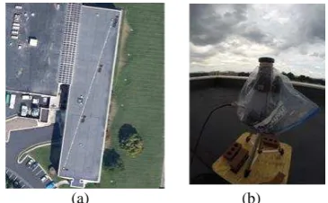
lenses to capture images. The cameras are installed on the top of a three story building to ensure the obstruction-free viewpoints (see Figure 2). Stands are applied to fix the cameras in face up position to the sky and are spaced 90 m apart. Synchronous capturing is essential in the case of moving objects so the camera system was synchronized with a common shooting signal. Images were taken in every 15 seconds.
(a) (b)
Figure 2. (a) Camera positions on the top of a three story building. (b) Camera installation on the roof
2.3 Calibration
The main goal during the camera calibration process is to estimate the parameters of the projection model. The spherical model; which can be described by Equation 1, the center of the unit sphere and focal length � � , these parameters still need to be determined. Through analysis of pictures from a known object, which has markers on different angles, these parameters can be estimated.
A calibration bowl, which is painted with concentric circles of uniform thickness, was posed in front of the camera (see Figure 3). By detecting the circles on an image and calculating the radius from the projection center the intrinsic parameters of the camera can be estimated.
The extrinsic parameters describe the position and orientation of
the cameras. The 185° field of view makes it possible to see the other camera on the image. Using this fact, the orientations of the cameras can be estimated. In the current experiment, the distance of the cameras were measured with GPS. These estimated extrinsic parameters are refined manually using known marker positions.
(a) (b) Figure 3. Calibration bowl
2.4 Rectification
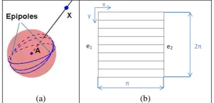
The goal of the rectification process is to transform the images using the intrinsic and extrinsic calibration data not just to fit perfectly to the spherical camera model but also to align the horizontal axis of the images with the baseline. After such image transformation the reconstruction can simply utilize the epipolar constraint i.e. each raster line of the stereo image pair will fall in the same plane (see Figure 4).
(a) (b)
Figure 4. Mapping the spherical image to the rectified image
The rectified images look as if the images were taken from cameras which were facing in exactly the same direction. According to the epipolar constraint, the projections of objects are found on the same horizontal line in each of the images (see (Salman, 2010) for details). This property can be exploited during the matching step of the reconstruction. Figure 13 shows an example of rectification.
In the case of the spherical model, the spherical image can be mapped directly to a rectified image. The epipolar curves on the sphere are transformed into parallel lines (as can be seen on Figure 4). The x Axis of the rectified image represents θ from 0
to π and the y Axis represents α from 0 to 2π (Li, 2008).
3. 3D RECONSTRUCTION
The goal of 3D reconstruction is to calculate the 3D coordinates of real 3D points that are visible on multiple images. To understand the reconstruction of multiple points let us first discuss triangulation, the technique used to calculate the 3D coordinate of a single point.
3.1 Triangulation
Consider Figure 5. Let P be a real world image, and let Pl and Pr
be P’s detected projections on the rectified images of the left and
right cameras respectively. Note that P lies on the intersection of lines connecting Cl with Pl and Cr with Pr. To calculate the 3D position of P the intersection of these lines must be calculated.
Figure 5. Triangulation
It must be noted that if the camera calibration is erroneous, then the position of P will also be misplaced due to the wrong real world position of Cl and Cr. Also, if the rectification is not perfect and the captured images do not match the spherical model, then Cl, Pl, Cr Pr will not be coplanar, therefore the Cl-Pl and Cr-Pr lines will be skew. In these situations the 3D point that minimize the summed distance to the two lines can be used instead of the intersection. In practice SVD can be used to find the closest point by employing the least squares method. More information can be found about triangulation in (Sonka, 2008; Hartley, 2003). To provide input to triangulation, it is clear that the accurate position of Cl and Cr must be known as well as the identities of the Pl and Pr projections of P. Depending on the number of reconstructed points, like P, determines whether Sparse or Dense Reconstruction should be used. Locating corresponding image points (like Pl and Pr) on the rectified images is a matching problem, and shall be discussed next.
3.2Sparse Matching
In sparse matching, selected image points with distinguishable properties are identified and corresponding points on the other images are found knowing that correspondences should have similar properties. The properties used to match in this case can be one or more feature descriptors like SIFT (Lowe, 2014), SURF (Bay, 2006) or MSER (Matas, 2002) just to list a few. These feature detectors propose candidate points and provide a reliable and distortion tolerant description that can be matched even in the wide baseline setup. To summarize, sparse matching provides a limited number of reliable points that can be used to reconstruct larger object structures, provide seed points for more dense approaches, and to verify or even auto correct calibration. Nevertheless, sparse matching is not suitable to reconstruct surfaces or dense volumes. For these purposes, dense matching is applied.
3.3Dense Matching
In dense matching the goal is to identify the projection of as many 3D points as reliably possible. The problem is that many of the target 3D points may be occluded, ambiguously distorted or have uninformative neighborhood; but a point set dense enough to reconstruct surfaces and large volumes still needs to be identified. Proposed solutions to overcome these problems include distortion invariant template matching (Megyesi, 2006; Mindru, 2004) and enforcing local neighborhood constraints in the energy function when searching for the most probable pixel positions. Often energy minimization frameworks or region growing methods are applied to limit the search and to handle homogenous areas.
Dense matching is a time consuming task, but many methods can be sped up by course to fine approaches (e.g. pyramid based The International Archives of the Photogrammetry, Remote Sensing and Spatial Information Sciences, Volume XLI-B3, 2016
processing), using a priori information from sparse matching, or performing feature based segmentation to limit the set of reconstructed points.
3.4 Dense Matching of Cloud Pixels
In the previous section 3D reconstruction was discussed in general. This section proposes a 3D reconstruction solution that is suitable to match cloud pixels. This solution needs to analyze the visibility of the object, their texture, and any observable distortions.
Geometric distortion: This type of error often occurs on wide baseline camera images as a result of the large change of perspective. In general, a planar surface suffers a perspective distortion that can be locally approximated by an affine transformation. There are dense matching methods that compensate this transformation (Megyesi, 2006) but to do so usually have performance costs. It can be said that the distortion is usually larger when the object distance is comparable to the baseline and if the surface normal is not facing the cameras. Neither of these conditions are typical in the setup mentioned here (see Figure 6); therefore, neglecting the geometric distortion is not a major mistake.
Photometric distortion: This type of error occurs when the camera sensitivities are set differently or the reflected light is different from the two cameras. This is especially problematic for clouds near the sun. In this application prior sun position information was used to mask sun region and avoid photometric distortion problems.
Infinity, Occlusion, Homogeneity, Ambiguity: these problems are the typical bottle necks for all stereo algorithms, and are generally difficult to handle. Their presence in the current scenario must be evaluated.
Infinity: Outdoor scenes often contain background objects at infinity. In this case pixels belonging to the sky are impossible to match, so they must be excluded from the matching. This can be achieved by applying Cloud Segmentation (discussed in section 4).
Occlusion: Since the typical object distances are multiples of the baseline, it is rare that clouds of different elevations are missed due to occlusion. Also, the bottom cloud surfaces show only limited 3D properties so occlusions within the same surface are typically limited. However, some minor cloud areas can be occluded this way so occluded pixels need to be detected. The suggested method to filter out bad correlations due occlusion is the Left-Right consistency or Stable Matching post correlation filter (Sara, 2002).
Homogeneity: The borders of the clouds are generally well textured. Unfortunately, the textured-ness of the cloud surfaces depends on the resolution level of our cameras. At higher resolution, the texture is less obvious, and can be ambiguous. This problem can be handled by Pyramid Matching. Matching is applied on the lowest resolution, then the results are refined on
each pyramid level. Also, segmenting the cloud using texture based segmentation has a positive effect on the matching. Ambiguity: Cloud regions that are well textured are unique in the majority of cases; therefore, this problem need not be handled
This step is crucial for handling problems of both Infinity and Homogeneity. This step is detailed in section 4. 2. Dense matching
Using Pyramid based template matching addresses Homogeneity and Ambiguity.
- Define a set of resolutions and the lowest resolution where information is visible.
- Perform template matching on the lowest resolution. - Propagate and refine matching results on higher resolutions.
3. Post correspondence filtering
To filter out false positives arising from Occlusion and Ambiguity apply a Left-Right consistency check: - Match from left image to right image.
- Match from right image to left image. - Keep consistent matches from the two results. 4. Gap filling
This step is often required if the cloud segmentation or the post correlation filtering produces missing pixels. Disparity information for the missing pixels can be filled from lower resolution matching of the Pyramid or by interpolating the neighboring consistent matches.
The result of this matching algorithm is illustrated in Figure 14 and 15. Figure 14 shows a disparity image which marks the displacement along the epipolar line with grey levels.
4. ATMOSPHERIC CLOUD SEGMENTATION
One crucial problem of reconstruction is how to prevent reconstruction of objects at infinity. In generic scenarios this requires the analysis of the matching results. In our application pixels at infinity are more easily separated because the majority of these pixels belong to the uncovered sky. These sky pixels can be separated prior to the reconstruction thus preventing matching on them. On a general sky image there are objects falling into five categories:
1. Sky pixels 2. Cloud pixels 3. Ground pixels
4. Sun (and Sun halo) pixels 5. Other airborne object pixels
In this application the intent is to reconstruct the cloud pixels; therefore, the rest must be detected and excluded.
Figure 6. Matching Clouds pixels: detailed view of a cloud region from stereo images
Ground pixels can vary in intensity and texture but separation is possible through applying geometric constraints (reconstructed ground objects can be ruled out by their elevation). Sun halo can be ruled out if the position of the sun is known; otherwise, these pixels are difficult to separate. Pixels belonging to the other airborne object category are difficult to separate because their texture, color, and intensity properties are unknown; and their position is indistinguishable from the clouds. Fortunately, the
other airborne object pixel’s size and rare appearance makes them statistically irrelevant. The problem that remains is the segmentation of the cloud pixels from sky pixels. Having evaluated several properties, it was found that the best separating feature is saturation. Examples can be seen in Table 1.
Table 1. Saturation Histograms from HSV and HSL color models
Sky image segments (Table 2) and cloud image segments (Table 3) are shown in the tables below with the registered values belong to the center pixel of the sample image. Histograms for specific features are shown in Table 1. These histograms can be used for automatic saturation based thresholding if the classes are distinctly separable. From the different saturation version the HSL Saturation values were found to be most effective; therefore, segmentation was based on this property. See Figure 14 as an
Table 2. Saturation values for non-cloud image regions
Cloud
Table 3. Saturation values for cloud image regions
5. GEOMETRIC LIMITATIONS
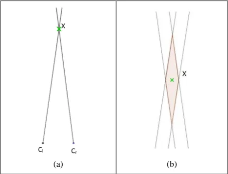
In the analogous case (presuming perfect camera calibration) the objects can be reconstructed at any distance with no error. In practice, the precision of the reconstruction highly depends on the resolution of the images and on how accurately the object pixels can be identified. See Figure 7-a, for illustration. Let � and �� be the camera centers of the right and left cameras, respectively, for a given baseline. The � scene point was triangulated using the intersection of the projection rays form the camera centers towards the point. Suppose the projected rays beyond the level of a pixel cannot be determined. � can then only be determined up the certainty defined by the bordering lines of those pixels thus forming a 3D quantization error hexahedron.
(a) (b)
Figure 7. Illustration of wide baseline
The 2D representation of this hexahedron is a quadrilateral (see Figure 7-b) resembling a parallelogram area. Inside this area � could be located anywhere. The worst case is when the real point is in the farthest corner but it is detected in the middle. The longest diagonal of the parallelogram shows the possible error range of the triangulated point. This error is minimal, when this hexahedron is close to a cube. In 2D this happens when ��� and
�� are perpendicular.
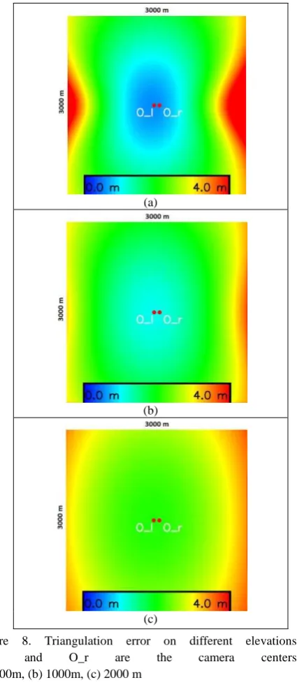
To analyze the behavior of the longest diagonal error indicator, the error values has been calculated for a set of points in a 3D cube around proposed camera setup. Using the proposed 90m baseline distance, the longest diagonals were calculated for each integer 3D position on a 3000x3000 m plane at different elevation levels. Sample results can be seen on Figure 8 (blue color represents lower error, red represents higher error).
Since for each 3D position, the accuracy is determined by the angle of the lines connecting the point the two camera centers, the space between the cameras at lower elevations has the best accuracy. Results are worse if the angle to the baseline is lower. Figure 8-a shows this effect. At lower elevation (500 m) and longer distances (1500 m) the angle to the baseline is small. In 0
these cases the parallelogram is very thin and the diagonal is long. If the elevation is increased (see Figure 8-b and Figure 8-c), the error becomes more uniform.
Using the proposed 90m baseline, the tests show that on the range of 1000-2000 m elevation (where the clouds will be detected) 90% of the area has maximum 4 m triangulation error. In this cloud reconstruction application these results are acceptable.
Figure 8. Triangulation error on different elevations. O_l, and O_r are the camera centers. (a) 500m, (b) 1000m, (c) 2000 m
Using geometric considerations it can be deduced that the baseline minimizing the geometric error is the double of the altitude of interest (e.g. 1000m for clouds at 500m). However, longer baseline will also generate perspective distortion typical on wide baseline images, preventing conventional stereo matching to work effectively. The practical trade-off between geometric accuracy and matching reliability will require yet lower baseline. The reliability of a reconstruction algorithm also depends heavily on the scene so if we constrain our
reconstruction to only clouds higher than 500m we arrive at a probable optimum baseline range between 500m & 1000m. To test one of these limits, we generated artificial cloud images using larger baseline, evaluated the results (see Section 6.) and came to the conclusion that using a 500m baseline the matching is still possible.
6. EVALUATION
We presented a camera setup and proposed a pipeline for reconstructing atmospheric cloud images, addressing the special problems of this application environment. The major features of this pipeline being Atmospheric Cloud Segmentation, Pyramid Matching, Consistency Filtering and Gap filling. To evaluate the combined efficiency of the pipeline we generated, two sets of input images with known scene geometry. One set of images was using synthetic Random Dot Stereo (RDS) images and another set was using a template of typical cloud images placed in a planar structure at different elevation levels. The first set is used to evaluate the reconstructed related steps without evaluating color segmentation, while the second set can be used to evaluate reconstruction efficiency of the whole pipeline.
6.1 Evaluation using Pyramidal Random Dot Stereo images
In general, the purpose of using RDS images is that it has unique information content around each pixel, allowing nearly perfect matching. RDS texture can be placed on any known scene structure providing ground-truth and allowing evaluation of reconstruction algorithm. However the RDS images need to be designed to match the application requirements. For the current application traditional RDS textures are ineffective as we apply matching on different scale levels. The information content on lower resolutions of the RDS is often lost. To use RDS for Pyramid Matching, we introduce Pyramidal Random Dot Stereo Images (PRDS). To generate these PRDS images we need to understand what the minimal physical size of a square is, which can be distinguished at different pyramid levels of the algorithm. With this knowledge, we can generate and upscale a low resolution RDS image, then randomly modify its pixel values. We can do this in multiple iterations to get a PRDS image. An example of that image can be seen in Figure 9.
(a) (b)
Figure 9. Pyramidal Random Dot Stereo Image (PRDS)
6.2 Evaluation results on Artificial Cloud images
To test the whole pipeline we also need to test the reconstruction combined with the Atmospheric Cloud Segmentation. For this, we generated artificial cloud images using a cloud template, which can be replicated on a planar structure. The period of the replication must be larger than the maximum disparity range on all levels. The planar structure can be positioned in different (a)
(b)
(c)
elevations to gain information on the accuracy of the algorithm w.r.t altitude or distance from the camera. A sample artificial cloud image can be seen in Figure 10.
(a) (b)
Figure 10. Artificial Cloud Image
(a) Cloud template, (b) Planar structure 6.3 Evaluation Results
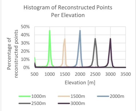
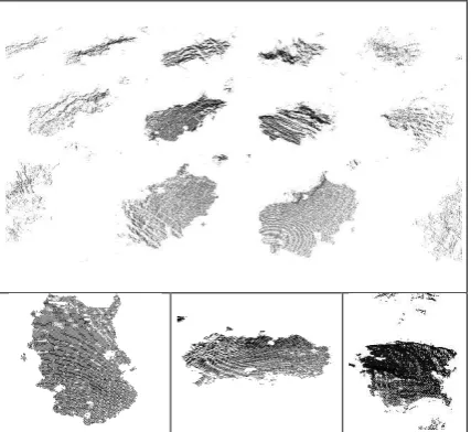
In our evaluation, we generated both PRDS and Artificial Cloud Images to test the reliability of the whole pipeline. The generated images replicated templates on a plane at different elevation levels, as if taken from cameras at increasing baseline. After running the reconstruction, histograms were created for the altitude of the reconstructed points. Since for each artificial point we know the correct elevation, any divergence from the ground-truth is the result of matching errors described in Section 3.3. A sample elevation histogram combining 5 different elevation levels can be seen in Figure 11. On this chart, we can see the percentage of the reconstructed points for each elevation, different colors indicate results for images on different elevation. We can see that the majority of the reconstructed points are within meters of the ground truth elevation, and only a small percentage of the reconstruction is erroneous. Based on these charts we concluded that the noise generated by the matching errors is acceptable. Visualized results of the reconstructed artificial point sets can be seen in Figure 15. The template cloud is recognizable as well as the repetitive structure of the input.
Figure 11. Histogram of the reconstructed points per elevation
7. RESULTS
This section reviews sample results generated from images acquired by our camera setup and using the proposed algorithm on those images. Starting from original images, the results are ordered as follows: rectification, segmentation, and reconstructed 3D points.
The proposed and installed stereo camera system captures images as seen on Figure 12. The fish-eye lens maps the sky to a round image.
After the calibration process, which was discussed in Section 2.3, the original images can be rectified (see Figure 13).
Before the reconstruction step the cloud pixels have to be segmented from the background. The threshold level of the saturation is set to include cloud colors and also sky parts which might be covered with thin cloud (see the result on Figure 14). For visualization of the 3D point cloud a disparity map is shown (epipolar displacement is converted to gray level) and a custom-made application rendering of each 3D point on top of the re-projected sky dome image.
8. CONCLUSIONS AND FUTURE WORK
A method to reconstruct clouds in 3D from two fish-eye lens cameras has been shown. The suggested method applies spherical camera model for rectification. After cloud segmentation, it uses dense stereo matching to generate point clouds. The matching and segmentation problems of cloud pixels was discussed and an algorithm that handles the problems relevant to this application was proposed. The effectiveness of the matching has been demonstrated on both artificial images with ground-truth and on real images. The reconstruction of 3000x3000 images run within 2 seconds on a Core i7 processor making it feasible to reconstruct clouds from image streams. Further optimization is possible. This cloud reconstruction method can be used to model and track clouds on the sky. This can be beneficial to many applications ranging from space research to meteorology. The cloud positions can also be used to calculate and track the cloud motion which also may have wide applications. Further improvements are possible by extending the stereo camera system to a multi view system.
ACKNOWLEDGEMENTS
This work was supported by TMEIC Inc.
Figure 12. Original Images
500 1000 1500 2000 2500 3000 3500
P
Figure 13. Rectified Images
Figure 14. Result of segmentation (left) and result of dense matching (right). Brighter pixels indicate larger disparities.
Figure 15. Visualization of the reconstructed artificial clouds
REFERENCES
Bay, H.; Tuytelaars, T.; Gool, L. V.; 2006. SURF: Speeded up robust features. Proceedings of the Ninth European Conference on Computer Vision, vol. 3951, pp. 404–417, 2006.
Calbó, J.; Sabburg, J.; 2008. Feature extraction from whole-sky ground-based images for cloud-type recognition; Journal of Atmospheric and Oceanic Technology, vol. 25, no. 1, pp. 3-14, 2008.
Dev, S.; Yee Hui Lee ; Winkler, S.; 2014. Systematic study of color spaces and components for the segmentation of sky/cloud images; Image Processing (ICIP), 2014 IEEE International Conference on , pp. 5102-5106, 2014.
Hartley, R.; Zisserman. A.; 2003. Multiple View Geometry in Computer Vision. Cambridge University Press, Cambridge, UK, pp. 337-360, 2003.
Johnson, R. W. ; Hering, W. S.; Shields, J. E.; 1989. Automated visibility and cloud cover measurements with a solid state imaging system; University of California, San Diego, Scripps Institution of Oceanography, Marine Physical Laboratory, pp. 59-69, 1989.
Kim, H.; Hilton, A.; 2013. 3D Scene Reconstruction from Multiple Spherical Stereo Pairs; International Journal of Computer Vision, vol. 104, issue 1, pp. 94-116, 2013.
Li, S.;2008. Binocular Spherical Stereo. IEEE Transactions on Intelligent Transportation Systems, vol. 9, no. 4, 2008.
Long, C. N.; Sabburg, J. M.; Calbó, J.; Pagès D.; 2006. Retrieving cloud characteristics from ground-based daytime color all-sky images; Journal of Atmospheric and Oceanic Technology, vol. 23, no. 5, pp. 633–652, 2006.
Lowe, D. G.; 2004. Distinctive image features from scale-invariant keypoints. International Journal of Computer Vision, vol. 60, issue 2, pp. 91-110, 2004,
Matas, J.; Chum, O.; Urba, M.; Pajdla, T.; 2002. Robust wide baseline stereo from maximally stable extremal regions. Proceedings of the British Machine Vision Conference, pp. 384– 396, 2002.
Megyesi, Z.; Kos, G; Chetverikov, D.; 2006. Dense 3D reconstruction from images by normal aided matching. Machine Graphics & Vision International Journal; vol. 15, issue 1, pp. 3 – 28, 2006.
Mindru, F.; Tuytelaars, T.; Gool, L. V.; Moons, T.; 2004. Moment invariants for recognition under changing viewpoint and illumination. Comput. Vis. Image Underst., vol. 94, issues 1–3, pp. 3–27, 2004.
Salman, N.; Yvinec, M.; 2010. Surface Reconstruction from Multi-View Stereo of Large-Scale Outdoor Scenes.. International Journal of Virtual Reality, IPI Press, 2010, The International Journal of Virtual Reality, vol. 9, no. 1, pp. 19-26, 2010. Sara R. Finding the largest unambiguous component of stereo matching. In Proceedings 7th European Conference on Computer Vision, Lecture Notes in Computer Science, vol. 3, pp. 900--914, 2002.
Shields, J. E.; Karr, M. E.; Johnson, R. W.; Burden A. R.; 2013. Day/night whole sky imagers for 24-h cloud and sky assessment: history and overview; Applied Optics, vol. 52, issue 8, pp. 1605-1616; 2013.
Sonka, M.; Hlavac, V.; Boyle, R..; 2008. Image Processing, Analysis, and Machine Vision. Thomson-Engineering, pp. 566-573, 2008.