EVALUATION OF DRIVER VISIBILITY FROM MOBILE LIDAR DATA AND
WEATHER CONDITIONS
H. González-Jorge a, *, L. Díaz-Vilariño b, H. Lorenzo c, P. Arias a
a Dept. of Natural Resources and Environmental Engineering, Mining Engineering School, University of Vigo, Campus Lagoas s/n,
36310, Vigo, Spain - (higiniog, parias)@uvigo.es
b Dept. of Cartographic and Land Engineering, University of Salamanca, Hornos Caleros 50, 05003, Avila, Spain – [email protected] c Dept. of Natural Resources and Environmental Engineering, Forestry Engineering School, Campus A Xunqueira s/n, 36005,
Pontevedra, Spain – [email protected]
Commission I, ICWG I/Va
KEY WORDS: Visibility, Mobile LiDAR, Climatology, Road Safety
ABSTRACT:
Visibility of drivers is crucial to ensure road safety. Visibility is influenced by two main factors, the geometry of the road and the weather present therein. The present work depicts an approach for automatic visibility evaluation using mobile LiDAR data and climate information provided from weather stations located in the neighbourhood of the road. The methodology is based on a ray-tracing algorithm to detect occlusions from point clouds with the purpose of identifying the visibility area from each driver position. The resulting data are normalized with the climate information to provide a polyline with an accurate area of visibility. Visibility ranges from 25 m (heavy fog) to more than 10,000 m (clean atmosphere). Values over 250 m are not taken into account for road safety purposes, since this value corresponds to the maximum braking distance of a vehicle. Two case studies are evaluated an urban road in the city of Vigo (Spain) and an inter-urban road between the city of Ourense and the village of Castro Caldelas (Spain). In both cases, data from the Galician Weather Agency (Meteogalicia) are used. The algorithm shows promising results allowing the detection of particularly dangerous areas from the viewpoint of driver visibility. The mountain road between Ourense and Castro Caldelas, with great presence of slopes and sharp curves, shows special interest for this type of application. In this case, poor visibility can especially contribute to the run over of pedestrians or cyclists traveling on the road shoulders.
* Corresponding author
1. INTRODUCTION
Improvement of traffic safety is crucial in the design, construction, and maintenance of roads. Poor visibility is highlighted as one of the most important causes of road accidents. Geometry is a critical aspect for visibility and its analysis is fundamental for detecting and quantifying dangerous road areas such as curves or slopes (Dumbaugh and Li, 2010).
3D realistic models from roads and their environment appear as a valuable tool to perform visibility analysis. As-built geometry of roads often differ from the as-designed ones due to changes during construction. In addition, the growth of vegetation, inclusion of traffic signs, or new constructions in the road surroundings can modify their environment (Ural et al., 2015).
Mobile LiDAR is one of the most powerful geomatic instruments to provide geo-referenced 3D data for infrastructure inspections (Puente et al., 2013). In the recent years, intense efforts have been done towards the automatic processing of point clouds provided from mobile LiDAR systems. Yang et al (2013) provide a review of this topic. Serna and Marcotegui (2013) review several approaches for detection, segmentation, and classification of urban objects that contribute to improve automatic mobility routes of vulnerable people. Puente et al. (2014) focus on the automatic segmentation of luminaries in tunnels. Varela-González et al. (2014) provide automatic
filtering of cars from road, while Riveiro et al. (2015) approach the automatic detection of zebra crosses in urban environments.
The present work is focused in the visibility analysis in interurban and urban areas from point clouds and the influence of weather conditions. The manuscript is organized as follows. Section 2 reviews related work in the state of the art of visibility analysis from point clouds in road environments and establishes the main differences with regard to this work. Section 3 explains the methodology developed for visibility analysis taking into account weather conditions. Section 4 shows the results and discussion. Finally, section 5 deals with the main conclusions extracted from this work.
2. RELATED WORK
Visibility problem is a geoinformatics topic and several approaches have been already developed. Alsadik et al. (2014) summarize techniques for visibility analysis grouped on triangulation approaches, voxel approaches, and hidden point removal. Yin et al. (2012) review some visibility techniques based on sight calculations and projection methods. They create models to calculate visibility for urban planning purposes. They introduce visual field analysis. One point is took as point of view in this approach. All the possible lines of sight around all the directions from this point are evaluated and the immediate The International Archives of the Photogrammetry, Remote Sensing and Spatial Information Sciences, Volume XLI-B1, 2016
obstacle is calculated. This approach is taken into account for the methodology proposed in this work.
In terms of road visibility, there is a need to know which are the roads and areas where an accident is more probably to happen to guarantee vision between drivers and pedestrians. The Available Sight Distance (Campbell 2012) indicates the distance free of obstacles from a point of the vehicle trajectory to another point further ahead on the route. This value provide and idea of the road safety in terms of visibility and it can be useful to identify potential danger areas.
There are different approaches to calculate de Available Sight Distance from LiDAR datasets (Tarel et al., 2012). They implement a ray-tracing algorithm using a triangulated 3D surface instead directly the point cloud. Another example using the Available Sight Distance technique for visibility analysis is that proposed by Hassan et al. (1996). They use parametric resolution by doing statistical analysis. They conclude that model resolution has influence on the visibility results, but they find problems when some elements overlap roadway areas and they need to pre-process their models to get a good result. Liu et al. (2007) and Tomljenovic ad Rousell (2014) have obtained some conclusions of how the accuracy of Digital Elevation Models varies with density of point clouds.
3. METHODOLOGY
The methodology starts with the acquisition of LiDAR data using a mobile LiDAR system. Section 3.1. shows the processing part that involves segmentation of road from surroundings. Section 3.2. performs visibility analysis while Section 3.3. deals with occlusion detection and Section 3.4 with correction based on weather conditions.
3.1 Data processing
First step in the methodology is related with the segmentation of point cloud to determine the part belonging to road and the part belonging to roadsides. As data come from a mobile LiDAR system, the segmentation process is based on the calculation of roughness features, curvature, and subsequent comparison of normal directions. The road is defined as smooth (roughness values lower than 1 mm), plane (the road is defined as close zero curvature), and one-directional (an average normal direction is obtained and the points with similar normal are considered).
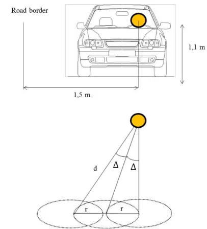
The segmented road is used to define the position of the point of view of the driver. According to regulation (Ministerio de Fomento 1999), the point of view of the driver is fixed in a distance of 1.5 m from the external border of the lane to the car (Figure 2).
3.2 Visibility analysis
The visibility analysis is based on a ray-tracing algorithm, which consist on creating a Line of Sight (LOS) from one point to an objective point, and check the obstacles causing trajectory. The LOS rotates counter clockwise around the vertical axis through the field of peripheral vision (Figure 1), forming an angle of ±60º with the centred LOS (dotted line) (Bhise, 2011).
Figure 1. Peripheral vision angle centred in the position of the driver eyes.
LOS rotation is carried out by varying a rotation angle in the horizontal plane as the algorithm detects an occlusion (Figure 2).
Figure 2. Image with radial buffer step angle representation.
The angle of rotation of the LOS around the Z axis is determined in order to ensure the whole field of view is The International Archives of the Photogrammetry, Remote Sensing and Spatial Information Sciences, Volume XLI-B1, 2016
scanned. Based on the information provided by the Dirección General de Tráfico (DGT 2015), a car speed of 100 km/h stops in a distance of 150 m. Thus, the maximum distance to occlusion is fixed as 150 m. Occlusion detection is performed searching points on the 3D model in a cylinder around the LOS with a radius (r) of 0.25 m. Authors consider that a cylinder of 0.5 m diameter of vision should be enough to detect a person. As a result, a polyline is formed with the occlusions detected by the algorithm. Projecting this area onto the XY plane, a surface is defined and it corresponds with the area of visibility available from one point of the driver trajectory (Figure 3).
The projection takes into account only x and y components of the points detected as occlusions. The area of the polygon is calculated utilizing the Gauss formula in the 2D projected line, where u and v are the vectors with the x and y components of the list of vertex of the polygon, respectively. The number of vertexes are represented by n, taking the position of the vehicle as first and last vertex. All the algorithms developed for this work have been implemented in MatLAB software.
Figure 3. Plane projection of the occlusion points and area obtained.
3.3 Occlusion detection
In the proposed approach, occlusion is defined as the existence of a determined number of points of the 3D model that interrupt the LOS between the driver and the object that needs to be seen. There could be some points in the model that are not defining a real element of the road or that belong to an object that has not the volume enough to behave as an actual obstacle. Therefore, it is needed to define a condition to consider when the occlusion detected in the model can be considered as a real obstacle for occluding vision of an obstacle.
A cylindrical volume is created around each LOS. The algorithm checks if there are points of the point cloud inside the cylinder. In the case a point is detected inside the cylinder, it is needed to know if it is an isolated point or a cluster of points. An isolated point does not affect to visibility. However, a cluster of points contributes negatively to visibility. Thus, occlusion detection depends on the local density of the 3D model. The number of points in the surroundings is evaluated in the volume where the point detected is located. This local
density is calculated as the number of points of the model that are inside of a sphere with centre in the LOS and with the radius fixed in buffer radius. Figure 4 shows an example of the occlusion condition algorithm.
Figure 4. Different conditions in the occlusion for the algorithm.
To summarize, it can be said that the existence of an occlusion in the model is defined as the existence of n points of the point cloud inside a sphere of a 0.5 m radius with the centre in any point along the LOS. The election of the number of points that should be inside the sphere to consider it an occlusion determines the resulting visibility area (Figure 5).
Figure 5. Different conditions in the occlusion for the algorithm. Visibility up to 150 m is considered. Black arrow
indicates the direction and position of the car.
3.4 Correction based on weather conditions
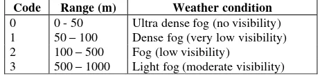
The visibility results are corrected using the following table, extracted from data provided by the Spanish Meteorological Agency (AEMET, 2016) and the Galician Weather Agency (Meteogalicia, 2016). The correction actuates on the measurement range length, limiting the value to the maximum provided by the weather conditions.
Code Range (m) Weather condition
0 0 - 50 Ultra dense fog (no visibility) 1 50 – 100 Dense fog (very low visibility) 2 100 – 500 Fog (low visibility)
3 500 – 1000 Light fog (moderate visibility)
Table 1. Fog relation with visibility range. The International Archives of the Photogrammetry, Remote Sensing and Spatial Information Sciences, Volume XLI-B1, 2016
4. RESULTS AND DISCUSSION
4.1 Data sources
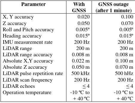
A mobile LiDAR system Optech Lynx mobile mapper (Figure 6) is used for the data acquisition. The Lynx main components are GNNS/IMU unit for navigation (Applanix POS LV 520) and two LiDAR sensors for range measurement. Table 2 shows the main technical specifications of the system.
Figure 6. Mobile LiDAR Optech Lynx.
Parameter With GNSS
GNSS outage (after 1 minute)
X, Y accuracy 0.020 0.100
Z accuracy 0.050 0.070
Roll and Pitch accuracy 0.005º 0.005º
Heading accuracy 0.015º 0.015º
IMU measurement rate 200 Hz 200 Hz
LiDAR range 200 m 200 m
LiDAR range accuracy 0.008 m 0.008 m Absolute X,Y accuracy 0.022 m 0.100 m
Absolute Z accuracy 0.050 m 0.070 m
LiDAR pulse repetition rate 500 kHz 500 hHz
LiDAR scan frequency 200 Hz 200 Hz
LiDAR echoes ≤ 4 ≤ 4
Operation temperature -10 ºC to + 40 ºC
-10 ºC to + 40 ºC
Table 2. Technical specifications of Optech Lynx mobile LiDAR.
The methodology is tested in two different data sources, an urban road in the city of Vigo (Figure 7) and an inter-urban road between the city of Ourense and the village of Castro Caldelas (Figure 8), both in Spain.
Figure 7. Point cloud of the urban road in Vigo.
Figure 8. Point cloud of the inter-urban road between Ourense and Castro Caldelas.
4.2 Optimization of rotation angle
The algorithm proposed for visibility analysis is sensitive to a number of parameters. In order to check the sensibility to the rotation angle , the algorithm has been run with different values. Results show that an angle of 0.1º does not show important differences with the minimum angle studied 0.01º. Variations of the angle under 0.01º do not affect the result of the algorithm, so they are not studied (Figure 9).
Figure 9. Different curves representing the area of visibility in function of the occlusion condition.
4.3 Visibility diagrams
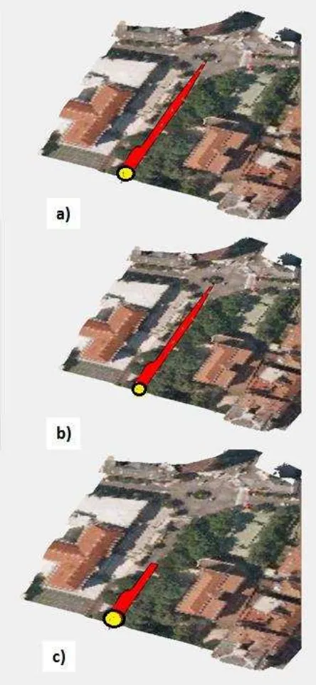
Figure 10 shows the visibility diagram for the first case study (urban road in Vigo). The algorithm shows a reliable behaviour in the detection of cars parked on the road side, the poles, and trees that could affect to driver visibility. In addition, the reduction of visibility produced by meteorological events as fog is introduced in the algorithm and represented on the graphs. The algorithm does not present spurious detected points.
Figure 10. Case study 1. Visibility diagram in the urban road in Vigo. Yellow circle indicates the car position. Visibility range: a) 150 m (fog), b) 100 m (dense fog), and c) 50 m (ultra dense
fog).
Figure 11 exhibits the visibility diagram for the second case study (inter urban road between Ourense and Castro Caldelas). It also shows a reliable result, similar to that obtained in the first case study.
Figure 11. Case study 2. Visibility diagram in the inter urban road between Ourense and Castro Caldelas. Yellow circle indicates the car position. Visibility range: a) 150 m (fog), b)
100 m (dense fog), and c) 50 m (ultra dense fog).
5. CONCLUSIONS
An algorithm to the evaluation of visibility in roads is developed. It is based on ray tracing previous results. The algorithm includes a correction based on the weather conditions. The step angle used for the ray tracing is 0.01º and the density of points 50 points/m3. The methodology is tested in two case studies, an urban and an inter-urban road. In both cases the visibility diagrams are reliable. No spurious points are founded.
ACKNOWLEDGEMENTS
Authors want to give thanks to the Xunta de Galicia and Govierno de España for the Grants CN2012/269, TIN2013-46801-C4-4-R, and ENE2013-48015-C3-1-R.
REFERENCES
AEMET, 2016. Available at: http://www.aemet.es/es/portada (last access 01/04/2016)
Alsadik, B., Gerke, M., Vosselman, G., 2014. Visibility analysis of point cloud in close range photogrammetry. ISPRS Annals of Photogrammetry, Remote Sensing and Spatial Information Sciences, 5, pp. 9 – 16. modelling for sight distance studies. Survey Review.
DGT. 2015. Revista Tráfico y Seguridad Vial, N224. Available
at:
<http://asp-es.secure-zone.net/indexPop.jsp?id=5938/10033/23388&startPage=1&lng =es#5938/10033/233881es> (last access 01/04/2016)
Dumbaugh, E., Wenhao, L., 2010. Designing for the safety of pedrestrians, cyclists and motorists in urban environments. Journal of the American Planning Association, 77(1), pp. 69 – 88.
Hassan, Y., Easa, S., El Halim, A., 1996. Analytical model for sight distance analysis on three-dimensional highway alignments. Transportation research record: Journal of the transportation research board, 1523, pp. 1 – 10.
Liu, X., Zhang, Z., Peterson, J., Chandra, S., 2007. The effect of LiDAR data desity on DEM accuracy. Proceedings of the International Congress on Modelling and Simulation, pp. 1363 – 1369.
Meteogalicia, 2016. Available at: http://meteogalicia.es (last access 01/04/2016)
Mertzanis, F. S., Boutsakis, A., Kaparakis, I. G., Mavromatis, S., Psariaos B., 2015. Analytical method for 3D stopping sight distance adequacy investigation. Journal of Civil Engineering and Architecture, 9(2), pp. 232 – 243.
Ministerio de Fomento. 1999. Trazado: Instruccion de caretera.
Norma 3.1-IC. Available at:
http://www.fomento.gob.es/NR/rdonlyres/7CDCD3E7-850A-4A9C-813D-B87FAEDE1A7A/55858/0510100.pdf (last access 01/04/2016)
Puente, I., González-Jorge, H., Martínez-Sánchez, J., Arias, P., 2013. Review of mobile mapping and surveying technologies. Measurement, 46(7), pp. 2127 – 2145.
Puente, I., González-Jorge, H., Martínez-Sánchez, J., Arias, P., 2014. Automatic detection of road tunnel luminaires using a mobile LiDAR. Measurement, 47, pp. 569 – 575.
Riveiro, B., González-Jorge, H., Martínez-Sánchez, J., Arias, P., 2015. Automatic detection of zebra crossings from mobile LiDAR data. Optics and Laser Technology, 70, pp. 63 – 70.
Serna, A., Marcotegui, B., 2013. Urban accessibility diagnosis from mobile laser scanning data. ISPRS Journal of Photogrammetry and Remote Sensing, 84, pp. 23 – 32.
Tarel, J., Charbonnir, P., Goulette, F., Deschaud, J., 2012. 3D road environment modelling applied to visibility mapping: An experimental Comparison. IEEE/ACM 16th International
Symposium on Distributed Simulation and Real Time Applications, pp. 19 – 26.
Tomljenovic, I., Rousell, A., 2014. Influence of point cloud density on the results of automated object-based building extraction from ALS data. AGILE Digital Editions. Available at: <http://repositori.uji.es/xmlui/handle/10234/98911> (last access 01/04/2016)
Ural, S., Shan, J., Romero, A., Tarko, A., 2015. Road and roadside feature extraction using imagery and LiDAR data for transport operation. ISPRS Annals of Photogrammetry, Remote Sensing and Spatial Information Sciences, 3, pp. 239 – 246. Varela-González, M., González-Jorge, H., Riveiro, B., Arias, P., 2014. Automatic filtering of vehicles from mobile LiDAR datasets. Measurement, 53, pp. 215 – 223.
Yang, B., Fang, L., Li, J., 2013. Semi-automated extraction and delineation of 3D roads of street scene from mobile laser scanning point clouds. ISPRS Journal of Photogrammetry and Remote Sensing, 79, pp. 80 – 93.
Yin, C. L., Wen, Q. X., Qing, M. Z., Hong, H Z., 2012. Visibility analysis for three-dimension urban landscape. Key Engineering Materials, 500, pp. 458 – 464.