Analysis of maize growth for different irrigation strategies
in northeastern Spain
I. Farre´
a,b,*, M. van Oijen
c,d, P.A. Leffelaar
c, J.M. Faci
aaDepartment of Soils and Irrigation,Ser6icio de In6estigacio´n Agroalimentaria(DGA),PO Box727,50080Zaragoza,Spain bCSIRO Plant Industry,Pri6ate Bag No.5,Wembley,Western Australia,6913,Australia
cDepartment of Theoretical Production Ecology(WAU-TPE),Wageningen Agricultural Uni6ersity,PO Box430,
6700AK Wageningen,The Netherlands
dInstitute for Terrestrial Ecology(ITE),Edinburgh Research Station,Penicuik EH26OQB,UK
Received 3 June 1998; received in revised form 29 November 1999; accepted 31 January 2000
Abstract
Water availability is the key factor determining maize yields in NE Spain. Irrigation is needed to obtain economic yields but it is costly and water supply is sometimes insufficient. The aim of this research was to test a simple simulation model for evaluating different irrigation strategies, especially under water-limited conditions. The LINTUL model was adapted and parameterized using experimental data from the 1995 season. Most parameters were obtained from experiments, although some were taken from the literature. This model is based on the concept of light use efficiency, incorporates a soil water balance and simulates phenology, crop leaf area, biomass accumulation and yield. It was tested on independent data from the 1995 and 1996 seasons under different irrigation treatments. The model predicted the flowering date within 95 days of the observed values. Leaf area index was predicted satisfactorily, except under extreme water-stress conditions, where it was overestimated. In general, soil moisture content and yield were accurately predicted. In the 1996 experiment measured yields ranged from 6.4 to 13.6 t ha−1and simulated yields from 6.5 to 12.2 t ha−1. These results show that the LINTUL model can be used as a tool for exploring the consequences on maize yields of different irrigation strategies in NE Spain. Analysis of the model identified a process that strongly affects yield loss due to drought, but for which present understanding is still insufficient: the effects of drought on leaf senescence and canopy architecture. © 2000 Elsevier Science B.V. All rights reserved.
Keywords:Maize; Irrigation; Water stress; Simulation model
www.elsevier.com/locate/euragr
1. Introduction
Maize (Zea maysL.) is one of the major
sum-mer crops grown in the Mediterranean region. The scarce and highly variable precipitation in this region makes efficient planning of water use * Corresponding author. Tel.:+61-8-9333-6789; fax:+
61-8-9387-8991.
E-mail address:[email protected] (I. Farre´)
for irrigation necessary for most summer crops. Extensive research has been carried out on crop responses to water-limited conditions. Maize has been reported to be very sensitive to drought, particularly during flowering (Begg and Turner, 1976; Otegui et al., 1995). NeSmith and Ritchie (1992a) reported yield reductions exceeding 90% caused by water-deficit during flowering in maize. The degree of yield reduction is determined by the is timing, severity and duration of the water deficit (Hsiao, 1990). It is difficult to plan a deficit irrigation scheme for maize without causing yield reductions (Rhoads and Bennett, 1990; Lamm et al., 1994).
To determine optimal irrigation strategies one could choose to do a large number of site-specific, long-term experiments. However, field experi-ments are time consuming and costly. Another option, therefore, is to integrate our present un-derstanding of the processes responsible for crop response to water availability in crop simulation models. In this way the number of field experi-ments is reduced, while the model may be used in an exploratory manner to assess irrigation scenar-ios that can not be economically evaluated by experimentation and thus help improve irrigation management.
Several crop models have been developed for crop-water relationships differing in approach and detail (Jones and Kiniry, 1986; Spitters and Schapendonk, 1990; Amir and Sinclair, 1991; Jef-feries and Heilbronn, 1991; Muchow and Sinclair, 1991; Stockle et al., 1994). The level of complexity
required depends on the aims of the model. Sim-ple models are often appropriate when aiming for yield prediction (Maas, 1993). Such simple models are more easily parameterized and often show a more robust behaviour than complex models. In this paper complexity of the model is kept to a minimum and additional phenomena or processes were only incorporated if they were expected to improve the predictive ability of the model.
For this purpose, we have selected the generic crop growth model LINTUL, which calculates crop growth as the product of light interception and light use efficiency, and includes a water balance (Spitters and Schapendonk, 1990).
The objectives of this paper were to parameter-ize and test the LINTUL model, in order to develop a tool for exploring the consequences for maize yield of different irrigation strategies in the dry conditions of the Ebro Valley in northeast Spain. For model parameterisation and testing, we carried out field experiments in the region, in which drought was imposed at various times and various severities.
2. Field experiments
Three experiments (Table 1) were conducted in
Zaragoza, northeast Spain (latitude 41° 43% N,
longitude 0° 49% W, altitude 225 m) during the
growing seasons of 1995 and 1996, to study the response of maize (cv. Prisma 700) to water deficits. The soil, developed from alluvial deposits,
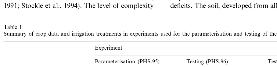
Table 1
Summary of crop data and irrigation treatments in experiments used for the parameterisation and testing of the LINTUL modela
Experiment
Parameterisation (PHS-95) Testing (PHS-96) Testing (CS-95)
145 146
145 Crop emergence date (DOY)
Plant density (pl m−2) 8.2 8.0 8.2
0.75
Row spacing (m) 0.75 0.75
275 290
278 Harvest date (DOY)
III, Is%I, IsI, sII,
Irrigation treatments III, IIs, IsI, sII, T1, T2, T3,
Iss, ssI, sIs, sss, rrr
Iss, ssI, sIs, sss, rrr T4, T5, T6
aDates are expressed in day of the year (DOY). CS, continuous stress experiment; PHS, phases stress experiment. The different
was classified asTypic Xeroflu6ent. The depth that may be rooted is determined by a gravel layer occurring between 1.0 and 1.7 m. The texture is sandy loam in the 0.0 – 0.5 m top soil and loam to sandy loam below. The volumetric moisture con-tent at field capacity (0.03 MPa) and permanent wilting point (1.5 MPa) in each 0.3 m layer to 0.9 m depth were measured using pressure plates (Richards, 1949). The values of field capacity and wilting point hardly differed in the three measured layers in the 0 – 0.9 m soil profile, and were aver-aged as 27 and 9%, respectively.
Soil water content was monitored gravimetri-cally and/or by neutron probe in each 0.2 or 0.3 m layer down to 1 – 1.2 m depth during the growing season. The average moisture content of the profile used for comparison with the model was calculated from the soil water contents in each layer up to 0.9 m depth, taking into account the layer thickness. Experimental details are given in Table 1. Crop development was recorded from emergence to physiological maturity. Plant height and the fraction of photosynthetically active radia-tion (PAR) intercepted by the crop were measured at 1- to 2-week intervals. Intercepted PAR (IPAR) was calculated from PAR values that were mea-sured below and above the crop canopy with a portable tube solarimeter (Model Delta T-Devices Ltd). To eliminate the effect of solar altitude on the interception values the measurements were taken at noon on cloudless days. Leaf area index (LAI) and specific leaf area (SLA) were measured at flowering. Shoot biomass and its partitioning among the different plant organs was determined
biweekly by harvesting 0.5 m2from each plot. At
physiological maturity, total above ground
biomass and grain yield was obtained.
Electrical conductivity of 1:5 soil – water extracts (ECs) was measured to assess possible salinity problems during the experimental period. Cultural practices comprise high input conditions to avoid nutritional limitations. Weeds, insects and diseases were controlled according to common practices in the area.
Irrigation scheduling for the well-irrigated treat-ments was calculated from the reference
evapo-transpiration (ET0) measured in a weighing
lysimeter located nearby multiplied with a
time-de-pendent crop coefficient (Doorenbos and Pruitt, 1977). Rainfall during the growing season was 35 mm in 1995 and 103 mm in 1996, which represents 5 and 16% of the total crop water requirements, respectively.
2.1. Water stress during different growth phases (phases stress experiments=PHS)
Field experiments were carried out in 1995 and 1996 to study the effects of a moderate water stress at different stages of crop development in maize. The growing season was divided into three phases: (1) from emergence to tassel emergence; (2) from tassel emergence to milk stage of grain; and (3) from milk stage to physiological maturity. In each of the phases either irrigation to meet the potential evapotranspiration of the crop (I) or about one third of this amount (s) was supplied, by skipping some of the irrigation events or apply-ing a lower depth. All possible combinations of these treatments were applied (III, IIs, IsI, sII, Iss, ssI, sIs, sss). An additional treatment (rrr), consist-ing of half of the water used in the well-irrigated treatment, was included. Irrigation management in the well-irrigated treatment was based on the common irrigation practices in the area, which consist in flood irrigation at 10 – 14 days interval. The experimental design was a randomised block, with nine treatments and three blocks. Soil
ridges delimited plots of 50 m2. Irrigation was
applied from 200 mm diameter gated pipes with a total discharge rate in each plot of 3.4 l s−1. Total
water applied at each irrigation was measured with a volumetric flow meter. The depth of water applied in each irrigation varied from 32.0 to 79.3 mm. The III treatment received a total of nine and eight irrigations during the growing season in 1995 and 1996, respectively. The rest of the treatments received between three and seven irrigations (Table 2).
2.2. Continuous water stress experiments (continuous stress experiment=CS)
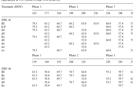
sprin-Table 2
Irrigation dates (day of the year, DOY) and amount of water applied (mm) in the different irrigation treatments in the phases stress experiments in 1995 (PHS-95) and 1996 (PHS-96).
Phase 2
Treatment (DOY) Phase 1 Phase 3 Total
177 188 199 209 218
165 234 248 262
PHS-95
65.2 60.7 60.2 65.0 65.0
79.3 60.0
III 57.4 55.6 568.4
65.2 60.7 60.2
Is%Ia 79.3 60.0 57.4 55.6 438.4
65.2 60.7 52.0
79.3 60.0
IsI 57.4 55.6 430.2
65.2 60.2
sII 65.0 65.0 60.0 57.4 55.6 428.4
65.2 60.7 52.0
79.3
Iss 57.4 314.6
65.2 52.0
sII 60.0 57.4 55.6 290.2
65.2 60.2 65.0 65.0
sIs 57.4 312.8
sss 65.2 52.0 57.4 174.6
60.7 65.0
79.3 60.0
rrr 55.6 320.6
Phase 1 Phase 2 Phase 3
159 180 192 204 218 229 243 257
PHS-96
58.4 69.7 70.7 66.0 55.2 59.7 62.4 505.3
III 63.3
58.4 69.7 70.7 66.0 63.3
IIs 59.7 387.8
58.4 69.7 32.0 55.2 59.7 62.4 400.6
IsI 63.3
58.4 70.7 66.0 55.2
sII 59.7 62.4 372.2
58.4 69.7 32.0
Iss 63.3 59.7 283.1
58.4 32.0 55.2
ssI 59.7 62.4 267.5
sIs 58.4 70.7 66.0 59.7 254.7
58.4 32.0
sss 59.7 150.0
69.7
rrr 63.3 66.0 59.7 258.7
aIn 1995 two treatments were subjected to deficit irrigation in phase 2: the IsI received one irrigation in the middle of phase 2,
whereas the Is%I treatment received one irrigation at the beginning of phase 2.
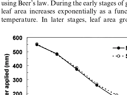
kler line-source provided adequate water near the sprinkler line throughout the growing season while applying a decreasing quantity of water with increasing distance perpendicular to the line-source. To define different irrigation treatments the gradient of water applied was divided into six parts (T1 – T6). Water stress developed progres-sively during the growing season in the five sub-optimal irrigation treatments (T2 – T6). Irrigation was applied every 2 – 4 days to meet the potential evapotranspiration demand of a maize crop at the rows nearest to the line source (T1). Catchment cans installed across the field at a spacing of 2.25 m were read after each irrigation. The degree of deficit irrigation for each treatment can be in-ferred from Fig. 1, is which shows the amount of water applied to the different treatments during
the growing season. A total of 27 irrigations were applied during the irrigation season. The total seasonal amount of irrigation water applied in T1 was 551.2 min.
3. Model description
charac-teristic time coefficient of the model. A code listing is available upon request from the authors of the paper.
Required inputs for the model include daily weather data (maximum and minimum tempera-ture, global radiation, rain, vapour pressure and wind speed), crop management data (plant density and day of emergence), crop parameters, the soil moisture retention characteristics (soil water con-tent at saturation, field capacity, wilting point and air dryness) and the initial soil water content.
The model consists of two major parts, the plant growth component and the soil water component, which may induce a reduction in growth rate.
3.1. Crop growth under optimal water supply
The dry weights of the different plant organs (leaves, stems, roots and grains) are the state variables in the crop growth model and are ob-tained by integration of their growth rates is over time. The daily crop biomass increment is calcu-lated as the product of the amount of IPAR by the crop and the light use efficiency (LUE). In the absence of drought, LUE is constant. Light inter-ception by the crop is modelled as a function of its LAI and a constant light extinction coefficient (K), using Beer’s law. During the early stages of growth, leaf area increases exponentially as a function of temperature. In later stages, leaf area growth is
calculated as the increase in leaf weight times a constant specific leaf area. Leaf senescence due to ageing and self-shading is taken into account in computing the net increase in leaf weight. The dry matter produced is partitioned among the various plant organs, using partitioning factors defined as a measured function of the thermal time. For example, grain yield is calculated as total dry matter growth multiplied by the thermal-time de-pendent fraction of dry matter allocated to the storage organs.
3.2. Effects of drought on crop growth
In the model, water-limiting conditions have two effects on the crop: reduction of growth rate and change in allocation pattern. Crop growth is re-duced proportionally via the ratio of actual to potential transpiration. The critical soil water con-tent below which transpiration rate is reduced below its potential value depends on crop sensitiv-ity to drought and the evaporative demand of the atmosphere (Driessen, 1986). Dry matter partition-ing changes in favour of root growth durpartition-ing the vegetative phase (Munns and Pearson, 1974) when the ratio of actual to potential transpiration falls below 0.5 (Van Keulen et al., 1981). No effects of
drought on crop morphology (K, SLA) and leaf
senescence are assumed in the model.
3.3. Soil water balance
Soil water balance is calculated using one soil layer, which increases in thickness depending on root depth (Van Keulen, 1986). Root growth causes exploration of the water in depth, until the maxi-mum rooting depth or soil depth is reached. Newly explored soil depth is assumed to be at field capacity initially. The daily change in soil moisture content in the rooting zone is calculated as the net result of water gain from irrigation and rainfall, minus water loss by crop transpiration, soil evapo-ration, runoff and deep percolation. Daily values of irrigation and rainfall are inputs needed in the model. Percolation is calculated as the amount of water in excess of field capacity that drains below the root zone. Runoff occurs if maximum drainage capacity is exceeded.
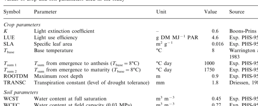
Table 3
Values of crop and soil parameters used in the study
Unit Value Source
Symbol Parameter
Crop parameters
– 0.6 Boons-Prins et al., 1994 K Light extinction coefficient
g DM MJ−1PAR 4.6
Light use efficiency Exp. PHS-95
LUE
m2 g−1 0.016
SLA Specific leaf area Exp. PHS-95
°C 8
Base temperature Warrington and Kanemasu,
Tbase
1983 Tsum 1 Tsumfrom emergence to anthesis (Tbase=8°C) °C day 1000 Exp. PHS-95
°C day 1750 Exp. PHS-95 Tsum 2 Tsumfrom emergence to maturity (Tbase=8°C)
m 0.9
Maximum root depth Exp. PHS-95
ROOTDM
TRANSC Transpiration constant (level of drought tolerance) mm 1.8 Driessen, 1986
Soil parameters
m3 m−3 0.45
WCST Water content at full saturation Exp. PHS-95
m3 m−3 0.27
Water content at field capacity (0.03 MPa) Exp. PHS-95 WCFC
m3 m−3 0.09 Exp. PHS-95
WCWP Water content at wilting point (1.5 MPa)
m3 m−3 0.03 Exp. PHS-95
Water content at air dryness WCAD
Potential evapotranspiration is calculated with the Penman equation (Penman, 1948). Potential transpiration is a fraction of this rate, equal to
fractional light interception calculated using
Beer’s law. The ratio of maize transpiration to Penman transpiration is introduced in the model to obtain the potential maize transpiration. This ratio ranges from 1.0 to 1.2 depending on ground cover (Doorenbos and Pruitt, 1977). Actual tran-spiration rate is calculated from its potential value and the soil water status. Actual evaporation is calculated from its potential value, the soil water status and an additional exponential decrease af-ter days without rain or irrigation. The exponen-tial decrease is a simplified implementation of Ritchie’s concept of evaporation reduction pro-portional to the square root of the number of days since the last rainfall with a fixed wet stage of 1 day (Ritchie, 1972).
4. Model parameterisation
A part of the experimental data was used for parameterisation of the model, whereas another independent portion of the data was reserved to test the model. Experiment PHS-95 was chosen for model parameterisation because it had a high
frequency of detailed field measurements. Values that could not be obtained from this experiment were taken from the literature. A list of the crop and soil parameters, resulting from the parameter-isation described below, with their values is sum-marised in Table 3.
4.1. Crop parameters
4.1.1. Light extinction coefficient
Extensive measurements on spring wheat cv. Yecora 700 24 (Robertson and Giunta, 1994), had revealed no effects of drought on the light extinc-tion coefficient. In contrast, in our own experi-ments light extinction measured at noon at
anthesis (whenKhas the lowest value) was found
to be affected by the different irrigation
treat-ments (K — fully irrigated, 0.5; K — deficit
irrigation, 0.2 – 0.3). Extensive measurements (di-urnal and over the season) would be needed to allow a parameterisation of the effect of drought
on K. In the model, due to lack of experimental
data, K was assumed to be constant throughout
4.1.2. Light use efficiency
LUE was obtained by simple linear regression of total crop biomass, measured at different times in the season, and cumulative light interception,
in the well-irrigated treatment. Total crop
biomass was computed as the sum of measured
above ground biomass and estimated root
biomass. Root biomass was estimated using the observation that the ratio of root growth to total
growth decreases from 0.5 to 0 from emergence to anthesis (Penning de Vries et al., 1989).
Daily total incident PAR was multiplied by the fraction of light that was intercepted (values be-tween measurements were linearly interpolated) to obtain the daily IPAR by the crop. The sum of these daily values gave the total cumulative IPAR by the crop. LUE was then calculated as the slope of the regression line of cumulative total crop biomass on cumulative IPAR (Fig. 2). The regres-sion line was forced through the origin, because of the assumed direct proportionality of light inter-ception and growth. Post-anthesis harvests were excluded because of unmeasured weight loss due
to fallen leaves. A value of LUE of 4.6 g DM/MJ
IPAR was obtained. A similar value (4.5) has been found by Cabelguenne et al. (1990) in south-ern France. Lower values have been reported for
maize in different experiments (3.5 g MJ−1,
Maas, 1993; 4.0 g MJ−1
, Stockle et al., 1994) but these values refer only to above ground biomass. Values obtained in the literature agree well with
the value of 3.8 g MJ−1
found in our experiment when only above ground biomass was considered (Fig. 2).
4.1.3. Dry matter partitioning
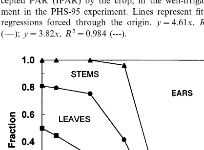
Partitioning of the daily increment of dry mat-ter among leaves, stems, roots and storage organs was related to thermal time (Fig. 3). Thermal time was calculated (Table 3) with a base temperature of 8°C (Warrington and Kanemasu, 1983; Ca-belguenne et al., 1990). Roots were not measured in the field experiment. Partitioning between shoot and root was therefore, assumed to be similar to earlier reports (Penning de Vries et al., 1989; Boons-Prins et al., 1994). The pattern of allocation to leaves, stems and storage organs was derived as the fraction of new above-ground biomass production allocated to the different plant organs between two subsequent harvests (Fig. 3). This above-ground allocation pattern hardly varied among treatments. Decreases in leaf and stem weight at late growth stages due to senescence and translocation were assumed to in-dicate that no more biomass was allocated to these organs.
Fig. 2. Relationship between cumulative dry matter (total crop biomass and above-ground biomass) and cumulative inter-cepted PAR (IPAR) by the crop, in the well-irrigated treat-ment in the PHS-95 experitreat-ment. Lines represent fitted linear regressions forced through the origin. y=4.61x, R2=0.995
( — );y=3.82x,R2=0.984 (---).
Fig. 4. Measured (symbols) and calculated (lines) leaf area index (LAI) values in treatments III, rrr and sss of the PHS-95 experiment.
rigated treatment, was used in the model. The same value has been reported for maize (Sibma, 1987). No effect of water stress on SLA is consid-ered in the model.
4.1.5. Leaf senescence
Water stress can accelerate leaf senescence (Ne-Smith and Ritchie, 1992b). Despite the differences in leaf senescence visually assessed among treat-ments in the field experitreat-ments, lack of quantita-tive data did not allow us to establish a relationship between leaf senescence and irriga-tion treatment. In the model leaf senescence oc-curs due to ageing (through temperature and thermal time) and due to shading (through LAI), but the effect of water stress on leaf senescence is not considered.
4.2. Soil parameters
Soil water content at field capacity (0.27 m3
m−3) and wilting point (0.09 m3 m−3) were
ob-tained using pressure plates (Richards, 1949). Soil
water content at saturation (0.45 m3
m−3
) was estimated from porosity measurements and at air
dryness (0.03 m3 m−3) as one third of wilting
point.
4.3. E6aluation of the model parameterisation
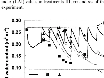
The parameterisation was checked first by run-ning the model for the conditions of the PHS-95 experiment. The calculated LAI satisfactorily matched the measured values from the experiment for different treatments except for the treatment subjected to deficit irrigation during all of the three developmental phases (sss), where LAI was overestimated (Fig. 4). Fig. 5 shows the averaged measured and simulated soil water content of the total profile for the treatments HI, rrr and sss at several dates during the crop season. Soil water content was simulated accurately at the end of the crop season. Throughout the season the predicted soil water content did not exactly match the mea-sured values from the experiment, but the experi-mental data were included in the general trend of data.
Fig. 5. Measured (symbols) and calculated (lines) volumetric soil water content in the 0 – 0.9 m soil profile in treatments III, rrr and sss of the PHS-95 experiment. Horizontal lines repre-sent sod water content at field capacity (FC) and wilting point (WP).
4.1.4. Specific leaf area
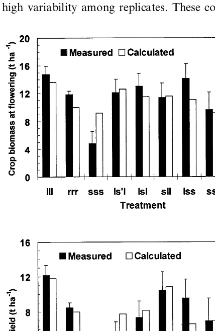
well-ir-Fig. 6 shows the measured and calculated above-ground biomass at anthesis (Fig. 6a) and yield at maturity (Fig. 6b) for all the treatments of the PHS-95 experiment. The model correctly showed the trend of yield reduction under a de-creasing amount of irrigation applied. In general, good agreement was observed between measured and calculated yields, differing on average by 23%. In six out of nine treatments the differences between the calculated and the observed values were within 5%, but deviations for the remaining
three treatments (sss, Is%I and Iss) amounted to
60% and were significant. Measured yields had a high variability among replicates. These
compari-Fig. 7. Measured (symbols) and simulated (lines) leaf area index (LAI) in treatments III, rrr and sss of the PHS-96 experiment for model testing.
Fig. 6. Measured and calculated above ground biomass at flowering (a) and final yield (b) in all treatments of the PHS-95 experiment. Yield (oven dried weight) is expressed as the whole ear (grain+cob). For treatment details see text. Vertical lines represent the standard errors of the mean (S.E.).
sons provide some information about the reason-ableness of the model structure. It is however, not an independent model test. Testing of the model on independent data is described in the next section.
5. Model testing
After parameterisation the model was tested against independent data from the CS-95 and PHS-96 experiments (Table 1). The model was tested with respect to: date of flowering, leaf area index, soil water content, crop biomass and yield. The date of flowering was simulated within 2 days of the observed dates in the well-irrigated treatments. In the water-deficit treatments, flower-ing was delayed between 2 and 5 days compared with the model results. This delay was not pre-dicted by the model, because it assumes phenol-ogy to be only dependent on thermal time, so effects of water stress on phenology are not taken into account. However, in maize, water deficit can delay anthesis and physiological maturity. Ne-Smith and Ritchie (1992a) reported a delay in anthesis of up to 15 days in maize grown under water-limited conditions.
experi-ment, for the III, rrr and sss treatments. Up to 45 days after sowing (day of year (DOY), 183), LAI was simulated well for all the treatments, and for the rest of the season it was simulated satisfacto-rily in the well-irrigated treatments. In the deficit irrigation treatments, increased leaf senescence as a result of water stress caused LAI to decrease. Because the model does not account for the effect of water deficit on leaf senescence, LAI from 45
days after sowing was overpredicted. In the CS-95 experiment, the LAI was also overestimated for all the suboptimal irrigation treatments (T2 to T6; data not shown).
Measured and simulated soil water content at different dates were compared for the treatments III, rrr and sss in the PHS-96 experiment (Fig. 8). The measured soil water content data were in-cluded in the general trend of the model, but given the scarcity of the data no final conclusion can be extracted.
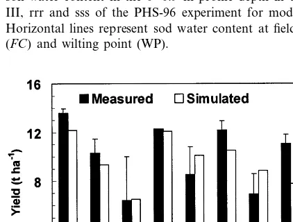
Measured and simulated yields and dry matter at maturity were compared for all the irrigation treatments of the PHS-96 and CS-95 experiments. The model correctly showed the trend of yield reduction under decreasing irrigation amounts. In the PHS-96 experiment, measured yields ranged
from 6.4 to 13.6 t ha−1and simulated yields from
6.5 to 12.2 t ha−1 in the different irrigation
treatments (Fig. 9). Mean measured and simu-lated yields were 10.4 and 9.7 t ha−1, respectively.
Lowest yields were obtained in the sss treatment,
both measured (6.4 t ha−1) and simulated (6.5 t
ha−1). Actual and simulated above-ground
biomass had a similar relative magnitude of varia-tion (data not shown). The model accurately esti-mated yields for the treatments subjected to: full irrigation (III), moderate water deficit (rrr) and severe water deficit (sss) during the three phases of the growing season (measured and simulated dif-fering by 7%). However, grain yield was overesti-mated (measured and simulated differing by 25%) for the treatments subjected to deficit-irrigation during the flowering phase. In contrast, in the treatments with limited-irrigation during the vege-tative phase, grain yield was underestimated (mea-sured and simulated differing by 21%), irrespec-tive of the amount of irrigation received at later stages.
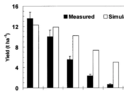
In the CS-95 experiment (Fig. 10) the model correctly simulated the observed trend of yield reduction under the gradient of water applied, but the simulated decrease in yield was less pro-nounced than observed. Measured yields
de-creased from 13.6 t ha−1 in the well-irrigated
treatment (T1) to almost none (0.1 t ha−1) in the
least irrigated treatment (T6). The model
pre-dicted a range of yields from 12.3 to 2.5 t ha−1
Fig. 8. Measured (lines) and simulated (symbols) volumetric soil water content in the 0 – 0.9 m profile depth in treatments III, rrr and sss of the PHS-96 experiment for model testing. Horizontal lines represent sod water content at field capacity (FC) and wilting point (WP).
Fig. 10. Measured and simulated yields in all treatments of the CS-95 experiment for model testing. Yield (oven dried weight) is expressed as the whole ear (grain+cob). For treatment details see text. Vertical lines represent the standard errors of the mean (S.E.).
mm at 14-day intervals, providing a total amount
of water equivalent to half of the ETc. The
weather conditions of 1995 were used, together with an initial soil moisture content equivalent to field capacity. These scenarios provided a range of crop exposures to water deficit. Sensitivity analy-sis indicates how strongly the parameters (P) af-fect the model results and also the degree of accuracy to which the tested parameters must be known. Sensitivity coefficients (SC) are calculated as SC=(DY/Y)/(DP/P). Grain yield proved more than proportionately sensitive (sensitivity coeffi-cient SC\1); Table 4) in all scenarios to change in LUE. Sensitivity was also high but to a lesser
degree (0.5BSCB1), to leaf senescence and K.
In contrast, sensitivity of yield to change in SLA,
TRANSC and root partitioning was low (SCB
0.5) in all scenarios. Acceleration of leaf senes-cence resulted in a decrease in yield (SC negative)
in all scenarios. Increase in K resulted in an
increase in yield. Therefore, a possible decrease in
K due to water stress would lead to a decrease in
yield. The results indicate that the values of the
LUE, K and leaf senescence rate should be
accu-rately known, especially for limited irrigation conditions.
7. Discussion and concluding remarks
The results of this study reveal that the adapted LINTUL model gives satisfactory predictions of phenology, growth and yield for maize under different water conditions. The model simulates satisfactorily the time course of LAI under well-ir-rigated conditions, but overestimates it under wa-ter stress conditions. This suggests a need for studies aimed to quantifying the extent to which water stress can accelerate leaf senescence.
In the PHS-96 experiment yield was generally properly simulated, apart from an overestimation in the treatments with deficit irrigation during the flowering phase. This may be due to a particular sensitivity of maize to water stress during flower-ing. A number of studies indicate that anthesis may be a critical period for yield determination in maize (NeSmith and Ritchie, 1992a). Depending on the timing and intensity of drought, yield may for T1 to T6. The important yield reduction can
be partly explained by the combined effects of a shallow rooting pattern, high soil evaporation losses due to the high frequency irrigation and salinity on the crop in the line source sprinkler experiment. The effects of salt stress and shallow rooting system are not included in the model.
6. Sensitivity analysis
An analysis of the sensitivity of the simulated
yield to +10% changes in the input parameters
LUE, K, SLA, TRANSC (level of drought
toler-ance by the crop), root partitioning (fraction of the dry-matter partitioned to the roots as a func-tion of thermal time) and leaf senescence (rate of leaf senescence) was performed using a simulated
maize crop grown at Zaragoza at 8.2 pl m−2
. Four scenarios were evaluated, determined by the combination of two different soil types (sandy and clay soils) and two irrigation strategies (full irrigation and deficit irrigation). The full irriga-tion treatment consisted of applying irrigairriga-tion amounts of 40 mm at weekly intervals, providing a total amount of water (640 mm) equivalent to the crop evapotranspiration (ETc). The deficit
be reduced due to desynchronization of tasseling and silking, leading to impeded grain setting and kernel abortion (Struik et al., 1986). Plant adapta-tion to a moderate water stress after they had been exposed to a previous water stress could be responsible for the yield underestimation in the treatments with deficit irrigation during the vege-tative phase. In the PHS-96 experiment, limited irrigation during the vegetative phase consisted mainly of a delay in the first irrigation. The delay in the first irrigation could have enhanced root growth in early stages and caused a better ability to withstand subsequent water stress. Boyer and McPherson (1976) observed that maize grown under a non-severe water stress during the vegeta-tive period more efficiently withstood subsequent drought during the reproductive period.
A good agreement was found between simu-lated and observed yield for the well-irrigated treatment (T1) in the CS-95 experiment. The gen-eral yield overestimation for all the suboptimal irrigation treatments (T2 to T6) can be partly explained from the combined effects of a shallow rooting system and salinity in the experiments (not accounted for in the model). Data on soil water extraction during the growing season in the
CS-95 experiment showed that 70% of the plant water uptake took place from the 0.5 m top soil, 25% from the 03 – 0.7 m depth and only 5% was extracted from the 0.7 – 1.0 m depth. Even in the less irrigated treatments the crop failed to extract water from deeper soil layers. In the model, only one soil layer is considered and the maximum rooting depth is reached in all the treatments and only the total root biomass differs depending on the severity and timing of the water stress. The same rootable zone is used in the water balance for all treatments. It seems that the amount of water available to the crop was overestimated in the sprinkler irrigation experiment and therefore the effects on crop growth and yield were underes-timated.
In the CS-95 experiment, the salinity level found in the top 0.3 m at crop emergence was below the maize threshold for salinity (Rhoades et al., 1992). However, the salinity level increased progressively both across the water gradient and in time. At harvest, the soil salinity level was found to be above the crop threshold in the water stressed treatments, and thus salt stress together with the water stress can be assumed to have occurred. In these treatments irrigation was in
Table 4
Sensitivity coefficients (SC) for the model yield (Y) in two irrigation scenarios and two soil types for changes of+10% in several crop parameters (P)a
SC=(DY/Y)/(DP/P)
SLA 0.22 0.38 0.29
TRANSC −0.10 0.10 0.03 0.12
−0.16 −0.01 0.00 0.00
Root partitioning
−0.88
−1.00 −0.96
Leaf senescence −0.91
aParameters: LUE, light use efficiency;K, light extinction coefficient; SLA, specific leaf area, TRANSC, level of drought tolerance
of the crop; root partitioning (fraction of the dry-matter partitioning to the roots as a function of thermal time); leaf senescence (rate of leaf senescence).
bSixteen irrigations of 40 mm (total irrigation amount equivalent to ET c). cEight irrigations of 40 mm (total irrigation amount equivalent to half of ET
sufficient to meet the crop water requirements and to leach away soluble salts and therefore salts concentrated in the soil causing a salt stress as well as water stress in the plants. The effects of salinity on plant growth may have resulted in a reduction in the availability of water by lowering the osmotic potential (Fitter and Hay, 1987). Be-cause the model does not simulate salinity effects, this explains the lower measured yields as com-pared with the simulated yields in the water-stressed treatments.
The model has helped identifying key processes in the response of maize to deficit irrigation strategies. Important differences in K, leaf senes-cence and root patterns have been assessed among irrigation treatments in the field experiments. The sensitivity analysis has shown the high sensitivity
of the model to changes inKand leaf senescence.
Therefore, the parameterisation of the effect of
drought on K, leaf senescence and root patterns
would probably improve the model performance under water stress. However, we conclude that the simple model gives satisfactory results considering its objectives and may be used for preliminary exploration of different irrigation strategies on maize yield in the Ebro Valley.
Acknowledgements
We wish to thank Miguel Izquierdo, Jesu´s Gaudo´ and a number of friends, students and staff of the Department of Soils and Irrigation for their invaluable assistance in the field experi-ments. Financial support through the C.I.C.Y.T (Comisio´n Interministerial de Ciencia y Tecnolo-gı´a) and I.N.I.A. (Instituto Nacional de Investiga-cio´n Agroalimentaria) is gratefully acknowledged. The first author wishes to acknowledge the hospi-tality of the Department of Theoretical Produc-tion Ecology of the Wageningen Agricultural University, The Netherlands.
References
Amir, J., Sinclair, T.R., 1991. A model of water limitation on spring wheat growth and yield. Field Crops Res. 28, 59 – 69.
Begg, J.E., Turner, N.C., 1976. Crop water deficits. Adv. Agron. 28, 161 – 217.
Boons-Prins, E.R., de Koning, G.H.J., van Diepen, C.A., Penning de Vries, F.W.T., 1994. Crop specific simulation parameters for yield forecasting across the European Com-munity. Simulation reports CABO-TT 32, AB-DLO, Wa-geningen, 43 pp. and Appendices.
Boyer, J.S., McPherson, M.G., 1976. Physiology of water deficits in cereal crops. Adv. Agron. 27, 1 – 24.
Cabelguenne, M., Jones, C.A., Marty, J.R., Dyke, P.T., Williams, J.R., 1990. Calibration and validation of EPIC for crop rotation in southern France. Agric. Syst. 33, 153 – 171.
Doorenbos, J., Pruitt, W.O., 1977. Crop water requirements. FAO irrigation and drainage. Paper 24, Rome, 144 pp. Driessen, P.M., 1986. The water balance of the soil. In: Van
Keulen, H., Wolf, J. (Eds.), Modelling of Agricultural Production: Weather, Soils and Crops. Simulation Monogr. PUDOC, Wageningen, pp. 76 – 116.
Fitter, A.H., Hay, R.K.M., 1987. Environmental Physiology of Plants. Academic Press, London.
Habekotte´, B., 1997. Description, parameterization and user guide of LINTUL-BRASNAP 1.1. A crop growth model of winter oilseed rape (Brassica napus L). Quantitative Approaches in Systems Analysis 9. AB-DLO, Wageningen, 40 pp.
Hanks, R.J., Keller, J., Rasmussen, V.P., Wilson, G.D., 1976. Line source sprinkler for continuous variable irrigation-crop production studies. Soil Sci. Soc. Am. J. 40, 426 – 429. Hsiao, T.C., 1990. Measurements of plant water status. Ann.
Rev. Plant Physiol. 24, 519 – 570.
Jefferies, R.A., Heilbronn, T.D., 1991. Water-stress as a con-straint on growth in the potato crop. 1. Model develop-ment. Agric. Forest Meterol. 53, 185 – 196.
Jones, C.A., Kiniry, J.R., 1986. CERES-Maize: A Simulation Model of Maize Growth and Development. Texas A&M University Press, College Station, TX.
Lamm, F.R., Rogers, D.H., Manges, H.L., 1994. Irrigation scheduling with planned soil water depletion. Am. Soc. Agric. Eng. 37, 1491 – 1497.
Ludlow, M.M., 1975. Effect of water stress on the decline of leaf net photosynthesis with age. In: Marcelle, R. (Ed.), Environment and Biological Control of Photosynthesis. Junk, The Hague, pp. 123 – 134.
Maas, S.J., 1993. Parameterized model of gramineous crop growth: 1. Leaf area and dry mass simulation. Agron. J. 85, 348 – 353.
Monteith, J.L., 1977. Climate and the efficiency of crop pro-duction in Britain. Philos. Trans. R. Soc. Lond. 281, 277 – 294.
Muchow, R.C., Sinclair, T.R., 1991. Water deficit effects on maize yields modeled under current and ‘greenhouse’ cli-mates. Agron. J. 83, 1052 – 1059.
NeSmith, D.S., Ritchie, J.T., 1992a. Effects of soil water-deficits during tassel emergence on development and yield component of maize (Zea mays). Field Crops Res. 28, 251 – 256.
NeSmith, D.S., Ritchie, J.T., 1992b. Maize (Zea mays) re-sponse to a severe soil water deficit during grain filling. Field Crops Res. 29, 23 – 35.
Otegui, M.E., Andrade, F.H., Suero, E.E., 1995. Growth, water use, and kernel abortion of maize subjected to drought at silking. Field Crops Res. 40, 87 – 94.
Penman, H.L., 1948. Natural evaporation for open water, bare soil and grass. Proc. R. Soc. Lond. A193, 120 – 146. Penning de Vries, F.W.T., Jansen, D.M., ten Berge, H.F.M.,
Bakerna, A., 1989. Simulation of ecophysiological pro-cesses of growth in several annual crops. Simulation Monogr. PUDOC, Wageningen, 271 pp.
Rappoldt, C., Van Kraalingen, D.W.G., 1996. The fortran simulation translator, FST. Version 2.0. Introduction and reference manual. Quantitative Approaches in Systems Analysis, 5. AB-DLO, Wageningen, 178 pp.
Rhoades, J.D., Kandiah, A., Mashali, A.M., 1992. The use of saline waters for crop production. FAO irrigation and drainage. Paper 48, Rome, 133 pp.
Rhoads, F.M., Bennett, J.M., 1990. Corn. In: Stewart, B.A., Nielsen, D.R. (Eds.), Irrigation of Agricultural Crops. Madison, WI, pp. 569 – 596.
Richards, L.A., 1949. Methods of measuring soil moisture tension. Soil Sci. 68, 95 – 112.
Ritchie, J.T., 1972. Model for predicting evaporation from row crop with incomplete cover. Water Resour. Res. 8, 1204 – 1213.
Robertson, M.J., Giunta, F., 1994. Responses of spring wheat exposed to pre-anthesis water stress. Aust. J. Agric. Res. 45, 19 – 35.
Sibma, I., 1987. Ontwikkeling en groei van mais. Gevassenreeks, deel 1. PUDOC, Wageningen, 957 pp. Spitters, C.J.T., Schapendonk, A.H.C.M., 1990. Evaluation of
breeding strategies for drought tolerance in potato by means of crop growth simulation. Plant Soil 123, 193 – 203. Stockle, C.O., Martin, S.A., Campbell, G.S., 1994. CropSyst, a cropping systems simulation model: water/nitrogen bud-gets and crop yield. Agric. Syst. 46, 335 – 359.
Struik, P.C., Doorgeest, M., Boonman, J.G., 1986. Environ-mental effects on flowering characteristics and kernel set of maize (Zea maysL.). Neth. J. Agric. Sci. 34, 469 – 484. Van Keulen, H., 1986. A simple model of water-limited
pro-duction. In: Van Keulen, H., Wolf, J. (Eds.), Modelling of Agricultural Production: Weather, Soils and Crops. Simu-lation Monogr. PUDOC, Wageningen, pp. 130 – 152. Van Keulen, H., Seligman, N.G., Benjamin, R.W., 1981.
Simulation of water and use herbage growth in and regions — a re-evaluation and further development of the model ‘ARID CROP’. Agric. Syst. 6, 159 – 193.
Warrington, I.J., Kanemasu, E.T., 1983. Corn growth re-sponse to temperature and photoperiod. III. Leaf number. Agron. J. 75, 762 – 766.