PSA Solution Manual Hadi Saadat

(1)

Solutions Manual

Hadi Saadat

Professor of Electrical Engineering Milwaukee School of Engineering Milwaukee, Wisconsin

(2)

(3)

1.3.The annual load of a substation is given in the following table. During each month, the power is assumed constant at an average value. UsingMATLAB and thebarcyclefunction, obtain a plot of the annual load curve. Write the necessary statements to find the average load and the annual load factor.

Annual System Load

Interval – Month Load – MW

January 8

February 6

March 4

April 2

May 6

June 12

July 16

August 14

September 10

October 4

November 6

December 8

The following commands data = [ 0 1 8

1 2 6

2 3 4

3 4 2

4 5 6

(7)

4 CONTENTS

Dt = data(:, 2) - data(:,1); % Column array of demand interval W = P’*Dt; % Total energy, area under the curve

Pavg = W/sum(Dt) % Average load

Peak = max(P) % Peak load

LF = Pavg/Peak*100 % Percent load factor

barcycle(data) % Plots the load cycle

xlabel(’time, month’), ylabel(’P, MW’), grid

result in

(8)

2.1.Modify the program in Example 2.1 such that the following quantities can be entered by the user:

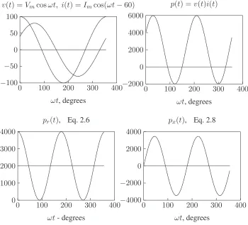
The peak amplitude Vm, and the phase angleθv of the sinusoidal supplyv(t) = Vmcos(ωt+θv). The impedance magnitudeZ, and its phase angleγ of the load. The program should produce plots fori(t),v(t),p(t),pr(t)andpx(t), similar to Example 2.1. Run the program forVm= 100V,θv = 0and the following loads: An inductive load,Z = 1.256 60◦ Ω

A capacitive load,Z = 2.06 ₋30◦ _Ω

A resistive load, Z = 2.56 0◦ Ω

(a) Frompr(t)andpx(t)plots, estimate the real and reactive power for each load. Draw a conclusion regarding the sign of reactive power for inductive and capaci-tive loads.

(b) Using phasor values of current and voltage, calculate the real and reactive power for each load and compare with the results obtained from the curves.

(c) If the above loads are all connected across the same power supply, determine the total real and reactive power taken from the supply.

The following statements are used to plot the instantaneous voltage, current, and the instantaneous terms given by(2-6) and (2-8).

Vm = input(’Enter voltage peak amplitude Vm = ’);

thetav =input(’Enter voltage phase angle in degree thetav = ’); Vm = 100; thetav = 0; % Voltage amplitude and phase angle Z = input(’Enter magnitude of the load impedance Z = ’); gama = input(’Enter load phase angle in degree gama = ’); thetai = thetav - gama; % Current phase angle in degree

(9)

6 CONTENTS

theta = (thetav - thetai)*pi/180; % Degree to radian

Im = Vm/Z; % Current amplitude

wt=0:.05:2*pi; % wt from 0 to 2*pi

v=Vm*cos(wt); % Instantaneous voltage

i=Im*cos(wt + thetai*pi/180); % Instantaneous current

p=v.*i; % Instantaneous power

V=Vm/sqrt(2); I=Im/sqrt(2); % RMS voltage and current pr = V*I*cos(theta)*(1 + cos(2*wt)); % Eq. (2.6)

px = V*I*sin(theta)*sin(2*wt); % Eq. (2.8)

disp(’(a) Estimate from the plots’)

P = max(pr)/2, Q = V*I*sin(theta)*sin(2*pi/4)

P = P*ones(1, length(wt)); % Average power for plot xline = zeros(1, length(wt)); % generates a zero vector

wt=180/pi*wt; % converting radian to degree

subplot(221), plot(wt, v, wt, i,wt, xline), grid

title([’v(t)=Vm coswt, i(t)=Im cos(wt +’,num2str(thetai),’)’]) xlabel(’wt, degrees’)

subplot(222), plot(wt, p, wt, xline), grid title(’p(t)=v(t) i(t)’), xlabel(’wt, degrees’) subplot(223), plot(wt, pr, wt, P, wt,xline), grid title(’pr(t) Eq. 2.6’), xlabel(’wt, degrees’) subplot(224), plot(wt, px, wt, xline), grid title(’px(t) Eq. 2.8’), xlabel(’wt, degrees’) subplot(111)

disp(’(b) From P and Q formulas using phasor values ’)

P=V*I*cos(theta) % Average power

Q = V*I*sin(theta) % Reactive power

The result for the inductive loadZ = 1.256 60◦Ωis Enter voltage peak amplitude Vm = 100

Enter voltage phase angle in degree thatav = 0 Enter magnitude of the load impedance Z = 1.25 Enter load phase angle in degree gama = 60

(a) Estimate from the plots

P =

2000 Q =

3464

(b) For the inductive loadZ = 1.256 60◦_Ω_{, the rms values of voltage and current}

are

V = 1006 0◦

(10)

−100

−50 0 50 100

0 100 200 300 400

ωt, degrees

v(t) =Vmcosωt, i(t) =Imcos(ωt−60)

.

... .

...

. .

...

−2000 0 2000 4000 6000

0 100 200 300 400

ωt, degrees p(t) =v(t)i(t)

... .

.

...

0 1000 2000 3000 4000

0 100 200 300 400

ωt- degrees pr(t), Eq. 2.6

... ...

−4000

−2000 0 2000 4000

0 100 200 300 400

ωt, degrees px(t), Eq. 2.8

.

... .

. . . . .

...

FIGURE 3

Instantaneous current, voltage, power, Eqs. 2.6 and 2.8.

I = 70.716 0◦

1.256 60◦ = 56.576 −60◦ A

Using (2.7) and (2.9), we have

P = (70.71)(56.57) cos(60) = 2000 W Q= (70.71)(56.57) sin(60) = 3464 Var

Running the above program for the capacitive loadZ = 2.06 ₋30◦ _Ω_{will result in}

(a) Estimate from the plots

P =

2165 Q =

(11)

8 CONTENTS

Similarly, forZ = 2.56 0◦ _Ω_{, we get}

P =

2000 Q =

0

(c) With the above three loads connected in parallel across the supply, the total real and reactive powers are

P = 2000 + 2165 + 2000 = 6165 W Q= 3464₋1250 + 0 = 2214 Var

2.2.A single-phase load is supplied with a sinusoidal voltage v(t) = 200 cos(377t)

The resulting instantaneous power is

p(t) = 800 + 1000 cos(754t₋36.87◦)

(a) Find the complex power supplied to the load.

(b) Find the instantaneous currenti(t)and the rms value of the current supplied to the load.

(c) Find the load impedance.

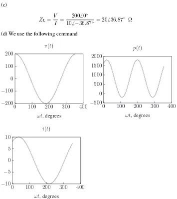
(d) UseMATLABto plotv(t),p(t), andi(t) =p(t)/v(t)over a range of0to16.67

ms in steps of 0.1 ms. From the current plot, estimate the peak amplitude, phase angle and the angular frequency of the current, and verify the results obtained in part (b). Note inMATLABthe command for array or element-by-element division is./.

p(t) = 800 + 1000 cos(754t₋36.87◦)

= 800 + 1000 cos 36.87◦cos 754t+ sin 36.87◦sin 754t

= 800 + 800 cos 754t+ 600 sin 754t

= 800[1 + cos 2(377)t] + 600 sin 2(377)t

p(t)is in the same form as (2.5), thusP = 600W, andQ= 600, Var, or S= 800 +j600 = 10006 36.87◦ VA

(b) UsingS = 1₂VmIm∗, we have

10006 36.87◦ = 1

(12)

or

Im= 106 −36.87◦ A Therefore, the instantaneous current is

i(t) = 10cos(377t₋36.87◦) A (c)

ZL= V

I =

2006 0◦

106 ₋36.87◦ = 206 36.87◦ Ω

(d) We use the following command

−200

−100 0 100 200

0 100 200 300 400

ωt, degrees v(t)

...

−500 0 500 1000 1500 2000

0 100 200 300 400

ωt, degrees p(t)

.

...

−10

−5 0 5 10

0 100 200 300 400

ωt, degrees i(t)

...

FIGURE 4

(13)

10 CONTENTS

Vm = 200;

t=0:.0001:0.01667; % wt from 0 to 2*pi

v=Vm*cos(377*t); % Instantaneous voltage

p = 800 + 1000*cos(754*t - 36.87*pi/180);% Instantaneous power

i=p./v; % Instantaneous current

wt=180/pi*377*t; % converting radian to degree xline = zeros(1, length(wt)); % generates a zero vector subplot(221), plot(wt, v, wt, xline), grid

xlabel(’wt, degrees’), title(’v(t)’) subplot(222), plot(wt, p, wt, xline), grid xlabel(’wt, degrees’), title(’p(t)’) subplot(223), plot(wt, i, wt, xline), grid

xlabel(’wt, degrees’), title(’i(t)’), subplot(111)

The result is shown in Figure 4. The inspection of current plot shows that the peak amplitude of the current is10 A, lagging voltage by36.87◦, with an angular fre-quency of 377 Rad/sec.

2.3.An inductive load consisting ofRandXin series feeding from a 2400-V rms supply absorbs 288 kW at a lagging power factor of 0.8. DetermineRandX.

... ...

. . . ... . .

V I

R X

+◦ ₋◦

FIGURE 5

An inductive load, withR_andX_{in series.}

θ= cos−10.8 = 36.87◦

The complex power is S= 288

0.86 36.87

◦ _{= 360}₆ ₃₆_.₈₇◦ _kVA

The current given fromS=V I∗, is

I = 360×10

3₆ ₋₃₆_.₈₇◦

24006 0◦ = 1506 −36.87 A

Therefore, the series impedance is

Z =R+jX = V

I =

24006 0◦

1506 ₋36.87◦ = 12.8 +j9.6 Ω

(14)

2.4.An inductive load consisting ofR andX in parallel feeding from a 2400-V rms supply absorbs 288 kW at a lagging power factor of 0.8. DetermineRandX.

.

An inductive load, withR_andX_{in parallel.}

The complex power is

S = 288

2.5.Two loads connected in parallel are supplied from a single-phase 240-V rms source. The two loads draw a total real power of 400 kW at a power factor of 0.8 lagging. One of the loads draws 120 kW at a power factor of 0.96 leading. Find the complex power of the other load.

θ= cos−10.8 = 36.87◦

The total complex load is

S = 400

0.86 36.87◦= 5006 36.87◦ kVA = 400kW+j300kvar The120kW load complex power is

S= 120

0.966 −16.26

(15)

12 CONTENTS

Therefore, the second load complex power is

S2= 400 +j300−(120−j35) = 280kW+j335kvar

2.6.The load shown in Figure 7 consists of a resistanceRin parallel with a capac-itor of reactanceX. The load is fed from a single-phase supply through a line of impedance8.4 +j11.2 Ω. The rms voltage at the load terminal is12006 0◦ V rms, and the load is taking 30 kVA at 0.8 power factor leading.

(a) Find the values ofRandX. (b) Determine the supply voltageV.

✖✕ ✗✔ .

... ... ...

. . . ... . . .

V

I

8.4 +j11.2 Ω

R −jX

12006 0◦V +

−

FIGURE 7

Circuit for Problem 2.6.

θ= cos−10.8 = 36.87◦

The complex power is

S = 306 ₋36.87◦ = 24kW₋j18kvar (a)

R= |V|

2

P =

(1200)2

24000 = 60 Ω

X= |V|

2

Q =

(1200)2

18000 = 80 Ω

FromS=V I∗_{, the current is}

I = 300006 36.87◦

12006 0◦ = 256 36.87 A

Thus, the supply voltage is

(16)

2.7.Two impedances,Z1 = 0.8 +j5.6 Ω andZ2 = 8−j16 Ω, and a single-phase motor are connected in parallel across a 200-V rms, 60-Hz supply as shown in Figure 8. The motor draws 5 kVA at 0.8 power factor lagging.

.

(a) Find the complex powersS1,S2for the two impedances, andS3for the motor. (b) Determine the total power taken from the supply, the supply current, and the overall power factor.

(c) A capacitor is connected in parallel with the loads. Find the kvar and the ca-pacitance inµF to improve the overall power factor to unity. What is the new line current?

(a) The load complex power are

S1 = |

Therefore, the total complex power is

St= 6 +j8 = 106 53.13◦kVA (b) FromS=V I∗, the current is

I = 100006 −53.13◦

2006 0◦ = 506 −53.13 A

(17)

14 CONTENTS

(c) For overall unity power factor,QC = 8000Var, and the capacitive impedance is

ZC = | V_|2 SC∗

= (200)

2

j8000 =−j5 Ω

and the capacitance is

C= 10

6

(2π)(60)(5) = 530.5 µF

The new current is

I = 60006 0◦

2006 0◦ = 306 0 A

2.8.Two single-phase ideal voltage sources are connected by a line of impedance of

0.7 +j2.4 Ωas shown in Figure 9.V1= 5006 16.26◦V andV2= 5856 0◦V. Find the complex power for each machine and determine whether they are delivering or receiving real and reactive power. Also, find the real and the reactive power loss in the line.

✖✕ ✗✔ .

...

✖✕ ✗✔ ...

. . . ... .

5006 16.26◦_V

I12

0.7 +j2.4 Ω

5856 0◦_V +

−

+

−

FIGURE 9

I12=

5006 16.26◦₋5856 0◦

0.7 +j2.4 = 42 +j56 = 706 53.13 ◦ _A

S12=V1I12∗ = (5006 16.26◦)(706 −53.13◦) = 350006 −36.87◦

= 28000₋j21000 VA S21=V2I21∗ = (5856 0◦)(−706 −53.13◦) = 409506 −53.13◦

(18)

From the above results, sinceP1is positive andP2 is negative, source 1 generates

28kW, and source 2 receives24.57kW, and the real power loss is3.43kW. Sim-ilarly, sinceQ1 is negative, source 1 receives21kvar and source 2 delivers32.76 kvar. The reactive power loss in the line is11.76kvar.

2.9.Write aMATLABprogram for the system of Example 2.5 such that the voltage magnitude of source 1 is changed from 75 percent to 100 percent of the given value in steps of 1 volt. The voltage magnitude of source 2 and the phase angles of the two sources is to be kept constant. Compute the complex power for each source and the line loss. Tabulate the reactive powers and plotQ1,Q2, andQLversus voltage magnitude_|V1|. From the results, show that the flow of reactive power along the interconnection is determined by the magnitude difference of the terminal voltages. We use the following commands

E1 = input(’Source # 1 Voltage Mag. = ’); a1 = input(’Source # 1 Phase Angle = ’); E2 = input(’Source # 2 Voltage Mag. = ’); a2 = input(’Source # 2 Phase Angle = ’); R = input(’Line Resistance = ’);

X = input(’Line Reactance = ’);

Z = R + j*X; % Line impedance

E1 = (0.75*E1:1:E1)’; % Change E1 form 75% to 100% E1 a1r = a1*pi/180; % Convert degree to radian k = length(E1);

E2 = ones(k,1)*E2;%create col. Array of same length for E2 a2r = a2*pi/180; % Convert degree to radian V1=E1.*cos(a1r) + j*E1.*sin(a1r);

V2=E2.*cos(a2r) + j*E2.*sin(a2r); I12 = (V1 - V2)./Z; I21=-I12;

S1= V1.*conj(I12); P1 = real(S1); Q1 = imag(S1); S2= V2.*conj(I21); P2 = real(S2); Q2 = imag(S2); SL= S1+S2; PL = real(SL); QL = imag(SL); Result1=[E1, Q1, Q2, QL];

disp(’ E1 Q-1 Q-2 Q-L ’)

disp(Result1)

plot(E1, Q1, E1, Q2, E1, QL), grid xlabel(’ Source #1 Voltage Magnitude’) ylabel(’ Q, var’)

text(112.5, -180, ’Q2’)

text(112.5, 5,’QL’), text(112.5, 197, ’Q1’)

(19)

16 CONTENTS

Source # 1 Voltage Mag. = 120 Source # 1 Phase Angle = -5 Source # 2 Voltage Mag. = 100 Source # 2 Phase Angle = 0 Line Resistance = 1

Line Reactance = 7

E1 Q-1 Q-2 Q-L

90.0000 -105.5173 129.1066 23.5894 91.0000 -93.9497 114.9856 21.0359 92.0000 -82.1021 100.8646 18.7625 93.0000 -69.9745 86.7435 16.7690 94.0000 -57.5669 72.6225 15.0556 95.0000 -44.8794 58.5015 13.6221 96.0000 -31.9118 44.3804 12.4687 97.0000 -18.6642 30.2594 11.5952 98.0000 -5.1366 16.1383 11.0017 99.0000 8.6710 2.0173 10.6883 100.0000 22.7586 -12.1037 10.6548 101.0000 37.1262 -26.2248 10.9014 102.0000 51.7737 -40.3458 11.4279 103.0000 66.7013 -54.4668 12.2345 104.0000 81.9089 -68.5879 13.3210 105.0000 97.3965 -82.7089 14.6876 106.0000 113.1641 -96.8299 16.3341 107.0000 129.2117 -110.9510 18.2607 108.0000 145.5393 -125.0720 20.4672 109.0000 162.1468 -139.1931 22.9538 110.0000 179.0344 -153.3141 25.7203 111.0000 196.2020 -167.4351 28.7669 112.0000 213.6496 -181.5562 32.0934 113.0000 231.3772 -195.6772 35.7000 114.0000 249.3848 -209.7982 39.5865 115.0000 267.6724 -223.9193 43.7531 116.0000 286.2399 -238.0403 48.1996 117.0000 305.0875 -252.1614 52.9262 118.0000 324.2151 -266.2824 57.9327 119.0000 343.6227 -280.4034 63.2193 120.0000 363.3103 -294.5245 68.7858

(20)

−300

Source # 1 Voltage magnitude .

Reactive power versus voltage magnitude.

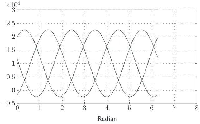
2.10.A balanced three-phase source with the following instantaneous phase volt-ages

van = 2500 cos(ωt)

vbn= 2500 cos(ωt−120◦) vcn= 2500 cos(ωt−240◦)

supplies a balanced Y-connected load of impedanceZ = 2506 36.87◦ _Ω_{per phase.}

(a) UsingMATLAB, plot the instantaneous powerspa,pb,pcand their sum versus ωtover a range of0 : 0.05 : 2π on the same graph. Comment on the nature of the instantaneous power in each phase and the total three-phase real power.

(b) Use (2.44) to verify the total power obtained in part (a). We use the following commands

wt=0:.02:2*pi;

pa=25000*cos(wt).*cos(wt-36.87*pi/180);

(21)

18 CONTENTS

plot(wt, pa, wt, pb, wt, pc, wt, p), grid xlabel(’Radian’)

disp(’(b)’)

V = 2500/sqrt(2); gama = acos(0.8);

Z = 250*(cos(gama)+j*sin(gama)); I = V/Z;

P = 3*V*abs(I)*0.8

−0.5

Instantaneous powers and their sum for Problem 2.10.

(b)

2.11.A 4157-V rms phase supply is applied to a balanced Y-connected three-phase load consisting of three identical impedances of 486 36.87◦ Ω. Taking the phase to neutral voltageVanas reference, calculate

(a) The phasor currents in each line.

(b) The total active and reactive power supplied to the load. Van =

4157 √

(22)

WithVanas reference, the phase voltages are:

Van= 24006 0◦ V Vbn= 24006 −120◦ V Van= 24006 −240◦V (a) The phasor currents are:

Ia= Van

Z =

24006 0◦

486 36.87◦ = 506 −36.87◦ A

Ib = Vbn

Z =

24006 ₋120◦

486 36.87◦ = 506 −156.87◦ A

Ic= Vcn

Z =

24006 ₋240◦

486 36.87◦ = 506 −276.87◦ A

(b) The total complex power is

S = 3VanIa∗= (3)(24006 0◦)(506 36.87◦) = 3606 36.87◦kVA

= 288kW+j216KVAR

2.12.Repeat Problem 2.11 with the same three-phase impedances arranged in a∆

connection. TakeVabas reference.

Van =

4157 √

3 = 2400 V

WithVabas reference, the phase voltages are:

Iab= Vab

Z =

41576 0◦

486 36.87◦ = 86.66 −36.87◦ A

Ia=

√

36 ₋30◦Iab= (

√

36 ₋30◦)(86.66 ₋36.87◦= 1506 ₋66.87◦ A For positive phase sequence, current in other lines are

Ib = 1506 −186.87◦ A, andIc= 1506 53.13◦ A (b) The total complex power is

S= 3VabIab∗ = (3)(41576 0◦)(86.66 36.87◦) = 10806 36.87◦ kVA

= 864kW+j648kvar

(23)

20 CONTENTS

(a) Current in phasea.

(b) Total complex power supplied from the source.

(c) Magnitude of the line-to-line voltage at the load terminal.

Van = 207√.85

3 = 120 V

Transforming the delta connected load to an equivalent Y-connected load, result in the phase ’a’ equivalent circuit, shown in Figure 13.

...

The per phase equivalent circuit for Problem 2.13.

(a)

Ia=

1206 0◦

6 +j8 = 126 −53.13 ◦ _A

(b) The total complex power is

S = 3VanIa∗ = (3)(1206 0◦)(126 53.13◦= 43206 53.13◦ VA

= 2592W+j3456Var (c)

(24)

Thus, the magnitude of the line-to-line voltage at the load terminal isVL=√3(93.72) =

162.3V.

2.14.Three parallel three-phase loads are supplied from a 207.85-V rms, 60-Hz three-phase supply. The loads are as follows:

Load 1: A 15 HP motor operating at full-load, 93.25 percent efficiency, and 0.6 lagging power factor.

Load 2: A balanced resistive load that draws a total of 6 kW.

Load 3: A Y-connected capacitor bank with a total rating of 16 kvar.

(a) What is the total system kW, kvar, power factor, and the supply current per phase?

(b) What is the system power factor and the supply current per phase when the resistive load and induction motor are operating but the capacitor bank is switched off?

The real power input to the motor is

P1= (15)(746)

0.9325 = 12 kW

S1= 12

0.66 53.13

◦ _kVA_{= 12}_kW₊_j₁₆_kvar

S2= 6kW+j0kvar S3= 0kW−j16kvar (a) The total complex power is

S = 186 0◦ kVA= 18kW+j0kvar The supply current is

I = 18000

(3)(120) = 506 0◦ A, at unity power factor

(b) With the capacitor switched off, the total power is S = 18 +j16 = 24.086 41.63◦ kVA

I = 240836 −41.63

(3)(1206 0◦₎ = 66.896 −41.63◦ A

(25)

22 CONTENTS

2.15.Three loads are connected in parallel across a 12.47 kV three-phase supply. Load 1: Inductive load, 60 kW and 660 kvar.

Load 2: Capacitive load, 240 kW at 0.8 power factor. Load 3: Resistive load of 60 kW.

(a) Find the total complex power, power factor, and the supply current.

(b) A Y-connected capacitor bank is connected in parallel with the loads. Find the total kvar and the capacitance per phase inµF to improve the overall power factor to 0.8 lagging. What is the new line current?

S1 = 60kW+j660kvar S2 = 240kW−j180kvar S3 = 60kW+ j0kvar (a) The total complex power is

S = 360kW+j480kvar= 6006 53.13◦kVA The phase voltage is

V = 12√.47

3 = 7.26 0 ◦ _kV

The supply current is

I = 6006 −53.13◦

(3)(7.2) = 27.776 −53.13 ◦ _A

The power factor iscos 53.13◦ = 0.6lagging.

(b) The net reactive power for0.8power factor lagging is Q′ = 360 tan 36.87◦ = 270 kvar

Therefore, the capacitor kvar isQc= 480−270 = 210kvar, orSc=−j210kVA.

Xc= | VL|2

S_c∗ =

(12.47_×1000)2

j210000 =−j740.48 Ω

C= 10

6

(26)

...

The power diagram for Problem 2.15.

I = S∗

V∗ =

360₋j270

(3)(7.2) = 20.8356 −36.87 ◦ _A

2.16.A balanced ∆-connected load consisting of a pure resistances of18 Ωper phase is in parallel with a purely resistive balanced Y-connected load of 12 Ω

per phase as shown in Figure 15. The combination is connected to a three-phase balanced supply of 346.41-V rms (line-to-line) via a three-phase line having an inductive reactance ofj3 Ωper phase. Taking the phase voltageVan as reference, determine

(a) The current, real power, and reactive power drawn from the supply.

(b) The line-to-neutral and the line-to-line voltage of phaseaat the combined load terminals.

(27)

24 CONTENTS

Transforming the delta connected load to an equivalent Y-connected load, result in the phase ’a’ equivalent circuit, shown in Figure 16.

...

. . . . . . . . . . . . . . . . . . . . . . . . . . . . . . . . . . . . . . . . . . . . . . . . . . . . . . . . . ... . . . ... . . . ...

... j3 Ω

6 Ω 12 Ω

V1 = 2006 0◦V V2 +

−

❜

❜ a

n

...

. . . . . . . . . . . . . . . . . . . . . . . . . . . . . . . . . . . . . .

... ... . . . . ... I

I1 I2

FIGURE 16

(a)

Van =

346.41 √

3 = 200 V

The input impedance is

Z = (12)(6)

12 + 6 +j3 = 4 +j3 Ω

Ia=

2006 0◦

4 +j3 = 406 −36.87 ◦ _A

The total complex power is

S= 3VanIa∗ = (3)(2006 0◦)(406 36.87◦) = 240006 36.87◦ VA

= 19200W+j14400Var (b)

V2 = 2006 0◦−(j3)(406 −36.87◦) = 1606 −36.87◦ A

Thus, the magnitude of the line-to-line voltage at the load terminal isVL=√3(160) =

(28)

3.1.A three-phase, 318.75-kVA, 2300-V alternator has an armature resistance of 0.35Ω/phase and a synchronous reactance of 1.2Ω/phase. Determine the no-load line-to-line generated voltage and the voltage regulation at

(a) Full-load kVA, 0.8 power factor lagging, and rated voltage. (b) Full-load kVA, 0.6 power factor leading, and rated voltage.

Vφ=

2300 √

3 = 1327.9 V

(a) For318.75kVA,0.8power factor lagging,S = 3187506 36.87◦VA.

Ia= S

∗

3V∗

φ

= 3187506 −36.87◦

(3)(1327.9) = 806 −36.87 ◦ _A

Eφ= 1327.9 + (0.35 +j1.2)(806 −36.87◦) = 1409.26 2.44◦ V The magnitude of the no-load generated voltage is

ELL =√3 1409.2 = 2440.8V, and the voltage regulation is

V.R.= 2440.8−2300

2300 ×100 = 6.12%

(b) For318.75kVA,0.6power factor leading,S = 3187506 ₋53.13◦VA.

Ia= S

∗

3V∗

φ

= 3187506 53.13◦

(3)(1327.9 = 806 53.13 ◦ _A

(29)

26 CONTENTS

Eφ= 1327.9 + (0.35 +j1.2)(806 53.13◦) = 1270.46 3.61◦ V The magnitude of the no-load generated voltage is

ELL =√3 1270.4 = 2220.4V, and the voltage regulation is

V.R.= 2200.4−2300

2300 ×100 =−4.33%

3.2.A 60-MVA, 69.3-kV, three-phase synchronous generator has a synchronous reactance of 15Ω/phase and negligible armature resistance.

(a) The generator is delivering rated power at 0.8 power factor lagging at the rated terminal voltage to an infinite bus bar. Determine the magnitude of the generated emf per phase and the power angleδ.

(b) If the generated emf is 36 kV per phase, what is the maximum three-phase power that the generator can deliver before losing its synchronism?

(c) The generator is delivering 48 MW to the bus bar at the rated voltage with its field current adjusted for a generated emf of 46 kV per phase. Determine the armature current and the power factor. State whether power factor is lagging or leading?

Vφ=

69.3 √

3 = 40 kV

(a) For60kVA,0.8power factor lagging,S = 600006 36.87◦kVA.

Ia= S∗

3V∗

φ

= 600006 −36.87◦

(3)(40) = 5006 −36.87◦ A

Eφ= 40 + (j15)(5006 −36.87◦)×10−3 = 44.96 7.675◦ kV (b)

Pmax =

3_|E_||V_| Xs

= (3)(36)(40)

15 = 288 MW

(c) ForP = 48MW, andE = 46KV/phase, the power angle is given by

(30)

or

δ= 7.4947◦

and solving for the armature current fromE=V +jXsIa, we have

Ia=

460006 7.4947◦₋₄₀₀₀₀₆ ₀◦

j15 = 547.476 −43.06 ◦ _A

The power factor iscos−1₄₃_._{06 = 0}_.₇₃₀₆_lagging.

3.3.A 24,000-kVA, 17.32-kV, Y-connected synchronous generator has a synchronous reactance of 5Ω/phase and negligible armature resistance.

(a) At a certain excitation, the generator delivers rated load, 0.8 power factor lag-ging to an infinite bus bar at a line-to-line voltage of 17.32 kV. Determine the excitation voltage per phase.

(b) The excitation voltage is maintained at 13.4 KV/phase and the terminal voltage at 10 KV/phase. What is the maximum three-phase real power that the generator can develop before pulling out of synchronism?

(c) Determine the armature current for the condition of part (b).

Vφ=

17.32 √

3 = 10 kV

(a) For24000kVA,0.8power factor lagging,S= 240006 36.87◦ kVA.

Ia= S

∗

3V∗

φ

= 240006 −36.87◦

(3)(10) = 8006 −36.87 ◦ _A

Eφ= 10 + (j5)(8006 −36.87◦)×10−3 = 12.8066 14.47◦ kV (b)

Pmax=

3_|E_||V_| Xs

= (3)(13.4)(10)

5 = 80.4 MW

(c) At maximum power transferδ= 90◦, and solving for the armature current from E =V +jXsIa, we have

Ia=

134006 90◦₋100006 0◦

(31)

28 CONTENTS

The power factor iscos−1₃₆_._{73 = 0}_.₇₃₀₆_leading.

3.4.A 34.64-kV, 60-MVA, three-phase salient-pole synchronous generator has a direct axis reactance of 13.5Ω and a quadrature-axis reactance of 9.333Ω. The armature resistance is negligible.

(a) Referring to the phasor diagram of a salient-pole generator shown in Figure 17, show that the power angleδis given by

δ = tan−1

Ã

Xq|Ia|cosθ V +Xq|Ia|sinθ

!

(b) Compute the load angle δ and the per phase excitation voltage E when the generator delivers rated MVA, 0.8 power factor lagging to an infinite bus bar of 34.64-kV line-to-line voltage.

(c) The generator excitation voltage is kept constant at the value found in part (b). UseMATLABto obtain a plot of the power angle curve, i.e., equation (3.26) over a range ofd= 0 :.05 : 180◦_{. Use the command [P}_max_{, k] = max(P);}_d_max₌_d₍_k₎_,

to obtain the steady-state maximum powerPmaxand the corresponding power an-gledmax.

Phasor diagram of a salient-pole generator for Problem 3.4.

(a) Form the phasor diagram shown in Figure 17, we have

(32)

or

δ = tan−1 Xq|Ia|cosθ

V +Xq|Ia|sinθ (b)

Vφ=

34.64 √

3 = 20 kV

(a) For60MVA,0.8power factor lagging,S = 606 36.87◦MVA

Ia= S∗

3V∗

φ

= 600006 −36.87◦

(3)(20) = 10006 −36.87 ◦ _A

δ= tan−1 (9.333)(1000)(0.8)

20000 + (9.333)(1000)(0.6) = 16.26 ◦

The magnitude of the no-load generated emf per phase is given by

|E_| = _|V_|cosδ+Xd|Ia|sin(θ+δ)

= 20 cos 16.26◦+ (13.5)(1000)(10−3) sin 53.13◦ = 30 kV (c) We use the following commands

V = 20000; Xd = 13.5; Xq = 9.333; theta=acos(0.8);

Ia = 20E06/20000;

delta = atan(Xq*Ia*cos(theta)/(V + Xq*Ia*sin(theta))); deltadg=delta*180/pi;

E = V*cos(delta)+Xd*Ia*sin(theta+delta); E_KV = E/1000; % Excitaiton voltage in kV fprintf(’Power angle = %g Degree \n’, deltadg) fprintf(’E = %g kV \n\n’, E_KV)

deltadg = (0:.25:180)’; delta=deltadg*pi/180;

P=3*E*V/Xd*sin(delta)+3*V^2*(Xd-Xq)/(2*Xd*Xq)*sin(2*delta); P = P/1000000; % Power in MW

plot(deltadg, P), grid

xlabel(’Delta - Degree’), ylabel(’P - MW’) [Pmax, k]=max(P); delmax=deltadg(k);

fprintf(’Max power = %g MW’,Pmax)

(33)

30 CONTENTS

Power angle curve for Problem 3.4.

The result is

Power angle = 16.2598 Degree E = 30 kV

Max power = 138.712 MW at power angle 75 degree

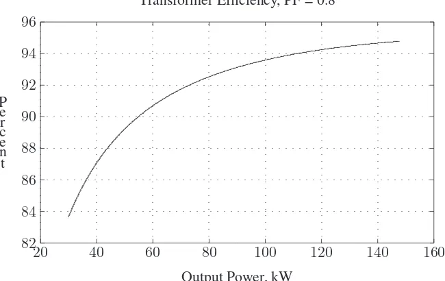
3.5.A 150-kVA, 2400/240-V single-phase transformer has the parameters as shown in Figure 19.

.

Transformer circuit for Problem 3.5.

(a) Determine the equivalent circuit referred to the high-voltage side.

(34)

(c) Find the primary voltage and voltage regulation when the transformer is oper-ating at full-load 0.8 power factor leading.

(d) Verify your answers by running thetransprogram inMATLABand obtain the transformer efficiency curve.

(a) Referring the secondary impedance to the primary side, the transformer equiv-alent impedance referred to the high voltage-side is

Ze1= 0.2 +j0.45 +

Equivalent circuit referred to the high-voltage side.

(b) At full-load 0.8 power factor laggingS = 1506 36.87◦ kVA, and the referred primary current is

I2′ = S∗ The voltage regulation is

V.R.= 2453.933−2400

2400 ×100 = 2.247%

(c) At full-load 0.8 power factor leadingS = 1506 ₋36.87◦kVA, and the referred primary current is

(35)

32 CONTENTS

The voltage regulation is

V.R.= 2453.933−2400

2400 ×100 =−0.541%

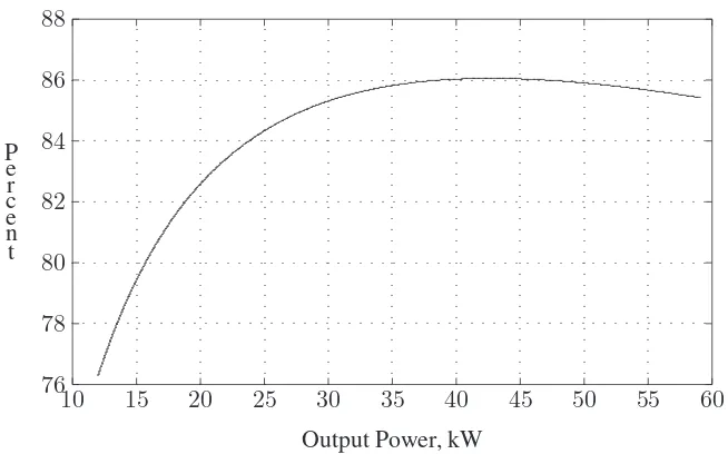
(d) Enteringtransat theMATLABprompt, result in

82

Output Power, kW Transformer Efficiency, PF = 0.8

.

Efficiency curve of Problem 3.5.

TRANSFORMER ANALYSIS

Type of parameters for input Select

---

---To obtain equivalent circuit from tests 1 To input individual winding impedances 2 To input transformer equivalent impedance 3

To quit 0

Select number of menu --> 2

Enter Transformer rated power in kVA, S = 150 Enter rated low voltage in volts = 240

(36)

Enter LV winding series impedance R1+j*X1 in ohm=0.002+j*.0045 Enter HV winding series impedance R2+j*X2 in ohm=0.2+j*0.45 Enter ’lv’ within quotes for low side shunt branch or

enter ’hv’ within quotes for high side shunt branch -> ’hv’ Shunt resistance in ohm (if neglected enter inf) = 1000 Shunt reactance in ohm (if neglected enter inf) = 1500

Shunt branch ref. to LV side Shunt branch ref. to HV side

Rc = 10.000 ohm Rc = 1000.000 ohm

Xm = 15.000 ohm Xm = 1500.000 ohm

Series branch ref. to LV side Series branch ref.to HV side Ze = 0.0040 + j 0.0090 ohm Ze = 0.4000 + j 0.90 ohm

Hit return to continue

Enter load kVA, S2 = 150

Enter load power factor, pf = 0.8

Enter ’lg’ within quotes for lagging pf or ’ld’ within quotes for leading pf -> ’lg’ Enter load terminal voltage in volt, V2 = 240 Secondary load voltage = 240.000 V

Secondary load current = 625.000 A at -36.87 degrees Current ref. to primary = 62.500 A at -36.87 degrees Primary no-load current = 2.949 A at -33.69 degrees Primary input current = 65.445 A at -36.73 degrees Primary input voltage = 2453.933 V at 0.70 degrees Voltage regulation = 2.247 percent

Transformer efficiency = 94.249 percent

Maximum efficiency is 95.238 %occurs at 288 kVA with 0.8pf

The efficiency curve is shown in Figure 21. The analysis is repeated for the full-load kVA, 0.8 power factor leading.

3.6. A 60-kVA, 4800/2400-V single-phase transformer gave the following test results:

1. Rated voltage is applied to the low voltage winding and the high voltage winding is open-circuited. Under this condition, the current into the low voltage winding is 2.4 A and the power taken from the 2400 V source is 3456 W.

2. A reduced voltage of 1250 V is applied to the high voltage winding and the low voltage winding is short-circuited. Under this condition, the current flow-ing into the high voltage windflow-ing is 12.5 A and the power taken from the 1250 V source is 4375 W.

(37)

34 CONTENTS

(b) Determine voltage regulation and efficiency when transformer is operating at full-load, 0.8 power factor lagging, and a terminal voltage of 2400 V.

(c) What is the load kVA for maximum efficiency and the maximum efficiency at 0.8 power factor?

(d) Determine the efficiency when transformer is operating at 3/4 full-load, 0.8 power factor lagging, and a terminal voltage of 2400 V.

(e) Verify your answers by running thetransprogram inMATLABand obtain the transformer efficiency curve.

(a) From the no-load test data

R_cLV = |V2|

2

P0

= (2400)

2

3456 = 1666.667 Ω

Ic= |V2| R_cLV =

2400

1666.67 = 1.44 A

Im=

q

I2

0 −Ic2 =

q

(2.4)2₋₍₁_.₄₄₎2_{= 1}_.₉₂ _A

X_mLV = |V2|

Im

= 2400

1.92 = 1250 Ω

The shunt parameters referred to the high-voltage side are

R_{C HV} =

µ₄₈₀₀

2400

¶2

1666.667 = 6666.667 Ω

X_mHV =

µ₄₈₀₀

2400

¶2

1250 = 5000 Ω

From the short-circuit test data Ze1 = Vsc

Isc

= 1250

12.5 = 100 Ω

Re1 = Psc

(Isc)2

= 4375

(38)

Xe1=

q

Z2

e1−R2e1 =

q

(100)2₋₍₂₈₎2_{= 96 Ω}

(b) At full-load 0.8 power factor laggingS = 606 36.87◦ kVA, and the referred primary current is

I2

′ = S∗

V∗ =

600006 ₋36.87◦

4800 = 12.56 −36.87 ◦ _A

V1= 4800 + (28 +j96)(12.56 −36.87◦) = 5848.296 7.368◦ V The voltage regulation is

V.R.= 5848.29−4800

4800 ×100 = 21.839%

Efficiency at full-load, 0.8 power factor is

η = (60)(0.8)

(60)(0.8) + 3.456 + 4.375×100 = 85.974 %

(c) At Maximum efficiencyPc=Pcu, and we have Pcu ∝ Sf l2

Pc ∝ Smaxη2 Therefore, the load kVA at maximum efficiency is

Smaxη =

s

Pc Pcu

Sf l=

r

3456

4375 60 = 53.327 kVA

and the maximum efficiency at 0.8 power factor is

η= (53.327)(0.8)

(53.327)(0.8) + 3.456 + 3.456×100 = 86.057 %

(d) At3/4full-load, the copper loss is

Pcu3/4 = (3/4)2(4375) = 2460.9375 W Therefore, the efficiency at3/4full-load, 0.8 power factor is

η = (45)(0.8)

(45)(0.8) + 3.456 + 2.4609×100 = 85.884 %

(39)

36 CONTENTS

TRANSFORMER ANALYSIS

Type of parameters for input Select

---

---To obtain equivalent circuit from tests 1 To input individual winding impedances 2 To input transformer equivalent impedance 3

To quit 0

Select number of menu --> 1

Enter Transformer rated power in kVA, S = 60 Enter rated low voltage in volts = 2400 Enter rated high voltage in volts = 4800

Open circuit test data

---Enter ’lv’ within quotes for data referred to low side or enter ’hv’ within quotes for data referred to high side ->’lv’ Enter input voltage in volts, Vo = 2400

Enter no-load current in Amp, Io = 2.4

Enter no-load input power in Watt, Po = 3456

Short circuit test data

---Enter ’lv’ within quotes for data referred to low side or enter ’hv’ within quotes for data referred to high side ->’hv’ Enter reduced input voltage in volts, Vsc = 1250

Enter input current in Amp, Isc = 12.5 Enter input power in Watt, Psc = 4375

Shunt branch ref. to LV side Shunt branch ref. to HV side

Rc = 1666.667 ohm Rc = 6666.667 ohm

Xm = 1250.000 ohm Xm = 5000.000 ohm

Series branch ref. to LV side Series branch ref.to HV side Ze = 7.0000 + j 24.0000 ohm Ze = 28.000 + j 96.000 ohm Hit return to continue

Enter load KVA, S2 = 60

Enter load power factor, pf = 0.8

Enter ’lg’ within quotes for lagging pf or ’ld’ within quotes for leading pf -> ’lg’ Enter load terminal voltage in volt, V2 = 2400 Secondary load voltage = 2400.000 V

(40)

Current ref. to primary = 12.500 A at -36.87 degrees Primary no-load current = 1.462 A at -53.13 degrees Primary input current = 13.910 A at -38.56 degrees Primary input voltage = 5848.290 V at 7.37 degrees Voltage regulation = 21.839 percent

Transformer efficiency = 85.974 percent

Maximum efficiency is 86.057%occurs at 53.33kVA with 0.8pf

The efficiency curve is shown in Figure 22. The analysis is repeated for the3/4

full-load kVA, 0.8 power factor lagging.

76

Output Power, kW Transformer Efficiency, PF = 0.8

.

Efficiency curve of Problem 3.6.

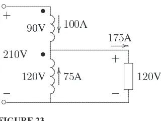
3.7.A two-winding transformer rated at 9-kVA, 120/90-V, 60-HZ has a core loss of 200 W and a full-load copper loss of 500 W.

(a) The above transformer is to be connected as an auto transformer to supply a load at 120 V from 210 V source. What kVA load can be supplied without exceed-ing the current ratexceed-ing of the windexceed-ings? (For this part assume an ideal transformer.) (b) Find the efficiency with the kVA loading of part (a) and 0.8 power factor. The two-winding transformer rated currents are:

ILV =

9000

(41)

38 CONTENTS

IHV = 9000

120 = 75 A

The auto transformer connection is as shown in Figure 23.

...

Auto transformer connection for Problem 3.7.

(a) With windings carrying rated currents, the auto transformer rating is S= (120)(175)(10−3) = 21 kVA

(b) Since the windings are subjected to the same rated voltages and currents as the two-winding transformer, the auto transformer copper loss and the core loss at the rated values are the same as the two-winding transformer. Therefore, the auto transformer efficiency at0.8power factor is

η = (21000)(0.8)

(21000)(0.8) + 200 + 500×100 = 96 %

3.8.Three identical 9-MVA, 7.2-kV/4.16-kV, single-phase transformers are con-nected in Y on the high-voltage side and∆on the low voltage side. The equiv-alent series impedance of each transformer referred to the high-voltage side is

0.12 +j0.82 Ωper phase. The transformer supplies a balanced three-phase load of 18 MVA, 0.8 power factor lagging at 4.16 kV. Determine the line-to-line voltage at the high-voltage terminals of the transformer.

The per phase equivalent circuit is shown in Figure 24. The load complex power is S= 180006 36.87◦ kVA

I1 =

180006 ₋36.87◦

(42)

.

...

.

... ... Ze1 = 0.12 +j0.82

V1 V′

2 = 7200V I1

. ...

. . +

−

❜

FIGURE 24

The per phase equivalent circuit of Problem 3.8.

V1= 7.26 0◦+ (0.12 +j0.82)(833.3336 −36.87◦)(10−3) = 7.70546 3.62◦ kV

Therefore, the magnitude of the primary line-to-line supply voltage is V1LL =

√

3(7.7054) = 13.346kV.

3.9.A 400-MVA, 240-kV/24-KV, three-phase Y-∆transformer has an equivalent series impedance of 1.2 +j6 Ωper phase referred to the high-voltage side. The transformer is supplying a three-phase load of 400-MVA, 0.8 power factor lagging at a terminal voltage of 24 kV (line to line) on its low-voltage side. The primary is supplied from a feeder with an impedance of0.6 +j1.2 Ω per phase. Deter-mine the line-to-line voltage at the high-voltage terminals of the transformer and the sending-end of the feeder.

The per phase equivalent circuit referred to the primary is is shown in Figure 25. The load complex power is

.

... ...

.

...

◦

◦... +

−

V1 . .

... Zf = 0.6 +j1.2 Ze1 = 1.2 +j6

Vs V2′ = 138.564kV

I1 . ...

. . . +

−

❜

FIGURE 25

(43)

40 CONTENTS

and the referred secondary voltage per phase is

V₂′ = 240_√

3 = 138.564 kV

I1=

4000006 ₋36.87◦

(3)(138.564) = 962.256 −36.87◦ A

V1= 138.5646 0◦+ (1.2 +j6)(962.256 −36.87◦)(10−3) = 1436 1.57◦ kV Therefore, the line-to-line voltage magnitude at the high voltage terminal of the transformer isV1LL =

√

3(143) = 247.69kV.

Vs= 138.5646 0◦+ (1.8 +j7.2)(962.256 −36.87◦)(10−3) = 144.1776 1.79◦kV Therefore, the line-to-line voltage magnitude at the sending end of the feeder is V1LL=

√

3(143) = 249.72kV.

3.10.In Problem 3.9, with transformer rated values as base quantities, express all impedances in per unit. Working with per-unit values, determine the line-to-line voltage at the high-voltage terminals of the transformer and the sending-end of the feeder.

With the transformer rated MVA as base, the HV-side base impedance is

ZB=

(240)2

400 = 144 Ω

The transformer and the feeder impedances in per unit are

Ze =

(1.2 +j6)

144 = 0.008333 +j0.04166pu

Zf =

(0.6 +j1.2)

144 = 0.004166 +j0.00833pu

I = 16 −36.87◦

16 0◦ = 16 −36.87◦pu

(44)

Therefore, the line-to-line voltage magnitude at the high-voltage terminal of the transformer is(1.03205)(240) = 247.69kV

Vs= 1.06 0◦+ (0.0125 +j0.05)(16 −36.87◦ = 1.04056 1.79◦ pu

Therefore, the line-to-line voltage magnitude at the high voltage terminal of the transformer is(1.0405)(240) = 249.72kV

3.11.A three-phase, Y-connected, 75-MVA, 27-kV synchronous generator has a synchronous reactance of9.0 Ωper phase. Using rated MVA and voltage as base values, determine the per unit reactance. Then refer this per unit value to a 100-MVA, 30-kV base.

The base impedance is

ZB = (KVB) 2

M V AB

= (27)

2

75 = 9.72 Ω

Xpu=

9

9.72 = 0.926 pu

The generator reactance on a 100-MVA, 30-kV base is

X_punew = 0.926

µ₁₀₀

75

¶ µ₂₇

30

¶2

= 1.0 pu

3.12.A 40-MVA, 20-kV/400-kV, single-phase transformer has the following series impedances:

Z1 = 0.9 +j1.8 Ω and Z2= 128 +j288 Ω

Using the transformer rating as base, determine the per unit impedance of the trans-former from the ohmic value referred to the low-voltage side. Compute the per unit impedance using the ohmic value referred to the high-voltage side.

The transformer equivalent impedance referred to the low-voltage side is

Ze1= 0.9 +j1.8 +

µ ₂₀

400

¶2

(128 +j288) = 1.22 +j2.52 Ω

The low-voltage base impedance is

ZB1 =

(20)2

40 = 10 Ω

Zpu₁ =

1.22 +j2.52

(45)

42 CONTENTS

The transformer equivalent impedance referred to the high-voltage side is

Ze2=

µ₄₀₀

20

¶2

(0.9 +j1.8) + (128 +j288) = 488 +j1008 Ω

The high-voltage base impedance is

ZB2 =

(400)2

40 = 4000 Ω

Zpu₂ =

488 +j1008

4000 = 0.122 +j0.252 pu

We note that the transformer per unit impedance has the same value regardless of whether it is referred to the primary or the secondary side.

3.13.Draw an impedance diagram for the electric power system shown in Figure 26 showing all impedances in per unit on a 100-MVA base. Choose 20 kV as the voltage base for generator. The three-phase power and line-line ratings are given below.

G1 : 90 MVA 20 kV X= 9% T1: 80 MVA 20/200 kV X= 16%

T2: 80 MVA 200/20 kV X= 20% G2 : 90 MVA 18 kV X= 9%

Line: 200 kV X= 120 Ω

Load: 200 kV S = 48MW+j64Mvar

... .

. . . . . . . . . . . . . . . . . . . . . . . . . . . . . . . . ... . . . . . . . . . . . . . ...

... .

. . . . . . . . . . . . . . . . . . . . . . . . . . . . . . . ... . . . . . . . . . . . ...

❄

✚✙ ✛✘

✚✙ ✛✘ G1

T1 T2

G2

1 _Line 2

Load

FIGURE 26

One-line diagram for Problem 3.13

The base voltageV_{B G}1on the LV side ofT1 is 20 kV. Hence the base on its HV side is

VB1= 20

µ₂₀₀

20

¶

= 200 kV

This fixes the base on the HV side ofT2atVB2 = 200kV, and on its LV side at V_{B G}₂ = 200

µ ₂₀

200

¶

(46)

The generator and transformer reactances in per unit on a 100 MVA base, from (3.69)and (3.70) are

G: X= 0.09

µ₁₀₀

90

¶

= 0.10 pu

T1: X= 0.16

µ₁₀₀

80

¶

= 0.20 pu

T2: X= 0.20

µ₁₀₀

80

¶

= 0.25 pu

G2: X= 0.09

µ₁₀₀

90

¶ µ₁₈

20

¶2

= 0.081 pu

The base impedance for the transmission line is

ZBL=

(200)2

100 = 400 Ω

The per unit line reactance is

Line: X=

µ₁₂₀

400

¶

= 0.30 pu

The load impedance in ohms is

ZL=

(VL−L)2 S∗

L(3φ)

= (200)

2

48₋j64 = 300 +j400 Ω

The load impedance in per unit is

Z_L₍_pu₎= 300 +j400

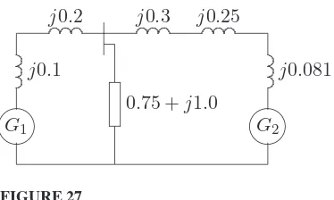
400 = 0.75 +j1.0 pu

The per unit equivalent circuit is shown in Figure 27.

✒✑ ✓✏

G1 j0.1 ... . ... . ... .

✒✑ ✓✏

G2 j0.081 ... . ... . ... . .

. . . ... j0.2

. . ... j0.3

. . ... j0.25

0.75 +j1.0

FIGURE 27

(47)

44 CONTENTS

3.14.The one-line diagram of a power system is shown in Figure 28. The three-phase power and line-line ratings are given below.

G: 80 MVA 22 kV X= 24%

Load: 10 Mvar 4 kV ∆-connected capacitors The three-phase ratings of the three-phase transformer are

Primary: Y-connected 40MVA, 110 kV Secondary: Y-connected 40 MVA, 22 kV Tertiary: ∆-connected 15 MVA, 4 kV

The per phase measured reactances at the terminal of a winding with the second one short-circuited and the third open-circuited are

ZP S = 9.6% 40 MVA, 110 kV / 22 kV ZP T = 7.2% 40 MVA, 110 kV / 4 kV ZST = 12% 40 MVA, 22 kV / 4 kV

Obtain the T-circuit equivalent impedances of the three-winding transformer to the common MVA base. Draw an impedance diagram showing all impedances in per unit on a 100-MVA base. Choose 22 kV as the voltage base for generator.

(48)

is

VB2= 22

µ₂₂₀

22

¶

= 220 kV

This fixes the base on the HV side ofT2atVB3 = 220kV, and on its LV side at

VB4= 220

µ ₂₂

220

¶

= 22 kV

Similarly, the voltage base at buses 5 and 6 are

VB5=VB6 = 22

µ₁₁₀

22

¶

= 110 kV

Voltage base for the tertiary side ofT4is

VBT = 110

µ ₄

110

¶

= 4 kV

The per unit impedances on a 100 MVA base are:

G: X= 0.24

µ₁₀₀

80

¶

= 0.30 pu

T1: X= 0.10

µ₁₀₀

50

¶

= 0.20 pu

T2: X= 0.06

µ₁₀₀

40

¶

= 0.15 pu

T3: X= 0.064

µ₁₀₀

40

¶

= 0.16 pu

The motor reactance is expressed on its nameplate rating of 68.85 MVA, and 20 kV. However, the base voltage at bus 4 for the motor is 22 kV, therefore

M: X= 0.225

µ ₁₀₀

68.85

¶ µ₂₀

22

¶2

= 0.27 pu

Impedance bases for lines 1 and 2 are

ZB2=

(220)2

100 = 484 Ω

ZB5=

(110)2

(49)

46 CONTENTS

. . . . . . . . . . . . . . . . . . . . . . . . . . . .

. ... ... ...

. . . . . . . . . . . . . . . . . . . . . . . . . . . .

. ... ... ... ... .

... .

. ... .

✒✑

✓✏ ...

. ... .

❄Im

✒✑ ✓✏

G M

1 _j₀_.₂₀ _j₀_.₂₅ _j₀_.₁₅ 4

j0.16 j0.35 j0.06 j0.18

j0.3 j0.27

0.12

−j10

Eg Em

✲I

FIGURE 29

Per unit impedance diagram for Problem 3.14.

Line 1 and 2 per unit reactances are Line1: X =

µ₁₂₁

484

¶

= 0.25 pu

Line2: X =

µ

42.35 121

¶

= 0.35 pu The load impedance in ohms is

ZL=

(VL−L)2 S∗

L(3φ)

= (4)

2

j10 =−j1.6 Ω

The base impedance for the load is ZBT =

(4)2

100 = 0.16 Ω

Therefore, the load impedance in per unit is ZL(pu)= −

j1.6

0.16 =−j10 pu

The three-winding impedances on a 100 MVA base are ZP S = 0.096

µ₁₀₀

40

¶

= 0.24 pu

ZP T = 0.072

µ₁₀₀

40

¶

= 0.18 pu

ZST = 0.120

µ₁₀₀

40

¶

(50)

The equivalent T circuit impedances are ZP =

1

2(j0.24 +j0.18−j0.30) =j0.06 pu

ZS =

1

2(j0.24 +j0.30−j0.18) =j0.18 pu

ZT =

1

2(j0.18 +j0.30−j0.24) =j0.12 pu

3.15. The three-phase power and line-line ratings of the electric power system shown in Figure 30 are given below.

. ... .

... .

. . . . . . . . . . . . . . . . . . . . . . . . . . . . . . . . . . . . ... . . . . . . . . . . . . . . . ...

...

... . . . . . . . . . . . . . . . . . . . . . . . . . . . . . . . . . . ... . . . . . . . . . . . ... ✚✙

✛✘

✚✙ ✛✘ G

Vg T1 T2 Vm

M

1 _Line 2

FIGURE 30

G1: 60 MVA 20 kV X = 9%

T1 : 50 MVA 20/200 kV X = 10% T2 : 50 MVA 200/20 kV X = 10% M : 43.2 MVA 18 kV X = 8%

Line: 200 kV Z = 120 +j200 Ω

(a) Draw an impedance diagram showing all impedances in per unit on a 100-MVA base. Choose 20 kV as the voltage base for generator.

(b) The motor is drawing 45 MVA, 0.80 power factor lagging at a line-to-line ter-minal voltage of 18 kV. Determine the terter-minal voltage and the internal emf of the generator in per unit and in kV.

The base voltageV_{B G}1on the LV side ofT1 is 20 kV. Hence the base on its HV side is

VB1= 20

µ₂₀₀

20

¶

= 200 kV

This fixes the base on the HV side ofT2atVB2 = 200kV, and on its LV side at V_{B m}= 200

µ ₂₀

200

¶

(51)

48 CONTENTS

The generator and transformer reactances in per unit on a 100 MVA base, from (3.69)and (3.70) are

G: X= 0.09

µ₁₀₀

60

¶

= 0.15 pu

T1: X= 0.10

µ₁₀₀

50

¶

= 0.20 pu

T2: X= 0.10

µ₁₀₀

50

¶

= 0.20 pu

M: X= 0.08

µ₁₀₀

43.2

¶ µ₁₈

20

¶2

= 0.15 pu

The base impedance for the transmission line is

ZBL=

(200)2

100 = 400 Ω

The per unit line impedance is

Line: Zline= (

120 +j200

400 ) = 0.30 +j0.5 pu

✒✑ ✓✏

Eg

j0.15 Vg

+

−

Vm

+

−

. ... . . . ... . . . ... . .

✒✑ ✓✏

Em

j0.15 ... . ... . ... . .

. ...

j0.2

... 0.3 +j0.5

. . . ... j0.20

FIGURE 31

Per unit impedance diagram for Problem 3.15.

(b) The motor complex power in per unit is

Sm=

456 36.87◦

100 = 0.456 36.87 ◦ _pu

and the motor terminal voltage is

Vm=

186 0◦

(52)

I = 0.456 −36.87◦

0.906 0◦ = 0.56 −36.87◦ pu

Vg = 0.906 0◦+ (0.3 +j0.9)(0.56 −36.87◦ = 1.317956 11.82◦ pu Thus, the generator line-to-line terminal voltage is

Vg = (1.31795)(20) = 26.359 kV

Eg= 0.906 0◦+ (0.3 +j1.05)(0.56 −36.87◦= 1.3756 13.88◦ pu Thus, the generator line-to-line internal emf is

Eg = (1.375)(20) = 27.5 kV

3.16.The one-line diagram of a three-phase power system is as shown in Figure 32. Impedances are marked in per unit on a 100-MVA, 400-kV base. The load at bus2

isS2 = 15.93MW₋j33.4Mvar, and at bus3isS3 = 77MW+j14Mvar. It is required to hold the voltage at bus3at4006 0◦ kV. Working in per unit, determine the voltage at buses2and1.

❄ ❄

V1 V2 V3

S2 S3

j0.5pu j0.4pu

FIGURE 32

S2 = 15.93MW₋j33.4Mvar= 0.1593₋j0.334 pu S3 = 77.00MW+j14.0Mvar= 0.7700 +j0.140 pu V3 =

4006 0◦

400 = 1.06 0 ◦ _pu

I3 = S₃∗ V∗

3

= 0.77−j0.14

1.06 0◦ = 0.77−j0.14 pu

(53)

50 CONTENTS

Therefore, the line-to-line voltage at bus 2 is V2= (400)(1.1) = 440 kV

I2= S∗

2 V₂∗ =

0.1593 +j0.334

1.16 ₋16.26◦ = 0.054 +j0.332 pu

I12= (0.77−j0.14) + (0.054 +j0.332) = 0.824 +j0.192 pu V1= 1.16 16.26◦+ (j0.5)(0.824 +j0.192) = 1.26 36.87◦ pu Therefore, the line-to-line voltage at bus 1 is

V1 = (400)(1.2) = 480 kV

3.17.The one-line diagram of a three-phase power system is as shown in Figure 33. The transformer reactance is20percent on a base of 100-MVA, 23/115-kV and the line impedance isZ =j66.125Ω. The load at bus2isS2 = 184.8MW+j6.6 Mar, and at bus3isS3 = 0MW+j20Mar. It is required to hold the voltage at bus

3at1156 0◦kV. Working in per unit, determine the voltage at buses2and1.

. . ...

❄

V1

V2

V3

S2

S3 j66.125 Ω

FIGURE 33

S2= 184.8MW+j6.6Mvar= 1.848 +j0.066 pu S3= 0MW+j20.0Mvar= 0 +j0.20 pu

V3 =

1156 0◦

115 = 1.06 0 ◦ _pu

I3 = S₃∗ V∗

3

= −j0.2

1.06 0◦ =−j0.2 pu

(54)

Therefore, the line-to-line voltage at bus 2 is

V2= (115)(1.1) = 126.5 kV

I2 = S∗

2 V₂∗ =

1.848₋j0.066

1.16 0◦ = 1.68−j0.06 pu

I12= (1.68−j0.06) + (−j0.2) = 1.68−j0.26 pu V1 = 1.16 0◦+ (j0.2)(1.68−j0.26) = 1.26 16.26◦ pu Therefore, the line-to-line voltage at bus 1 is

(55)

CHAPTER 4 PROBLEMS

4.1.A solid cylindrical aluminum conductor 25 km long has an area of 336,400 circular mils. Obtain the conductor resistance at (a)20◦C and (b)50◦C. The resis-tivity of aluminum at20◦_{C is}₂_.₈_×₁₀−8 _Ω_-m.

(a)

d=√336400 = 580mil= (580)(10−3)(2.54) = 1.4732 cm

A= πd

2

4 = 1.704564 cm

2

R1=ρ ℓ

A = 2.8×10−

8 25×103

1.704564_×10−4 = 4.106 Ω (b)

R2 =R1

µ_{228 + 50}

228 + 20

¶

= 4.106

µ₂₇₈

248

¶

= 4.6 Ω

4.2.A transmission-line cable consists of 12 identical strands of aluminum, each 3 mm in diameter. The resistivity of aluminum strand at20◦C is2.8_×10−8 Ω-m. Find the50◦_{C AC resistance per Km of the cable. Assume a skin-effect correction}

factor of 1.02 at 60 Hz.

(56)

A= 12πd

2

4 = 12

(π)(32₎

4 = 84.823 mm

2

R20=ρ ℓ A =

2.8_×10−8_×₁₀3

84.823_×10−6 = 0.33 Ω

R50=R20

µ_{228 + 50}

228 + 20

¶

= 0.33

µ₂₇₈

248

¶

= 0.37 Ω

RAC= (1.02)(0.37) = 0.3774 Ω

4.3. A three-phase transmission line is designed to deliver 190.5-MVA at 220-kV over a distance of 63 Km. The total transmission line loss is not to exceed

2.5 percent of the rated line MVA. If the resistivity of the conductor material is

2.84_×10−8 _Ω_{-m, determine the required conductor diameter and the conductor} size in circular mils.

The total transmission line loss is

PL=

2.5

100(190.5) = 4.7625 MW

|I_|= √S 3VL

= (190.5)10

3

√

3(220) = 500 A

FromPL= 3R|I|2, the line resistance per phase is

R= 4.7625×10

6

3(500)2 = 6.35 Ω The conductor cross sectional area is

A= (2.84×10−

8₎₍₆₃_×₁₀3₎

6.35 = 2.81764×10 −4 _m2

Therefore

(57)

54 CONTENTS

4.4.A single-phase transmission line 35 Km long consists of two solid round con-ductors, each having a diameter of 0.9 cm. The conductor spacing is 2.5 m. Calcu-late the equivalent diameter of a fictitious hollow, thin-walled conductor having the same equivalent inductance as the original line. What is the value of the inductance per conductor?

4.5.Find the geometric mean radius of a conductor in terms of the radiusrof an individual strand for

(a) Three equal strands as shown in Figure 34(a) (b) Four equal strands as shown in Figure 34(b)

✧✦

Cross section of the stranded conductor for Problem 4.5.

(58)

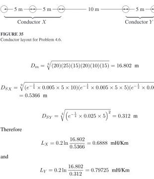
4.6.One circuit of a single-phase transmission line is composed of three solid 0.5-cm radius wires. The return circuit is composed of two solid 2.5-0.5-cm radius wires. The arrangement of conductors is as shown in Figure 35. Applying the concept of theGM D andGM R, find the inductance of the complete line in millihenry per kilometer.

♠ ♠ ♠ ♠ ♠

✛ _{5 m} ✲✛ _{5 m} ✲✛ _{10 m} ✲✛ _{5 m} ✲

| {z }

ConductorX Conductor| {z Y}

FIGURE 35

Conductor layout for Problem 4.6.

Dm = 6

q

(20)(25)(15)(20)(10)(15) = 16.802 m

D_{S X}= 9

q

(e−14 ×0.005×5×10)(e− 1

4 ×0.005×5×5)(e− 1

4 ×0.005×5×10)

= 0.5366 m

DS Y = 4

r ³

e−14 ×0.025×5

´2

= 0.312 m

Therefore

LX = 0.2 ln

16.802

0.5366 = 0.6888 mH/Km

and

LY = 0.2 ln

16.802

0.312 = 0.79725 mH/Km

The loop inductance is

L=LX +LY = 0.6888 + 0.79725 = 1.48605 mH/Km

(59)

56 CONTENTS

♠ ♠ ♠

✛ ✲✛ ✲

✛ ✲

D D

2D

a _b c

FIGURE 36

L= (0.486)10

3

(2π)(60) = 1.2892 mH/Km

Therefore, we have

1.2892 = 0.2 lnGM D

0.02 or GM D= 12.6 m

12.6 = q3 ₍_D₎₍_D₎₍₂_D₎ _or _D_{= 10} _m

4.8.A three-phase transposed line is composed of one ACSR 159,000 cmil, 54/19 Lapwing conductor per phase with flat horizontal spacing of 8 meters as shown in Figure 37. TheGM Rof each conductor is 1.515 cm.

(a) Determine the inductance per phase per kilometer of the line.

(b) This line is to be replaced by a two-conductor bundle with 8-m spacing mea-sured from the center of the bundles as shown in Figure 38. The spacing between the conductors in the bundle is 40 cm. If the line inductance per phase is to be

77 percent of the inductance in part (a), what would be the GM R of each new conductor in the bundle?

♠ ♠ ♠

✛ ✲✛ ✲

✛ ✲

D12= 8m D23= 8m D13= 16m

a b c

FIGURE 37

Conductor layout for Problem 4.8 (a).

(a)

GM D=q3

(8)(8)(16) = 10.0794 m

L= 0.2 10.0794

(60)

❢ ❢ ❢ ❢ ❢ ❢

✛ ✲✛ ✲

✛ ✲

✲ ₄₀ ✛

D12= 8m D23= 8m D13= 16m

a _b c

. . . . . . . . . . . . .

. . . . . . . . . . . . . . . . . . . . . . . . . . . . . . .

. . . . . . . . . . . . . . . . . . . . . . . . . . . . . . . . . . . . . . . . . . . . . . . . . . . . . . . . . . . . .

FIGURE 38

Conductor layout for Problem 4.8 (b).

(b)

L2= (1.3)(0.77) = 1.0 mH/Km

1.0 = 0.2 ln10.0794

Db S

or D_Sb = 0.0679 m

Now

S_Sb =pDSd therefore DS = 1.15cm

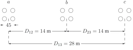
4.9.A three-phase transposed line is composed of one ACSR 1,431,000 cmil, 47/7 Bobolink conductor per phase with flat horizontal spacing of 11 meters as shown in Figure 39. The conductors have a diameter of 3.625 cm and aGM R of 1.439 cm. The line is to be replaced by a three-conductor bundle of ACSR 477,000 cmil, 26/7 Hawk conductors having the same cross-sectional area of aluminum as the single-conductor line. The conductors have a diameter of 2.1793 cm and aGM R of 0.8839 cm. The new line will also have a flat horizontal configuration, but it is to be operated at a higher voltage and therefore the phase spacing is increased to 14 m as measured from the center of the bundles as shown in Figure 40. The spacing between the conductors in the bundle is 45 cm. Determine

(a) The percentage change in the inductance. (b) The percentage change in the capacitance.

♠ ♠ ♠

✛ ✲✛ ✲

✛ ✲

D12= 11m D23= 11m D13= 22m

a b c

FIGURE 39

(61)

58 CONTENTS

❢ ❢❢ ❢ ❢❢ ❢ ❢❢

✛ ✲✛ ✲

✛ ✲

✲ ₄₅ ✛

D12= 14m D23= 14m D13= 28m

a b c

. . . . . . . . . . . . .

. . . . . . . . . . . . . . . . . . . . . . . . . . . . . . .

. . . . . . . . . . . . . . . . . . . . . . . . . . . . . . . . . . . . . . . . . . . . . . . . . . . . . . . . . . . . .

FIGURE 40

Conductor layout for Problem 4.9 (b).

For the one conductor per phase configuration , we have

GM D=q3

(11)(11)(22) = 13.859 m

L= 0.2 13.859

1.439_×10−2 = 1.374 mH/Km

C = 0.0556 ln₁_.₈₁₂₅13.859_×₁₀−2

= 0.008374 µF/Km

For the three-conductor bundle per phase configuration , we have

GM D=q3

(14)(14)(28) = 17.6389 m

GM RL= 3

q

(45)2₍₀_._{8839) = 12}_.₁₄₁₆ _cm

GM RC = 3

q

(45)2₍₂_.₁₇₉₃_/_{2) = 13}_.₀₁₈₇₉ _cm

L= 0.2 17.6389

12.1416_×10−2 = 0.9957 mH/Km

C= 0.0556 ln₁₃_.₀₁₈₇₉17.6389

×10−2

= 0.011326 µF/Km

(a) The percentage reduction in the inductance is

1.374₋0.9957

(62)

(b) The percentage increase in the capacitance is

0.001326₋0.008374

0.008374 (100) = 35.25%

4.10.A single-circuit three-phase transmission transposed line is composed of four ACSR 1,272,000 cmil conductor per phase with horizontal configuration as shown in Figure 41. The bundle spacing is 45 cm. The conductor code name ispheasant.

In MATLAB, use command acsr to find the conductor diameter and its GM R.

Determine the inductance and capacitance per phase per kilometer of the line. Use function[GMD, GMRL, GMRC] =gmd, (4.58) and (4.92) inMATLABto verify your results.

Using the commandacsr, result in

Enter ACSR code name within single quotes -> ’pheasant’ Al Area Strand Diameter GMR Resistance Ohm/Km Ampacity CMILS Al/St cm cm 60Hz,25C 60HZ,50C Ampere 1272000 54/19 3.5103 1.4173 0.04586 0.05290 1200

From (4.79)

GM D=q3 _{(14)(14)(28) = 17}_.₆₃₈₈₉ _m and From (4.53) and (4.90), we have

GM RL= 1.094 and from (4.58) and (4.92), we get

L= 0.2 ln GM D

GM RL = 0.2 ln

17.63889