PRE Book 07 Standard handbook of petroleum and natural gas engineering

(1)

(2)

Petroleum & Natural Gas

Engineering

(3)

(4)

Petroleum & Natural Gas

Engineering

Second Edition

Editors

William C. Lyons, Ph.D., P.E.

Gary J. Plisga, B.S.

AMSTERDAM • BOSTON• HEIDELBERG • LONDON• NEW YORK • OXFORD PARIS • SAN DIEGO • SAN FRANCISCO• SINGAPORE • SYDNEY• TOKYO

(5)

200 Wheeler Road, Burlington, MA 01803, USA Linacre House, Jordan Hill, Oxford OX2 8DP, UK

No part of this publication may be reproduced, stored in a retrieval system, or transmitted in any form or

by any means, electronic, mechanical, photocopying, recording, or otherwise, without the prior written permission of the publisher.

Permissions may be sought directly from Elsevier’s Science & Technology Rights Department in Oxford,

UK: phone: (+44) 1865 843830, fax: (+44) 1865 853333, e-mail: permissions@elsevier.com.uk. You may also complete your request on-line via the Elsevier homepage (http://elsevier.com), by selecting “Customer Support” and then “Obtaining Permissions.”

Recognizing the importance of preserving what has been written, Elsevier prints its books on acid-free paper whenever possible.

Librar y of Congress Cataloging-in-Publication Data

Standard handbook of petroleum & natural gas engineering.—2nd ed./ editors, William C. Lyons, Gary J. Plisga.

p. cm.

Includes bibliographical references and index. ISBN 0-7506-7785-6

1. Petroleum engineering. 2. Natural gas. I. Title: Standard handbook of petroleum and natural gas engineering. II. Lyons, William C. III. Plisga, Gary J.

TN870.S6233 2005 665.5–dc22

2004056285

British Librar y Cataloguing-in-Publication Data

A catalogue record for this book is available from the British Library. ISBN: 0-7506-7785-6

For information on all Gulf Professional Publishing publications visit our Web site at www.gulfpp.com

10 9 8 7 6 5 4 3 2 1

(6)

Contributing Authors vii Preface xi

1 Mathematics 1-1 1.1 General 1-2 1.2 Geometry 1-2 1.3 Algebra 1-6 1.4 Trigonometry 1-8

1.5 Differential and Integral Calculus 1-10 1.6 Analytic Geometry 1-16

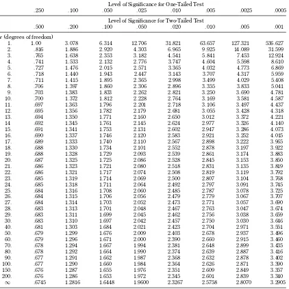
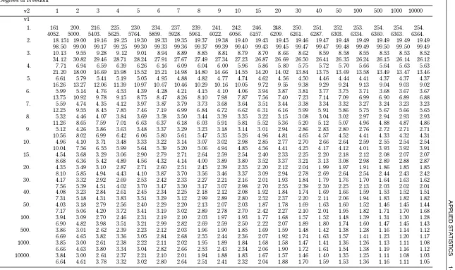
1.7 Numerical Methods 1-20 1.8 Applied Statistics 1-31 1.9 Computer Applications 1-38

2 General Engineering and Science 2-1 2.1 Basic Mechanics (Statics and

Dynamics) 2-2 2.2 Fluid Mechanics 2-19 2.3 Strength of Materials 2-27 2.4 Thermodynamics 2-32 2.5 Geological Engineering 2-69 2.6 Electricity 2-91

2.7 Chemistry 2-100 2.8 Engineering Design 2-129

3 Auxiliar y Equipment 3-1 3.1 Prime Movers 3-2

3.2 Power Transmission 3-17 3.3 Pumps 3-39

3.4 Compressors 3-48

4 Drilling and Well Completions 4-1 4.1 Drilling and Well Servicing Structures 4-2 4.2 Hoisting System 4-9

4.3 Rotary Equipment 4-82 4.4 Mud Pumps 4-95

4.5 Drilling Muds and Completion Fluids 4-103

4.6 Drill String: Composition and Design 4-124 4.7 Bits and Downhole Tools 4-192

4.8 Drilling Mud Hydraulics 4-255 4.9 Underbalanced Drilling and

Completions 4-259 4.10 Downhole Motors 4-276 4.11 MWD and LWD 4-300 4.12 Directional Drilling 4-356

4.13 Selection of Drilling Practices 4-363 4.14 Well Pressure Control 4-371 4.15 Fishing and Abandonment 4-378 4.16 Casing and Casing String Design 4-406 4.17 Well Cementing 4-438

4.18 Tubing and Tubing String Design 4-467 4.19 Corrosion in Drilling and Well

Completions 4-501

4.20 Environmental Considerations for Drilling Operations 4-545

4.21 Offshore Drilling Operations 4-558

5 Reser voir Engineering 5-1

5.1 Basic Principles, Definitions, and Data 5-2 5.2 Formation Evaluation 5-53

5.3 Pressure Transient Testing of Oil and Gas Wells 5-151

5.4 Mechanisms & Recovery of Hydrocarbons by Natural Means 5-158

5.5 Material Balance and Volumetric Analysis 5-161

5.6 Decline Curve Analysis 5-168 5.7 Reserve Estimates 5-172 5.8 Secondary Recovery 5-177 5.9 Fluid Movement in Waterflooded

Reservoirs 5-183

5.10 Estimation of Waterflood Residual Oil Saturation 5-201

5.11 Enhanced Oil Recovery Methods 5-211

6 Production Engineering 6-1 6.1 Properties of Hydrocarbon Mixtures 6-2 6.2 Flow of Fluids 6-40

6.3 Natural Flow Performance 6-89 6.4 Sucker Rod Pumping 6-120

6.5 Stimulation and Remedial Operations 6-218 6.6 Oil and Gas Production Processing

Systems 6-242

6.7 Gas Production Engineering 6-274 6.8 Corrosion in Production Operations 6-371 6.9 Environmental Considerations

in Oil and Gas Operations 6-406 6.10 Offshore Operations 6-424 6.11 Industry Standards for Production

Facilities 6-443

7 Petroleum Economic Evaluation 7-1 7.1 Estimating Producible Volumes and

Future of Production 7-2 7.2 Estimating the Value of Future

Production 7-15

Appendix: Units, Dimensions and Conversion Factors 1

(7)

(8)

Egill Abrahamsen

Weatherford International Limited Houston, Texas

Chip Abrant

Bo Anderson

Robert P. Badrak

Frederick Beck Consultant Denver, Colorado Susan Beck

Joe Berr y Varco Incorporated Houston, Texas Daniel Boone

Consultant in Petroleum Engineering Houston, Texas

Gordon Bopp

Environmental Technology and Educational Services Company

Richland, Washington Ronald Brimhall Consultant

College Station, Texas Ernie Brown Schlumberger Sugarland, Texas Tom Carlson

Halliburton Energy Services Group Houston, Texas

William X. Chavez, Jr.

New Mexico Institute of Mining and Technology Socorro, New Mexico

Francesco Ciulla

Vern Cobb Consultant Robert Colpitts

Consultant in Geology and Geophysics Las Vegas, Nevada

Robert B. Coolidge

Heru Danardatu Schlumberger Balikpapan, Indonesia Tracy Darr van Reet Chevron—retired El Paso, Texas Robert Desbrandes Louisiana State University Baton Rouge, Louisiana Aimee Dobbs Global Santa Fe Houston, Texas Patricia Duettra

Consultant in Applied Mathematics and Computer Analysis

Albuquerque, New Mexico Ernie Dunn

Michael Economides University of Houston Houston, Texas Jason Fasnacht Boart Longyear Salt Lake City, Utah Joel Ferguson

Jerr y W. Fisher

Robert Ford

Smith Bits International Houston, Texas Kazimierz Glowacki

Consultant in Energy and Environmental Engineering Krakow, Poland

Bill Grubb

Mark Heironimus El Paso Production El Paso, Texas Matthew Hill

(9)

Chevron Texaco El Paso, Texas Phillip Johnson University of Alabama Tuscaloosa, Alabama Harald Jordan BP America, Inc. Farmington, New Mexico Mike Juenke

Reza Kashmiri

International Lubrication and Fuel, Incorporated Rio Rancho, New Mexico

William Kersting, MS New Mexico State University Las Cruces, New Mexico Murty Kuntamukkla

Westinghouse Savannah River Company Aiken, South Carolina

Doug LaBombard

Julius Langlinais Louisiana State University Baton Rouge, Louisiana William Lyons

James Martens

F. David Martin Consultant

Albuquerque, New Mexico George McKown Smith Services Houston, Texas David Mildren Dril Tech Mission Fort Worth, Texas Mark Miller Pathfinder Texas

Richard J. Miller

Richard J. Miller and Associates, Incorporated Huntington Beach, California

Stefan Miska University of Tulsa Tulsa, Oklahoma

Global Santa Fe Houston, Texas Abdul Mujeeb

Henkels & McCoy, Incorporated Blue Bell, Pennsylvania Bob Murphy

Tim Parker

Pudji Permadi

Institut Teknologi Bandung Bandung, Indonesia Jim Pipes

Gar y J. Plisga

Consultant in Hydrocarbon Properties Albuquerque, New Mexico

Floyd Preston University of Kansas Lawrence, Kansas Toby Pugh

Carroll Rambin

Bharath N. Rao

President, Bhavya Technologies, Inc. Richard S. Reilly

Cher yl Rofer

Tammoak Enterprises, LLC Los Alamos, New Mexico Chris Russell

Consultant in Environmental Engineering Grand Junction, Colorado

Jorge H.B. Sampaio, Jr.

Eddie Scales National Oil Well Houston, Texas Ron Schmidt

(10)

Richardson, Texas

Paul Singer

New Mexico Institute of Mining and Technology

Socorro, New Mexico

Jack Smith

Mark Trevithick

T&T Engineering Services, Inc. Houston, Texas

Houston, Texas Bill Wamsley Smith Bits International Houston, Texas Sue Weber

Consultant in Computer and Mathematics Jack Wise

(11)

(12)

Several objectives guided the preparation of this second edition of theStandard Handbook of Petroleum and Natu-ral Gas Engineering. As in the first edition, the first objective in this edition was to continue the effort to create for the worldwide petroleum and natural gas exploration and pro-duction industries an engineering handbook written in the spirit of the classic handbooks of the other important engi-neering disciplines. This new edition reflects the importance of these industries to the modern world economies and the importance of the engineers and technicians that serve these industries.

The second objective of this edition was to utilize, nearly exclusively, practicing engineers in industry to carry out the reviews, revisions, and any re-writes of first edition mate-rial for the new second edition. The third objective was, of course, to update the information of the old edition and to make the new edition more SI friendly. The fourth objective was to unite the previous two volumes of the first edition into a single volume that could be available in both book and CD form. The fifth and final objective of the handbook was to maintain and enhance the first edition objective of hav-ing a publication that could be read and understood by any up-to-date engineer or technician, regardless of discipline.

The initial chapters of the handbook set the tone by inform-ing the reader of the common language and notation all engineering disciplines utilize. This common language and notation is used throughout the handbook (in nearly all cases consistent with Society of Petroleum Engineers publi-cation practices). The 75 contributing authors have tried to avoid the jargon that has crept into petroleum engineering literature over the past few decades.

The specific petroleum engineering discipline chapters cover drilling and well completions, reservoir engineering, production engineering, and economics (with valuation and risk analysis). These chapters contain information, data, and example calculations directed toward practical situa-tions that petroleum engineers often encounter. Also, these chapters reflect the growing role of natural gas in the world economies by integrating natural gas topics and related subjects throughout the volume.

The preparation of this new edition has taken approxi-mately two years. Throughout the entire effort the authors have been steadfastly cooperative and supportive of the editors. In the preparation of the handbook the authors

have used published information from both the American Petroleum Institute and the Society of Petroleum Engineers. The authors and editors thank these two institutions for their cooperation. The authors and editors would also like to thank all the petroleum production and service company employees that have assisted in this project. Specifically, edi-tors would like to express their great appreciation to the management and employees of Weatherford International Limited for providing direct support of this revision. The editors would also like to specifically thank management and employees of Burlington Resources Incorporated for their long term support of the students and faculty at the New Mexico Institute of Mining and Technology, and for their assistance in this book. These two companies have exhibited throughout the long preparation period exemplary vision regarding the potential value of this new edition to the industry.

In the detailed preparation of this new edition, the authors and editors would like to specifically thank Raven Gary. She started as an undergraduate student at New Mexico Institute of Mining and Technology in the fall of 2000. She is now a new BS graduate in petroleum engineering and is happily work-ing in the industry. Raven Gary spent her last two years in college reviewing the incoming material from all the authors, checking outline organization, figure and table organization, and references, and communicating with the authors and Elsevier editors. Our deepest thanks go to Raven Gary. The authors and editors would also like to thank Phil Carmical and Andrea Sherman at Elsevier for their very competent preparation of the final manuscript of this new edition. We also thank all those at Elsevier for their support of this project over the past three years.

All the authors and editors know that this work is not per-fect. But we also know that this handbook has to be written. Our greatest hope is that we have given those that will follow us in future editions of this handbook sound basic material to work with.

(13)

(14)

1

Contents

1.1 GENERAL 1-2

1.2 GEOMETRY 1-2

1.3 ALGEBRA 1-6

1.4 TRIGONOMETRY 1-8

1.5 DIFFERENTIAL AND INTEGRAL CALCULUS 1-10

(15)

1.1 GENERAL

See Reference 1 for additional information.

1.1.1 Sets and Functions

Asetis a collection of distinct objects orelements. The inter-section of two sets S and T is the set of elements which belong to Sandwhich also belong to T. Theunion(or inclusive) of S and T is the set of all elements that belong to S or to T (or to both).

Afunctioncan be defined as a set of ordered pairs, denoted as (x, y) such that no two such pairs have the same first element. The element x is referred to as the independent variable, and the element y is referred to as the dependent variable. A function is established when a condition exists that determines y for each x, the condition usually being defined by an equation such as y=f(x) [2].

References

1. Mark’s Standard Handbook for Mechanical Engineers, 8th Edition, Baumeister, T., Avallone, E. A., and Baumeister III, T. (Eds.), McGraw-Hill, New York, 1978.

1.2 GEOMETRY

See References 1 and 2 for additional information.

1.2.1 Angles

Angles can be measured using degrees or with radian mea-sure. Using the degree system of measurement, a circle has 360◦_{, a straight line has 180}◦_{, and a right angle has 90}◦_{. The} radian system of measurement uses the arc length of a unit circle cut off by the angle as the measurement of the angle. In this system, a circle is measured as 2pradians, a straight line ispradians and a right angle isp/2 radians. An angle A is defined asacuteif 0◦ _< _A _< ₉₀◦_,_right_{if A} ₌ ₉₀◦_, andobtuseif 90◦ _< _A_< ₁₈₀◦_{. Two angles are} complemen-taryif their sum is 90◦_{or are}_{supplementary}_{if their sum is} 180◦_{. Angles are}_congruent_{if they have the same} measure-ment in degrees and line segmeasure-ments are congruent if they have the same length. Adihedral angleis formed by two half-planes having the same edge, but not lying in the same plane. Aplane angleis the intersection of a perpendicular plane with a dihedral angle.

1.2.2 Polygons

Apolygonis a closed figure with at least three line segments that lies within a plane. Aregular polygonis a polygon in which all sides and angles are congruent. Two polygons are similarif their corresponding angles are congruent and cor-responding sides are proportional. A segment whose end points are two nonconsecutive vertices of a polygon is a diagonal. Theperimeteris the sum of the lengths of the sides. 1.2.3 Triangles

Atriangleis a three-sided polygon. The sum of the angles of a triangle is equal to 180◦_{. An}_equilateral_{triangle has three} sides that are the same length, anisoscelestriangle has two sides that are the same length, and ascalenetriangle has three sides of different lengths.

Amedianof a triangle is a line segment whose end points are a vertex and the midpoint of the opposite side. Anangle bisectorof a triangle is a median that lies on the ray bisect-ing an angle of the triangle. Thealtitudeof a triangle is a perpendicular segment from a vertex to the opposite side.

Two triangles are congruent if one of the following is given (where S=side length and A=angle measurement): SSS, SAS, AAS, or ASA.

1.2.4 Quadrilaterals

Aquadrilateralis a four-sided polygon.

Atrapezoidhas one pair of opposite parallel sides. A par-allelogramhas both pairs of opposite sides congruent and parallel. The opposite angles are then congruent, and adja-cent angles are supplementary. The diagonals bisect each other and are congruent. A rhombus is a parallelogram whose four sides are congruent and whose diagonals are perpendicular to each other.

Arectangleis a parallelogram having four right angles; therefore, both pairs of opposite sides are congruent. A rectangle whose sides are all congruent is asquare. 1.2.5 Circles and Spheres

If P is a point on a given plane and r is a positive number, thecirclewith center P and radius r is the set of all points of the plane whose distance from P is equal to r. Thesphere with center P and radius r is the set of all points in space whose distance from P is equal to r. Two or more circles (or spheres) with the same P but different values of r are concentric.

Achordof a circle (or sphere) is a line segment whose end points lie on the circle (or sphere). A line which intersects the circle (or sphere) in two points is asecantof the circle (or sphere). Adiameterof a circle (or sphere) is a chord containing the center, and aradiusis a line segment from the center to a point on the circle (or sphere).

The intersection of a sphere with a plane through its center is called agreat circle.

A line that intersects a circle at only one point is atangent to the circle at that point. Every tangent is perpendicular to the radius drawn to the point of intersection. Spheres may have tangent lines or tangent planes.

Pi (p) is the universal ratio of the circumference of any circle to its diameter and is approximately equal to 3.14159. Therefore, the circumference of a circle ispd or 2pr. 1.2.6 Arcs of Circles

Acentral angleof a circle is an angle whose vertex is the center of the circle. If P is the center and A and B are points, not on the same diameter, which lie on C (the circle), the minor arcAB is the union of A, B, and all points on C in the interior of<APB. Themajor arcis the union of A, B, and all points on C on the exterior of<APB. A and B are the end points of the arc and P is the center. If A and B are the end points of a diameter, the arc is a semicircle. Asectorof a circle is a region bounded by two radii and an arc of the circle. 1.2.7 Concurrency

Two or more lines areconcurrentif there is a single point that lies on all of them. The three altitudes of a triangle (if taken as lines, not segments) are always concurrent, and their point of concurrency is called theorthocenter. The angle bisectors of a triangle are concurrent at a point equidistant from their sides, and the medians are concurrent two thirds of the way along each median from the vertex to the opposite side. The point of concurrency of the medians is thecentroid. 1.2.8 Similarity

Two figures with straight sides aresimilarif corresponding angles are congruent and the lengths of corresponding sides are in the same ratio. A line parallel to one side of a triangle divides the other two sides in proportion, producing a second triangle similar to the original one.

1.2.9 Prisms and Pyramids

(16)

any polygon and with triangular sides meeting at a point in a plane parallel to the base.

Prisms and pyramids are described by their bases: a trian-gular prismhas a triangular base, aparallelpipedis a prism whose base is a parallelogram and arectangular parallelpiped is a right rectangular prism. Acubeis a rectangular par-allelpiped all of whose edges are congruent. Atriangular pyramidhas a triangular base, etc. Acircular cylinderis a prism whose base is a circle and acircular coneis a pyramid whose base is a circle.

1.2.10 Coordinate Systems

Each point on a plane may be defined by a pair of numbers. The coordinate system is represented by a line X in the plane (thex-axis) and by a line Y (they-axis) perpendicular to line X in the plane, constructed so that their intersection, theorigin, is denoted by zero. Any point P on the plane can be described by its two coordinates, which form an ordered pair, so that P(x1, y1) is a point whose location corresponds to the real numbers x and y on the x-axis and the y-axis.

If the coordinate system is extended into space, a third axis, thez-axis, perpendicular to the plane of the x1and y1 axes, is needed to represent the third dimension coordinate defining a point P(x1, y1, z1). The z-axis intersects the x and y axes at their origin, zero. More than three dimensions are frequently dealt with mathematically but are difficult to visualize.

Theslopem of a line segment in a plane with end points P1(x1, y1) and P2(x2, y2) is determined by the ratio of the change in the vertical (y) coordinates to the change in the horizontal (x) coordinates or

m=(y2−y1)/(x2−x1)

except that a vertical line segment (the change in x coor-dinates equal to zero) has no slope (i.e., m is undefined). A horizontal segment has a slope of zero. Two lines with the same slope are parallel and two lines whose slopes are negative reciprocals are perpendicular to each other.

Because the distance between two points P1(x1, y1) and P2(x2, y2) is the hypotenuse of a right triangle, the length (L) of the line segment P1P2is equal to

L=(x2−x1)2+(y2−y1)2 1.2.11 Graphs

Agraphis a set of points lying in a coordinate system and a graph of a condition (such as x = y+2) is the set of all points that satisfy the condition. The graph of the slope-intercept equation, y=mx+b, is a straight line which passes through the point (0, b), where b is the y-intercept (x=0) and m is the slope. The graph of the equation

(x−a)2₊₍_y₋_b₎2₌_r2 is a circle with center (a, b) and radius r.

1.2.12 Vectors

Avectoris described on a coordinate plane by adirected seg-mentfrom its initial point to its terminal point. The directed segment represents the fact that every vector determines a magnitude and a direction. A vectorvis not changed when moved around the plane, if its magnitude and angular ori-entation with respect to the x-axis is kept constant. The initial point ofvmay therefore be placed at the origin of the coordinate system andvmay be denoted by

v= a,b

where a is the x-component and b is the y-component of the terminal point. The magnitude may then be determined by

the Pythagorean theorem

v=a2₊_b2

For every pair of vectors (x1, y1) and (x2, y2), thevector sum is given by (x1+x2, y1+y2). Thescalar productof the vector P=(x, y) and a real number (ascalar) r is rP=(rx, ry). Also see the discussion of polar coordinates in the Section “Trigonometry” and Chapter 2, “Basic Mechanics.”

1.2.13 Lengths and Areas of Plane Figures

For definitions of trigonometric functions, see “Trigonome-try.”

● Right triangle(Figure 1.2.1)

c

● _{Any triangle}(Figure 1.2.2)

A

● Rectangle(Figure 1.2.3)

D D

b

a u

area=ab=1/2 • D2_{sin u}

where u=angle between diagonals D, D. ● _{Parallelogram}(Figure 1.2.4)

(17)

● Trapezoid(Figure 1.2.5)

a

u

b h

D₁ D₂

area=1/2 • (a+b)h=1/2 • D1D2sin u where u=angle between diagonals D1and D2 and where bases a and b are parallel. ● Any quadrilateral(Figure 1.2.6)

b

c u

d a

D₁ D2

area=1/2 • D1D2sin u Note:a2₊_b2₊_c2₊_d2₌_D2

1+D22+4 m2

where m=distance between midpoints of D1and D2.

● Circles

area=pr2 ₌ _{1/2 • Cr}₌_{1/4 • Cd}₌_{1/4 •} _p_d2 ₌ 0.785398 d2

where r=radius d=diameter

C=circumference=2pr=pd. ● _Annulus(Figure 1.2.7)

R r

d b

D

area=p(R2₋_r2₎₌_p_(D2₋_d2_)/4₌₂_p_R′_b where R′₌_{mean radius}₌_{1/2 • (R}₊_r) b=R−r

● Sector(Figure 1.2.8) r

A s

area=1/2 • rs=pr2_A/360◦₌_{1/2 • r}2_{rad A} where rad A=radian measure of angle A

s=length of arc=r rad A ● Ellipse(Figure 1.2.9)

x

b

y

y b

a a

area of ellipse=pab

area of shaded segment=xy+ab sin−1_(x/a) length of perimeter of ellipse=p(a+b)K,

where K = (1+1/4 • m2₊_{1/64 • m}4₊_{1/256 •}

m6₊_{. . .}₎

m=(a−b)/(a+b) ● _Hyperbola(Figure 1.2.10)

a

b

A

P

y

a x

For any hyperbola,

shaded area A=ab • ln[(x/a)+(y/b)] For an equilateral hyperbola (a=b), area A=a2_sinh−1_(y/a)₌_a2_cosh−1_(x/a) where x and y are coordinates of point P. ● _Parabola(Figure 1.2.11)

A

h

(18)

shaded area A=2/3 • ch

P

M

T O F

P u

y

In Figure 1.2.12,

length of arc OP=s=1/2 • PT+1/2 • p • ln [cot(1/2 • u) ]

Here c=any chord p=semilatus rectum PT=tangent at P Note:OT=OM=x

1.2.14 Surfaces and Volumes of Solids ● Regular prism(Figure 1.2.13)

h

a

a r

volume=1/2 • nrah=Bh lateral area=nah=Ph where n=number of sides

B=area of base P=perimeter of base ● _{Right circular cylinder}(Figure 1.2.14)

h

r

volume=pr2_h₌_Bh lateral area=2prh=Ph where B=area of base

P=perimeter of base ● Any prism or cylinder(Figure 1.2.15)

h

volume=Bh=Nl lateral area=Ql

where l=length of an element or lateral edge B=area of base

N=area of normal section Q=perimeter of normal section ● Hollow cylinder(right and circular)

volume=ph(R2₋_r2₎₌_p_hb(D₋_b)₌_p_hb(d₊_b)₌

phbD′₌_p_hb(R₊_r) where h=altitude

r, R (d, D)=inner and outer radii (diameters) b=thickness=R−r

D′₌_{mean diam}₌_{1/2 • (d}₊_D)₌_D₋_b₌_d₊_b ● Sphere

volume=V=4/3 • pr3₌_4.188790r3₌_{1/6 •} _p_d3₌ 0.523599d3

area=A=4pr2₌_p_d2 where r=radius

d=2r=diameter=3_6V_/_p₌₁_.₂₄₀₇₀√3 V =3_A_/_p

=0.56419√A ● _{Hollow sphere}, or spherical shell

volume=4/3•p(R3₋_r3₎₌₁_/₆_•_p(_D3₋_d3₎₌₄_p_R2 1t+ 1/3•pt3

where R, r=outer and inner radii D, d=outer and inner diameters

t=thickness=R−r

R1=mean radius=1/2 • (R+r)

● Torus, oranchor ring(Figure 1.2.16)

r

c

volume=2p2_cr2

(19)

References

1. Moise, E. E., and Downs, Jr., F. L.,Geometry, Addison Wesley, Melano Park, 1982.

2. Graening, J.,Geometry, Charles E. Merrill, Columbus, 1980.

1.3 ALGEBRA

See Reference 1.3 for additional information.

1.3.1 Operator Precedence and Notation

Operations in an equation are performed in the following order of precedence:

1. Parenthesis and grouping symbols 2. Exponents

3. Multiplication or division (left to right) 4. Addition or subtraction (left to right) For example:

a+b•c−d3_/_e

will be operated upon (calculated) as if it were written a+(b•c)− [(d3₎_/_e_]

The symbol |a| means “the absolute value of a,” or the numerical value of a regardless of sign, so that

| −2| = |2| =2

The n! means “n factorial” (where n is a whole number) and is the product of the whole numbers 1 to n inclusive, so that and for their product

n

i=1 ai

The notation “x∞y” is read “x varies directly with y” or “x is directly proportional to y,” meaning x=ky where k is some constant. If x∞1/y, then x is inversely proportional to y and x=k/y.

1.3.2 Rules of Addition

a+b=b+a(commutative property) (a+b)+c=a+(b+c)(associative property) a−(−b)=a+b and

a−(x−y+z)=a−x+y−z

(i.e., a minus sign preceding a pair of parentheses operates to reverse the signs of each term within if the parentheses are removed)

1.3.3 Rules of Multiplication and Simple Factoring a•b=b•a (commutative property)

(For higher-order polynomials, see the “Binomial Theo-rem.”) an₊_bn_{is factorable by (a}₊_{b) if n is odd, and}

The numerator and denominator of a fraction may be mul-tiplied or divided by any quantity (other than zero) without altering the value of the fraction, so that, if m=0,

ma+mb+mc

mx+my =

a+b+c x+y

To add fractions, transform each to a common denomina-tor and add the numeradenomina-tors (b, y=0): To multiply fractions (denominators=0):

a

To divide one fraction by another, invert the divisor and multiply:

Except in simple cases (square and cube roots), radical signs are replaced by fractional exponents. If n is odd,

n √

−a= −√n_a

but if n is even, the nth root of−a is imaginary.

1.3.6 Logarithms

The logarithm of a positive number N is the power to which the base must be raised to produce N. So, x=logbN means bx ₌_{N. Logarithms to the base 10, frequently used} in numerical computation, are calledcommonordenary log-arithms, and those to base e, used in theoretical work, are callednatural logarithmsand frequently notated asln. In any case,

(20)

log(an₎

and since 1/M=2.302585, for conversion (ln=loge) ln x=2.3026 log10x

If n is a positive integer, the system is valid without restriction on x and completes with the term nnxn.

Some of the more useful special cases follow [1]:

with corresponding formulas for (1−x)1/2_{, etc., obtained} by reversing the signs of the odd powers of x. Provided |b|<|a|: each term is obtained from the preceding term by adding a constant difference, d. If n is the number of terms, the last term is p=a+(n−1)d, the “average” term is 1/2(a+p) and the sum of the terms is n times the average term or s = n/2(a+p). Thearithmetic meanbetween a and b is (a+b)/2.

In ageometric progression, (a, ar, ar2_{, ar}3_,_{. . .}_{), each term} is obtained from the preceding term by multiplying by a con-stant ratio, r. The nth term is arn−1_{, and the sum of the first} n terms is s=a(rn₋_1)/(r₋₁₎₌_a(1₋_rn_)/(1₋_{r). If r is a} fraction, rn_{will approach zero as n increases and the sum of} n terms will approach a/(1−r) as a limit.

Thegeometric mean, also called the “mean proportional,” between a and b is√ab. Theharmonic meanbetween a and b is 2ab/(a+b).

1.3.9 Sums of the First n Natural Numbers ● To the first power:

1+2+3+. . .+(n−1)+n=n(n+1)/2

● To the second power (squared):

12₊₂2₊_{. . .}₊₍_n₋₁₎2₊_n2₌_n₍_n₊₁₎₍_2n₊₁₎_/₆

● To the third power (cubed): 13

+23

+. . . +(n−1)3+n3

= [n(n+1)/2]2 1.3.10 Solution of Equations in One Unknown

Legitimate operations on equations include addition of any quantity to both sides, multiplication by any quantity of both sides (unless this would result in division by zero), raising both sides to any positive power (if±is used for even roots) and taking the logarithm or the trigonometric functions of both sides.

Anyalgebraic equationmay be written as a polynomial of nth degree in x of the form

a0xn+a1xn−1+a2xn−2+. . .+an−1x+an=0

with, in general, n roots, some of which may be imaginary and some equal. If the polynomial can be factored in the form

(x−p)(x−q)(x−r). . . =0

then p, q, r,. . . are the roots of the equation. If |x| is very large, the terms containing the lower powers of x are least important, while if |x| is very small, the higher-order terms are least significant.

First-degree equations (linear equations) have the form ax+b=c

with the solution x=b−a and the root b−a.

(21)

and the roots

The sum of the roots is−b/a and their product is c/a. Third-degree equations (cubic equations) have the form, after division by the coefficient of the highest-order term,

x3₊_ax2₊_bx₊_c₌₀ Exponential equationsare of the form

ax

=b

with the solution x=(log b)/(log a) and the root (log b)/ (log a). The complete logarithm must be taken, not just the mantissa.

1.3.11 Solution of Systems of Simultaneous Equations A set ofsimultaneous equationsis a system of n equations in n unknowns. The solutions (if any) are the sets of values for the unknowns that satisfy all the equations in the system.

First-degree equations in 2 unknowns are of the form a1x1+b1x2=c1

a2x1+b2x2=c2

The solution is found by multiplication of Equations 1.3.1 and 1.3.2 by some factors that will produce one term in each that will, upon addition of Equations 1.3.1 and 1.3.2, become zero. The resulting equation may then be rearranged to solve for the remaining unknown. For example, by multiply-ing Equation 1.3.1 by a2and Equation 1.3.2 by−a1, adding Equation 1.3.1 and Equation 1.3.2 and rearranging their sum

x2=

a2c1−a1c2 a2b1−a1b2 and by substitution in Equation 1.3.1:

x1=b1c2−b2c1 a2b1−a1b2

A set ofn first-degree equations in n unknownsis solved in a similar fashion by multiplication and addition to eliminate n−1 unknowns and then back substitution.Second-degree equations in 2 unknownsmay be solved in the same way when two of the following are given: the product of the unknowns, their sum or difference, the sum of their squares. For further solutions, see “Numerical Methods.”

1.3.12 Determinants

Determinants of the second order are of the following form and are evaluated as

and of the third order as

and of higher orders, by the general rules as follows. To evaluate a determinant of the nth order, take the elements of the first column with alternate plus and minus signs and

form the sum of the products obtained by multiplying each of these elements by its correspondingminor. The minor corresponding to any element enis the determinant (of the next lowest order) obtained by striking out from the given determinant the row and column containing en.

Some of the general properties of determinants are 1. Columns may be changed to rows and rows to columns. 2. Interchanging two adjacent columns changes the sign of

the result.

3. If two columns are equal or if one is a multiple of the other, the determinant is zero.

4. To multiply a determinant by any number m, multiply all elements of any one column by m.

Systems of simultaneous equations may be solved by the use of determinants using Cramer’s rule. Although the exam-ple is a third-order system, larger systems may be solved by this method. If

1. Benice, D. D., Precalculus Mathematics, 2nd Edition, Prentice Hall, Englewood Cliffs, 1982.

1.4 TRIGONOMETRY

A directed angle may be thought of as an amount of rota-tion rather than a figure. If −→AB is considered the initial position of the ray, which is then rotated about its end point A to form<BAB′_,−→_AB′_{is its terminal position.}

1.4.2 Basic Trigonometric Functions

A trigonometric function can be defined for an angle q between 0◦_{and 90}◦_{by using Figure 1.4.1.}

1.4.3 Trigonometric Properties

sinq=opposite side/hypotenuse=s1/h cosq=adjacent side/hypotenuse=s2/h

(22)

S₂

S₁ h

θ

Figure 1.4.1 Trigonometric functions of angles.

and the reciprocals of the basic functions (where the function =0)

cotangentq=cotq=1/tanq=s2/s1 secantq=secq=1/cosq=h/s2 cosecantq=cscq=1/sinq=h/s1

To reduce an angle to the first quadrant of the unit circle, that is, to a degree measure between 0◦ _{and 90}◦_, see Table 1.4.1. For function values at major angle values, see Tables 1.4.2 and 1.4.3. Relations between functions and the sum or difference of two functions are given in Table 1.4.4. Generally, there will be two angles between 0◦_{and 360}◦_that correspond to the value of a function.

The trigonometric functions sine and cosine can be defined for any real number by using the radian measure of the angle as described in the section on angles. The tan-gent function is defined on every real number except for places where cosine is zero.

1.4.4 Graphs of Trigonometric Functions

Graphs of the sine and cosine functions are identical in shape and periodic with a period of 360◦_{. The sine function graph}

Table 1.4.1 Angle Reduction to First Quadrant If 90◦_<_x_<₁₈₀◦ ₁₈₀◦_<_x_<₂₇₀◦ ₂₇₀◦_<_x_<₃₆₀◦ sin x= +cos(x−90◦₎ ₋_sin(x₋₁₈₀◦₎ ₋_cos(x₋₂₇₀◦₎ cos x= −sin(x−90◦₎ ₋_cos(x₋₁₈₀◦₎ ₊_sin(x₋₂₇₀◦₎ tan x= −cot(x−90◦₎ ₊_tan(x₋₁₈₀◦₎ ₋_cot(x₋₂₇₀◦₎ csc x= +sec(x−90◦₎ ₋_csc(x₋₁₈₀◦₎ ₋_sec(x₋₂₇₀◦₎ sec x= −csc(x−90◦₎ ₋_sec(x₋₁₈₀◦₎ ₊_csc(x₋₂₇₀◦₎ cot x= −tan(x−90◦₎ ₊_cot(x₋₁₈₀◦₎ ₋_tan(x₋₂₇₀◦₎

translated± 90◦_{along the x-axis produces the graph of the} cosine function. The graph of the tangent function is discon-tinuous when the value of tanqis undefined, that is, at odd multiples of 90◦₍_{. . .}_{, 90}◦_{, 270}◦_,_{. . .}_{). For abbreviated graphs} of the sine, cosine, and tangent functions, see Figure 1.4.2.

1.4.5 Inverse Trigonometric Functions

The inverse sine of x (also referred to as the arc sine of x), denoted by sin−1_{x, is the principal angle whose sine is x,} that is,

y=sin−1_{x means sin y}

=x

Inverse functions cos−1_{x and tan}−1_{x also exist for the} cosine of y and the tangent of y. The principal angle for sin−1_{x and tan}−1_{x is an angle a, where}₋₉₀◦ _< _a _< ₉₀◦_, and for cos−1_{x, 0}◦ _<_a_<₁₈₀◦_.

1.4.6 Solution of Plane Triangles

The solution of any part of a plane triangle is determined in general by any other three parts given by one of the following groups, where S is the length of a side and A is the degree measure of an angle:

● AAS ● SAS ● SSS

The fourth group, two sides and the angle opposite one of them, is ambiguous since it may give zero, one, or two solutions. Given an example triangle with sides a, b, and c and angles A, B, and C (A being opposite a, etc., and A+B +C=180◦_{), the fundamental laws relating to the solution} of triangles are

1. Law of sines: a/(sin A)=b/(sin B)=c/(sin C) 2. Law of cosines: c2₌_a2₊_b2₋_{2ab cos C}

1.4.7 Hyperbolic Functions

Thehyperbolic sine, hyperbolic cosine, etc., of any number x are functions related to the exponential function ex_{. Their} def-initions and properties are very similar to the trigonometric functions and are given in Table 1.4.5.

Table 1.4.3 Trigonometric Function Values at Major Angle Values

Values at 30◦ ₄₅◦ ₆₀◦

sin x 1/2 1/2√2 1/2√3

cos x 1/2√3 1/2√2 1/2

tan x 1/3√3 1 √3

csc x 2 √2 2/3√3

sec x 2/3√3 √2 2

cot x √3 1 1/3√3

Table 1.4.2 Trigonometric Function Values by Quadrant

If 0◦_<_x_<₉₀◦ ₉₀◦_<_x_<₁₈₀◦ ₁₈₀◦_<_x_<₂₇₀◦ ₂₇₀◦_<_x_<₃₆₀◦

sin x +0 to+1 +1 to+0 −0 to−1 −1 to−0

cos x +1 to+0 −0 to−1 −1 to−0 +0 to+1

tan x +0 to+∞ −∞to−0 +0 to+∞ −∞to−0

csc x +∞to+1 +1 to+∞ −∞to−1 −1 to−∞

sec x +1 to+∞ −∞to−1 −1 to−∞ +∞to+1

(23)

Table 1.4.4 Relations Between Trigonometric Functions Multiple and Half Angles

tan 2x=(2 tan x)/(1−tan2_x)

(Note: (n)2, . . . are the binomial coefficients) sin(x/2)= ±1/2(1−cos x)

cos(x/2)= ±1/2(1+cos x)

tan(x/2)=(sin x)/(1+cos x)= ±(1−cos x)/(1+cos x)

Three Angles Whose Sum = 180◦

sin A+sin B+sin C=4 cos(A/2) cos(B/2) cos(C/2) cot(A/2)+cot(B/2)+cot(C/2)

=cot(A/2) cot(B/2) cot(C/2)

sin 2A+sin 2B+sin 2C=4 sin A sin B sin C sin 2A+sin 2B−sin 2C=4 cos A cos B sin C

Theinverse hyperbolic functions, sinh−1_{x, etc., are related} to the logarithmic functions and are particularly useful in integral calculus. These relationships may be defined for real numbers x and y as

1.4.8 Polar Coordinate System

Thepolar coordinate systemdescribes the location of a point (denoted as [r,q]) in a plane by specifying a distance r and an angleqfrom the origin of the system. There are several relationships between polar and rectangular coordinates, diagrammed in Figure 1.4.3. From the Pythagorean theorem

r= ±x2₊_y2 Also

sinq=y/r or y=r sinq cosq=x/r or x=r cosq tanq=y/x or q=tan−1₍_y_/_x₎

To convert rectangular coordinates to polar coordinates, given the point (x, y), using the Pythagorean theorem and the preceding equations.

[r,q] =x2₊_y2_,_tan−1₍_y_/_x₎

To convert polar to rectangular coordinates, given the point [r,q]:

(x,y)= [r cosq,r sinq]

For graphic purposes, the polar plane is usually drawn as a series of concentric circles with the center at the origin and radii 1, 2, 3,. . . Rays from the center are drawn at 0◦_{, 15}◦_,

30◦_{, . . . ,}₃₆₀◦_{or 0,}_p_/12,_p_/6,_p_/4_{, . . . ,}₂_p_{radians. The origin}

is called thepole, and points [r,q] are plotted by moving a positive or negative distance r horizontally from the pole, and through an angleqfrom the horizontal. See Figure 1.4.4 withqgiven in radians as used in calculus. Also note that

[r,q] = [−r,q+p]

1.5 DIFFERENTIAL AND INTEGRAL CALCULUS

See References 1–4 for additional information.

1.5.1 Derivatives

Geometrically, the derivative of y=f(x) at any value xn is the slope of a tangent line T intersecting the curve at the point P(x, y). Two conditions applying to differentiation (the process of determining the derivatives of a function) are 1. The primary (necessary and sufficient) condition is that

lim

Dx→0

Dy Dx

exists and is independent of the way in whichDx→0 2. A secondary (necessary, not sufficient) condition is that

lim

Dx→0f(x+Dx)=f(x)

A short table of derivatives will be found in Table 1.5.1.

1.5.2 Higher-Order Derivatives

Thesecond derivativeof a function y=f(x), denoted f′′_(x) or d2_y/dx2_{is the derivative of f}′_{(x) and the}_{third derivative}_, f′′′_{(x) is the derivative of f}′′_{(x). Geometrically, in terms of f(x):} if f′′_(x)_> _{0 then f(x) is concave upwardly, if f}′′_(x)_<_{0 then} f(x) is concave downwardly.

1.5.3 Partial Derivatives

If u=f(x, y,. . .) is a function of two or more variables, thepartial derivativeof u with respect to x, fx(x, y,. . .) or ∂u/∂x, may be formed by assuming x to be the indepen-dent variable and holding (y,. . .) as constants. In a similar manner, fy(x, y,. . .) or∂u/∂y may be formed by holding

(x, . . .) as constants. Second-order partial derivatives of

(24)

sin X 1

0 ₉₀

The sine graph period 360˚

The cosine graph period 360˚

The tangent graph period 360˚

180 270 360

−1

cos X tan X

1 2

0 ₉₀ ₁₈₀ ₂₇₀ ₃₆₀ 0 ₉₀ ₁₈₀ ₂₇₀

−1 −2

−90

Figure 1.4.2 Graphs of the trigonometric functions.

Table 1.4.5 Hyperbolic Functions sinh x=1/2(ex₋_e−x₎

cosh x=1/2(ex₊_e−x₎ tanh x=sinh x/cosh x csch x=1/sinh x sech x=1/cosh x coth x=1/tanh x sinh(−x)= −sinh x cosh(−x)=cosh x tanh(−x)= −tanh x cosh2_x₋_sinh2_x₌₁ 1−tanh2_x₌_sech2_x 1−coth2_x_{= −}_csch2_x

sinh(x±y)=sinh x cosh y±cosh x sinh y cosh(x±y)=cosh x cosh y±sinh x sinh y tanh(x±y)=(tanh x±tanh y)/(1±tanh x tanh y) sinh 2x=2 sinh x cosh x

cosh 2x=cosh2_x₊_sinh2_x tanh 2x=(2 tanh x)/(1+tanh2_x) sinh(x/2)=1/2(cosh x−1) cosh(x/2)=1/2(cosh x+1)

tanh(x/2)=(cosh x−1)/(sinh x)=(sinh x)/(cosh x+1)

fxy(equal to fyx), fyyor as∂2u/∂x2,∂2u/∂x∂y,∂2u/∂y2, and the higher-order partial derivatives are likewise formed.

Implicit functions(i.e., f(x, y)=0) may be solved by the formula

dy dx= −

fx fy at the point in question.

1.5.4 Maxima and Minima

Acritical pointon a curve y=f(x) is a point where y′₌_0, that is, where the tangent to the curve is horizontal. A critical value of x is therefore a value such that f′_(x)₌_{0. All roots of} the equation f′_(x)₌_{0 are critical values of x, and the} corre-sponding values of y are the critical values of the function.

A function f(x) has arelative maximumat x=a if f(x) < f(a) for all values of x (except a) in some open interval containing a and arelative minimumat x=b if f(x)> f(b) for all x (except b) in the interval containing b. At the relative maximum a of f(x), f′_(a)₌_{0, i.e., slope}₌_{0, and f}′′_(a) _<_0, i.e., the curve is downwardly concave at this point, and at the relative minimum b, f′_(b)₌_{0 and f}′′_(b) _> _{0 (upward} concavity). In Figure 1.5.1 A, B, C, and D are critical points and x1, x2, x3, and x4are critical values of x. A and C are maxima, B is a minimum, and D is neither. D, F, G, and H arepoints of inflectionwhere the slope is minimum or maximum. In special cases, such as E, maxima or minima may occur where f′_{(x) is undefined or infinite.}

Y

X

X r

θ

Figure 1.4.3 Polar coordinates.

π

_/

₂

π

_/

₃ π

_/

₄

π

_/

₆

11π

_/

₆

7π

_/

₄ 5π

_/

₃

3π

_/

₂ 4π

_/

₃

5π

_/

₄ 7π

_/

₅ 5π

_/

₆

3π

_/

₄ 2π

_/

₃

π 0

Figure 1.4.4 The polar plane.

(25)

Table 1.5.1 Table of Derivativesa a_{The u and v represent functions of x. All angles are in radians.}

will always have an absolute minimum and an absolute max-imum, and they will be found either at a relative minimum and a relative maximum or at the endpoints of the interval.

1.5.5 Differentials

If y=f(x) andDx andDy are the increments of x and y, respectively, because y+Dy=f(x+Dx), then

Dy=f(x+Dx)−f(x)

AsDx approaches its limit 0 and (since x is the independent variable) dx=Dx

By defining dy and dx separately, it is now possible to write dy

dx =f′(x) as

dy=f′₌₍_x₎_dx

In functions of two or more variables, where f(x, y,. . .)= 0, if dx, dy,. . . are assigned to the independent variables x,

y, . . ., the differential du is given by differentiating term by

term or by taking

du=fx•dx+fy•dy+. . .

expresses the rate of change of u with respect to t, in terms of the separate rates of change of x, y,. . . with respect to t.

Figure 1.5.1 Maxima and minima.

Y

Figure 1.5.2 Radius of curvature in rectangular coordinates.

1.5.6 Radius of Curvature

Theradius of curvatureR of a plane curve at any point P is the distance along the normal (the perpendicular to the tangent to the curve at point P) on the concave side of the curve to thecenter of curvature(Figure 1.5.2). If the equation of the curve is y=f(x)

R=_duds =[1+f′(x)

2_]3/2 f′′(x)

where the rate of change (ds/dx) and the differential of the arc (ds), s being the length of the arc, are defined as

ds

with u being the angle of the tangent at P with respect to the x-axis. (Essentially, ds, dx, and y correspond to the sides of a right triangle.) The curvature K is the rate at which<u is changing with respect to s, and

(26)

θ

Figure 1.5.3 Radius of curvature in polar coordinates.

In polar coordinates (Figure 1.5.3), r=f(q), where r is the radius vector andqis the polar angle, and

ds=dr2₊_r2_d_q2 If the equation of the circle is

R2₌₍_x₋_a)₊₍_y₋_b)2 by differentiation and simplification

a=x−y′[1+(y′)

Theevoluteis the locus of the centers of curvature, with variablesaandb, and the parameter x (y, y′_{, and y}′′ _all being functions of x). If f(x) is the evolute of g(x), g(x) is theinvoluteof f(x).

1.5.7 Indeﬁnite Integrals

Definition:The indefinite integral (antiderivative) may be defined as follows:

f(x)dx=F(x)+C if F(x)=f(x) The constant C is called the constant of integration. Integration by partsmakes use of the differential of a product

where∫v du may be recognizable as a standard form or may be more easily handled than∫u dv.

Integration by transformationmay be useful when, in cer-tain cases, particular transformations of a given integral to one of a recognizable form suggest themselves.

For example, a given integral involving such quantities as

u2₋_a2_, _u2₊_a2_, _or _a2₋_u2

may suggest appropriate trigonometric transformations such as, respectively,

u=a cscq, u=a tanq, or

u=a sinq

Integration by partial fractions is of assistance in the integration of rational fractions. If

ax+b

and A and B are found by use of determinants (see “Alge-bra”), then Integration by tablesis possible if an integral may be put into a form that can be found in a table of integrals, such as the one given in Table 1.5.2. More complete tables may be found in Bois, “Table of Indefinite Integrals,” Dover, and in others.

1.5.8 Deﬁnite Integrals

Thefundamental theorem of calculusstates that if f(x) is the derivative of F(x) and if f(x) is continuous in the interval [a, b], then

b a

f(x)dx=F(b)−F(a)

Geometrically, the integral of f(x)dx over the interval [a, b] is the area bounded by the curve y=f(x) from f(a) to f(b) and the x-axis from x=a to x=b, or the “area under the curve from a to b.”

1.5.9 Properties of Deﬁnite Integrals b of b and its derivative is

f(b)= _dbd b

a f(x)dx To differentiate with respect to a parameter

∂

Some methods of integration of definite integrals are covered in “Numerical Methods.”

1.5.10 Improper Integrals

(27)

Table 1.5.2 Table of Integralsa a_{The u and v represent functions of x.} †_log

It is possible to integrate functions of several variables by using aniterated integral. An iterated integral is solved from the inner integral to the outer, and variables other than the variable of integration are held constant.

f(x,y)dydx= f(x,y)dy

dx

Definite multiple integrals may have variable inner limits of integration with respect to the outer variable of integration:

d c

g(x)

f(x)

F(x,y)dydx

Uses for multiple integrals include finding areas, volumes, and the center of mass.

1.5.12 Differential Equations

Anordinary differential equationcontains a single indepen-dent variable and a single unknown function of that variable, with its derivatives. Apartial differential equationinvolves an unknown function of two or more independent variables, and its partial derivatives. The order of a differential equa-tion is the order of the highest derivative in the equaequa-tion. The general solution of a differential equation of order n is the set of all functions that possess at least n derivatives and satisfy the equation, as well as any auxiliary conditions.

1.5.13 Methods of Solving Ordinary Differential Equations

Forfirst-order equations, if possible, separate the variables, integrate both sides, and add the constant of integration, C. If the equation ishomogeneousin x and y, the value of dy/dx in terms of x and y is of the form dy/dx=f(y/x) and the variables may be separated by introducing new independent variable v=y/x and then

xdv

dx+v=f(v)

The expression f(x, y)dx+F(x, y)dy is anexact differen-tialif Alinear differential equationof the first order such as

dy/dx+f(x)•y=F(x) has the solution

y=e−p _ep_F₍_x₎_dx₊_C _{where P}₌ _f₍_x₎_dx In the class of nonlinear equations known asBernoulli’s equations, where

dy/dx+f(x)•y=F(x)•yn substituting y1−n₌_{v gives}

dv/dx+(1−n)f(x)•v=(1−n)F(x) [n=0 or 1] which is linear in v and x. InClairaut’s equations

y=xp+f(p) where p=dy/dx,

(28)

Some differential equation of thesecond orderand their

where y1is the solution of the previous equation with second term zero.

The preceding two equations are examples of linear dif-ferential equations with constant coefficients and their solu-tions are often found most simply by the use of Laplace transforms [1].

For the linear equation of the nth_order

An(x)dny/dxn+An−1(x)dn−1y/dxn−1+. . .

+A1(x)dy/dx+A0(x)y=E(x) the general solution is

y=u+c1u1+c2u2+. . .+cnun,

where u is any solution of the given equation and u1, u2, . . . ,un form a fundamental system of solutions to the homogeneous equation [E(x)←zero]. A set of functions has linear independence if its Wronskian determinant,

W(x),=0, where functions may be linearly independent when W(x)=0.)

1.5.14 The Laplace Transformation

The Laplace transformationis based on the Laplace inte-gral which transforms a differential equation expressed in terms of time to an equation expressed in terms of a com-plex variables+jw. The new equation may be manipulated algebraically to solve for the desired quantity as an explicit function of the complex variable.

Essentially three reasons exist for the use of the Laplace transformation:

1. The ability to use algebraic manipulation to solve higher-order differential equations

2. Easy handling of boundary conditions

3. The method is suited to the complex-variable theory associated with the Nyquist stability criterion [1]. In Laplace-transformation mathematics, the following symbols and variables are used:

f(t) = a function of time

s = a complex variable of the form (s+jw)

F(s)= the Laplace transform of f, expressed in s, resulting from operating on f(t) with the Laplace integral. L ₌ the Laplace operational symbol, i.e., F(s)=L_[f(t)]. The Laplace integral is defined as

L₌

Table 1.5.3 lists the transforms of some common time-variable expressions.

The transform of a first derivative of f(t) is L

The transform of a second derivative of f(t) is L_[f′′₍_t₎_{] =}_s2_F₍_s₎₋_sf₍₀+₎₋_f′₍₀+₎

Solutions derived by Laplace transformation are in terms of the complex variable s. In some cases, it is necessary to retransform the solution in terms of time, performing an inverse transformation

L−1_F₍_s₎

=f(t)

Just as there is only one direct transform F(s) for any f(t), there is only one inverse transform f(t) for any F(s) and inverse transforms are generally determined through use of tables.

References

(29)

Table 1.5.3 Laplace Transforms

2. Lial, M. L., and Miller, C. D., Essential Calculus with Applications, 2nd Edition, Scott, Foresman and Company, Glenview, 1980.

3. Oakley, C. O.,The Calculus, Barnes and Noble, New York, 1957.

4. Thomas, G. B., and Finney, R. L.,Calculus and Analytic Geometry, 9th Edition, Addison Wesley, Reading, 1995.

1.6 ANALYTIC GEOMETRY

1.6.1 Symmetry

Symmetry exists for the curve of a function about the y-axis if F(x, y)=F(−x, y), about the x-axis if F(x, y)=F(x,−y), about the origin if F(x, y)=F(−x,−y), and about the 45◦ line if F(x, y)=F(y, x).

1.6.2 Intercepts

Intercepts are points where the curve of a function crosses the axes. The x intercepts are found by setting y=0 and the y intercepts by setting x=0.

1.6.3 Asymptotes

As a point P(x, y) on a curve moves away from the region of the origin (Figure 1.6.1a), the distance between P and some fixed line may tend to zero. If so, the line is called an asymptote of the curve. If N(x) and D(x) are polynomials with no common factor, and

y=N(x)/D(x)

where x = c is a root of D(x), then the line x = c is an asymptote of the graph of y.

P′ [c,y]

Figure 1.6.1a Asymptote of a curve.

m

Figure 1.6.1b Slope of a straight line. 1.6.4 Equations of Slope and Straight Lines

1. Equation for slope of line connecting two points (x1, y1) and (x2, y2)

m= y_x2−y1

2−x1 2. Two-point equation (Figure 1.25)

y−y1 x−x1 =

y2−y1 x2−x1 3. Point-slope equation (Figure 1.25)

y−y1=m(x−x1) 4. Slope-intercept equation (Figure 1.6.1b)

y=mx+b

then the equation of the line tangent to the curve at this point is

y−y1=f′(x1)(x−x1)

and the normal to the curve is the line perpendicular to the tangent with slope m2where

m2= −1/m1= −1/f′(x) or

y−y1= −(x−x1)/f′(x1)

1.6.6 Other Forms of the Equation of a Straight Line ● General equation

ax+by+c=0 ● Intercept equation

(30)

m₂= −

m₁=f′_[x]

P₁[x₁, y₁] normal

tangent Y

X 0

y=f [x]

m1₁

Figure 1.6.2 Tangent and normal to a curve.

Y

X [0, b]

θ [a,0]

p

Figure 1.6.3 Equation of a straight line (normal form).

● Normal form (Figure 1.6.3)

x cosq+y sinq−p=0

● Distance d from a straight line (ax+by+c=0) to a point P(x1, y1)

d=ax1+by1+c ±√a2₊_b2

● If u is the angle between ax+by+c=0 and a′x+b′y+ c′₌_{0 then}

cos u= aa′+bb′ ±(a2₊_b2₎₍_a′2₊_b′2₎

1.6.7 Equations of a Circle (Center (h, k)) ● (x−h)2+(y−k)2=r2

● Origin at center

x2₊_y2₌_r2

● General equation

x2₊_y2₊_Dx₊_Ey₊_F₌₀ where center=(−D/2,−E/2)

radius=(D/2)2₊₍_E_/₂₎2₋_F

● Tangent to circle at (x₁, y₁) x1x+y1y+1

2D(x+x1)+ 1

2E(y+y1)+F=0 ● Parametric form, replacing x and y by

x=a cos u and

y=a sin u

Y

X F

P

[h, k]

Figure 1.6.4 Equation of a parabola.

1.6.8 Equations of a Parabola (Figure 1.6.4)

A parabola is the set of points that are equidistant from a given fixed point (the focus) and from a given fixed line (the directrix) in the plane. The key feature of a parabola is that it is second degree in one of its coordinates and first degree in the other.

● (y−k)2=4p(x−h)

● Coordinates of the vertex V(h, k) and of the focus F(h+p, k)

● Origin at vertex

y2₌_4px

● Equation of the directrix x=h−p ● Length of latus rectum

LL′₌_4p ● Polar equation (focus as origin)

r=p/(1−cosq) ● Equation of the tangent to y2=2 px at (x₁, y₁)

y1y=p(x+x1) 1.6.9 Equations of an Ellipse of Eccentricity e

(Figure 1.6.5) ● (x−h)

2 a2 +

(y−k)2

b2 =1

● Coordinates of center C(h, k), of vertices V(h+a, k) and V′_(h₋_{a, k), and of foci F(h}₊_{ae, k) and F}′_(h₋_{ae, k)} ● Center at origin

x2_/_a2₊_y2_/_b2₌₁

● Equation of the directrices x=h±a/e ● Equation of the eccentricity

e= √

a2₋_b2 a <1 ● Length of the latus rectum

LL′₌_2b2_/_a

● Parametric form, replacing x and y by x=a cos u and y=b sin u ● Polar equation (focus as origin)

r=p/(1−e cosq) ● Equation of the tangent at (x₁, y₁)

b2_x

(31)

Y

X

F′ _F

[h, k]

Figure 1.6.5 Ellipse of eccentricity e.

Y

X

Figure 1.6.6 Equation of a hyperbola.

1.6.10 Equations of a Hyperbola (Figure 1.6.6) ● (x−h)

2 a2 −

(y−k)2

b2 =1

● Coordinates of the center C(h, k), of vertices V(h+a, k) and V′_(h₋_{a, k), and of the foci F(h}₊_{ae, k) and F}′_(h₋_ae, k)

● Center at origin

x2_/_a2₋_y2_/_b2₌₁

● Equation of the directrices x=h±a/e ● Equation of the asymptotes

y−k= ±b/a•(x−k) ● Equation of the eccentricity

e= √

a2₊_b2 a >1 ● Length of the latus rectum

LL′₌_2b2_/_a

● Parametric form, replacing x and y

x=a cosh u and y=b sinh u ● Polar equation (focus as origin)

r=p/(1−e cosq) ● Equation of the tangent at (x, y)

b2_x

1x−a2y1y=a2b2

1.6.11 Equations of Three-Dimensional Coordinate Systems (Figure 1.6.7)

● Distance d between two points

d=(x2−x1)2+(y2−y1)2+(z2−z1)2

● Direction cosines of a line

l=cosa, m=cosb, v=cosg

Figure 1.6.7 Three-dimensional coordinate systems.

● Direction numbers, proportional to the direction cosines with k

a=kl, b=km, c=kv 1.6.12 Equations of a Plane

● ax+by+cz+d=0

1.6.13 Equations of a Line ● Intersection of two planes

1.6.14 Equations of Angles

● Between two lines

cosq=l1l2+m1m2+v1v2

and the lines are parallel if cosq=1 or perpendicular if cosq=0

● Between two planes, given by the angle between the normals to the planes.

1.6.15 Equation (Standard Form) of a Sphere (Figure 1.6.8)

(32)

Y

X Z

Figure 1.6.8 Sphere.

Z

Y

X

Figure 1.6.9 Equation of an ellipsoid.

1.6.16 Equation (Standard Form) of an Ellipsoid (Figure 1.6.9)

x2_/_a2₊_y2_/_b2₊_z2_/_c2₌₁

1.6.17 Equations (Standard Form) of Hyperboloids ● Of one sheet (Figure 1.6.10)

x2_/_a2₊_y2_/_b2₋_z2_/_c2₌₁

● Of two sheets (Figure 1.6.11)

x2_/_a2₋_y2_/_b2₋_z2_/_c2₌₁

1.6.18 Equations (Standard Form) of Paraboloids ● Of elliptic paraboloid (Figure 1.6.12)

x2_/_a2₊_y2_/_b2₌_cz

● Of hyperbolic paraboloid (Figure 1.6.13) x2_/_a2₋_y2_/_b2₌_cz

1.6.19 Equation (Standard Form) of an Elliptic Cone (Figure 1.6.14)

x2_/_a2₊_y2_/_b2₋_z2_/_c2₌₀

1.6.20 Equation (Standard Form) of an Elliptic Cylinder (Figure 1.6.15)

x2_/_a2₊_y2_/_b2₌₁

Z

X

Y

Figure 1.6.10 Hyperboloid of one sheet.

Z

Y

Figure 1.6.11 Hyperboloid of two sheets.

Z

Y

X

Figure 1.6.12 Elliptic paraboloid.

Z

X

Y