Economic fluctuations present a recurring problem for economists and policy-makers. This problem is illustrated in Figure 9-1, which shows growth in real GDP for the U.S. economy. As you can see, although the economy experiences long-run growth that averages about 3.5 percent per year, this growth is not at all steady. Recessions—periods of falling incomes and rising unemployment—are frequent. In the recession of 1990, for instance, real GDP fell 2.2 percent from its peak to its trough, and the unemployment rate rose to 7.7 percent. During reces-sions, not only are more people unemployed, but those who are employed have shorter workweeks, as more workers have to accept part-time jobs and fewer workers have the opportunity to work overtime. When recessions end and the economy enters a boom, these effects work in reverse: incomes rise, unemploy-ment falls, and workweeks expand.
Economists call these short-run fluctuations in output and employment the business cycle. Although this term suggests that economic fluctuations are regular and predictable, they are not. Recessions are as irregular as they are common. Sometimes they are close together, such as the recessions of 1980 and 1982. Sometimes they are far apart, such as the recessions of 1982 and 1990.
In Parts II and III of this book, we developed theories to explain how the economy behaves in the long run. Those theories were based on the classical dichotomy—the premise that real variables, such as output and employment, are not affected by what happens to nominal variables, such as the money supply and the price level. Although classical theories are useful for explaining long-run trends, including the economic growth we observe from decade to decade, most economists believe that the classical dichotomy does not hold in the short run and, therefore, that classical theories cannot explain year-to-year fluctuations in output and employment.
Here, in Part IV, we see how economists explain these short-run fluctuations. This chapter begins our analysis by discussing the key differences between the long run and the short run and by introducing the model of aggregate supply
9
Introduction to Economic Fluctuations
C H A P T E RThe modern world regards business cycles much as the ancient Egyptians regarded the overflowing of the Nile.The phenomenon recurs at intervals, it is of great importance to everyone, and natural causes of it are not in sight.
and aggregate demand. With this model we can show how shocks to the econ-omy lead to short-run fluctuations in output and employment.
Just as Egypt now controls the flooding of the Nile Valley with the Aswan Dam, modern society tries to control the business cycle with appropriate eco-nomic policies.The model we develop over the next several chapters shows how monetary and fiscal policies influence the business cycle. We will see that these policies can potentially stabilize the economy or, if poorly conducted, make the problem of economic instability even worse.
9-1
Time Horizons in Macroeconomics
Before we start building a model of short-run economic fluctuations, let’s step back and ask a fundamental question:Why do economists need different models for different time horizons? Why can’t we stop the course here and be content with the classical models developed in Chapters 3 through 8? The answer, as this book has consistently reminded its reader, is that classical macroeconomic theory applies to the long run but not to the short run. But why is this so?
f i g u r e 9 - 1
Percentage change from 4 quarters earlier
10
8
6
4
2
0
⫺2
⫺4
1960 1965
Year
1970 1975 1980 1985 1990 1995 2000
Real GDP growth rate
Average growth rate
Real GDP Growth in the United States Growth in real GDP averages about 3.5 percent per year, as indicated by the orange line, but there are substantial fluctuations around this average. Recessions are periods when the production of goods and services is declining, represented here by negative growth in real GDP.
How the Short Run and Long Run Differ
Most macroeconomists believe that the key difference between the short run and the long run is the behavior of prices.In the long run, prices are flexible and can re-spond to changes in supply or demand. In the short run, many prices are “sticky’’ at some predetermined level. Because prices behave differently in the short run than in the long run, economic policies have different effects over different time horizons.
To see how the short run and the long run differ, consider the effects of a change in monetary policy. Suppose that the Federal Reserve suddenly reduced the money supply by 5 percent. According to the classical model, which almost all economists agree describes the economy in the long run, the money supply affects nominal variables—variables measured in terms of money—but not real variables. In the long run, a 5-percent reduction in the money supply lowers all prices (including nominal wages) by 5 percent whereas all real variables remain the same.Thus, in the long run, changes in the money supply do not cause fluc-tuations in output or employment.
In the short run, however, many prices do not respond to changes in mone-tary policy. A reduction in the money supply does not immediately cause all firms to cut the wages they pay, all stores to change the price tags on their goods, all mail-order firms to issue new catalogs, and all restaurants to print new menus. Instead, there is little immediate change in many prices; that is, many prices are sticky. This short-run price stickiness implies that the short-run impact of a change in the money supply is not the same as the long-run impact.
A model of economic fluctuations must take into account this short-run price stickiness. We will see that the failure of prices to adjust quickly and completely means that, in the short run, output and employment must do some of the adjusting instead. In other words, during the time horizon over which prices are sticky, the classical dichotomy no longer holds: nominal variables can influence real variables, and the economy can deviate from the equilibrium predicted by the classical model.
C A S E S T U D Y
The Puzzle of Sticky Magazine Prices
How sticky are prices? The answer to this question depends on what price we consider. Some commodities, such as wheat, soybeans, and pork bellies, are traded on organized exchanges, and their prices change every minute. No one would call these prices sticky.Yet the prices of most goods and services change much less frequently. One survey found that 39 percent of firms change their prices once a year, and another 10 percent change their prices less than once a year.1
The reasons for price stickiness are not always apparent. Consider, for example, the market for magazines. A study has documented that magazines change their newsstand prices very infrequently. The typical magazine allows inflation to erode
1Alan S. Blinder, “On Sticky Prices: Academic Theories Meet the Real World,’’ in N. G. Mankiw,
The Model of Aggregate Supply
and Aggregate Demand
How does introducing sticky prices change our view of how the economy works? We can answer this question by considering economists’two favorite words— supply and demand.
In classical macroeconomic theory, the amount of output depends on the economy’s ability to supply goods and services, which in turn depends on the supplies of capital and labor and on the available production technology. This is the essence of the basic classical model in Chapter 3, as well as of the Solow growth model in Chapters 7 and 8. Flexible prices are a crucial assumption of classical theory.The theory posits, sometimes implicitly, that prices adjust to en-sure that the quantity of output demanded equals the quantity supplied.
The economy works quite differently when prices are sticky. In this case, as we will see, output also depends on the demandfor goods and services. Demand, in turn, is influenced by monetary policy,fiscal policy, and various other factors. Be-cause monetary and fiscal policy can influence the economy’s output over the time horizon when prices are sticky, price stickiness provides a rationale for why these policies may be useful in stabilizing the economy in the short run.
In the rest of this chapter, we develop a model that makes these ideas more pre-cise.The model of supply and demand, which we used in Chapter 1 to discuss the market for pizza, offers some of the most fundamental insights in economics.This model shows how the supply and demand for any good jointly determine the its real price by about 25 percent before it raises its nominal price.When inflation is 4 percent per year, the typical magazine changes its price about every six years.2
Why do magazines keep their prices the same for so long? Economists do not have a definitive answer.The question is puzzling because it would seem that for magazines, the cost of a price change is small.To change prices, a mail-order firm must issue a new catalog and a restaurant must print a new menu, but a magazine publisher can simply print a new price on the cover of the next issue. Perhaps the cost to the publisher of charging the wrong price is also small. Or maybe cus-tomers would find it inconvenient if the price of their favorite magazine changed every month.
As the magazine example shows, explaining at the microeconomic level why prices are sticky is sometimes hard.The cause of price stickiness is, therefore, an active area of research, which we discuss more fully in Chapter 19. In this chap-ter, however, we simply assume that prices are sticky so we can start developing the link between sticky prices and the business cycle. Although not yet fully ex-plained, short-run price stickiness is widely believed to be crucial for under-standing short-run economic fluctuations.
2Stephen G. Cecchetti,“The Frequency of Price Adjustment: A Study of the Newsstand Prices of
good’s price and the quantity sold, and how shifts in supply and demand affect the price and quantity. In the rest of this chapter, we introduce the “economy-size’’ version of this model—the model of aggregate supply and aggregate demand. This macroeconomic model allows us to study how the aggregate price level and the quantity of aggregate output are determined. It also provides a way to contrast how the economy behaves in the long run and how it behaves in the short run.
Although the model of aggregate supply and aggregate demand resembles the model of supply and demand for a single good, the analogy is not exact. The model of supply and demand for a single good considers only one good within a large economy. By contrast, as we will see in the coming chapters, the model of aggregate supply and aggregate demand is a sophisticated model that incorpo-rates the interactions among many markets.
9-2
Aggregate Demand
Aggregate demand (AD) is the relationship between the quantity of output demanded and the aggregate price level. In other words, the aggregate demand curve tells us the quantity of goods and services people want to buy at any given level of prices.We examine the theory of aggregate demand in detail in Chapters 10 through 12. Here we use the quantity theory of money to provide a simple, although incomplete, derivation of the aggregate demand curve.
The Quantity Equation as Aggregate Demand
Recall from Chapter 4 that the quantity theory says that
MV=PY,
where Mis the money supply,Vis the velocity of money,Pis the price level, and
Y is the amount of output. If the velocity of money is constant, then this equa-tion states that the money supply determines the nominal value of output, which in turn is the product of the price level and the amount of output.
You might recall that the quantity equation can be rewritten in terms of the supply and demand for real money balances:
M/P=(M/P)d=kY,
where k= 1/Vis a parameter determining how much money people want to
hold for every dollar of income. In this form, the quantity equation states that the supply of real money balances M/Pequals the demand (M/P)d and that the de-mand is proportional to output Y. The velocity of money Vis the “flip side”of the money demand parameter k.
For any fixed money supply and velocity, the quantity equation yields a nega-tive relationship between the price level P and output Y. Figure 9-2 graphs the combinations of P and Y that satisfy the quantity equation holding M and V
Why the Aggregate Demand Curve Slopes Downward
As a strictly mathematical matter, the quantity equation explains the downward slope of the aggregate demand curve very simply.The money supply Mand the
velocity of money V determine the nominal value of output PY. Once PY is
fixed, if Pgoes up,Ymust go down.
What is the economics that lies behind this mathematical relationship? For a complete answer, we have to wait for a couple of chapters. For now, however, consider the following logic: Because we have assumed the velocity of money is fixed, the money supply determines the dollar value of all transactions in the economy. (This conclusion should be familiar from Chapter 4.) If the price level rises, each transaction requires more dollars, so the number of transactions and thus the quantity of goods and services purchased must fall.
We can also explain the downward slope of the aggregate demand curve by thinking about the supply and demand for real money balances. If output is higher, people engage in more transactions and need higher real balances M/P.
For a fixed money supply M, higher real balances imply a lower price level.
Con-versely, if the price level is lower, real money balances are higher; the higher level of real balances allows a greater volume of transactions, which means a greater quantity of output is demanded.
Shifts in the Aggregate Demand Curve
The aggregate demand curve is drawn for a fixed value of the money supply. In other words, it tells us the possible combinations of Pand Yfor a given value of M. If the Fed changes the money supply, then the possible combinations of Pand Ychange, which means the aggregate demand curve shifts.
f i g u r e 9 - 2
Price level, P
Income, output, Y Aggregate demand, AD
The Aggregate Demand Curve The aggregate demand curve AD
shows the relationship between the price level Pand the quantity of goods and services demanded
Y. It is drawn for a given value of the money supply M. The aggre-gate demand curve slopes down-ward: the higher the price level P, the lower the level of real balances
For example, consider what happens if the Fed reduces the money supply.The quantity equation,MV = PY, tells us that the reduction in the money supply
leads to a proportionate reduction in the nominal value of output PY. For any given price level, the amount of output is lower, and for any given amount of output, the price level is lower. As in Figure 9-3(a), the aggregate demand curve relating Pand Yshifts inward.
f i g u r e 9 - 3
Price level, P
Income, output, Y (a) Inward Shifts in the Aggregate Demand Curve
AD2 AD1 Reductions in the
money supply shift the aggregate demand curve to the left.
Shifts in the Aggregate Demand Curve Changes in the money supply shift the aggregate mand curve. In panel (a), a de-crease in the money supply M reduces the nominal value of output PY. For any given price level P, output Yis lower. Thus, a decrease in the money supply shifts the aggregate demand curve inward from AD1to AD2. In panel (b), an increase in the money supply Mraises the nomi-nal value of output PY. For any given price level P, output Yis higher. Thus, an increase in the money supply shifts the aggre-gate demand curve outward from AD1to AD2.
Price level, P
Income, output, Y (b) Outward Shifts in the Aggregate Demand Curve
Increases in the money supply shift the aggregate demand curve to the right.
The opposite occurs if the Fed increases the money supply. The quantity equation tells us that an increase in Mleads to an increase in PY. For any given price level, the amount of output is higher, and for any given amount of output, the price level is higher. As shown in Figure 9-3(b), the aggregate demand curve shifts outward.
Fluctuations in the money supply are not the only source of fluctuations in aggregate demand. Even if the money supply is held constant, the aggregate de-mand curve shifts if some event causes a change in the velocity of money. Over the next three chapters, we consider many possible reasons for shifts in the aggre-gate demand curve.
9-3
Aggregate Supply
By itself, the aggregate demand curve does not tell us the price level or the amount of output; it merely gives a relationship between these two variables.To accompany the aggregate demand curve, we need another relationship between P and Y that crosses the aggregate demand curve—an aggregate supply curve. The aggregate demand and aggregate supply curves together pin down the economy’s price level and quantity of output.
Aggregate supply (AS) is the relationship between the quantity of goods and services supplied and the price level. Because the firms that supply goods and services have flexible prices in the long run but sticky prices in the short run, the aggregate supply relationship depends on the time horizon. We need to discuss two different aggregate supply curves: the long-run aggregate supply curve LRASand the short-run aggregate supply curve SRAS.We also need to discuss how the economy makes the transition from the short run to the long run.
The Long Run: The Vertical Aggregate Supply Curve
Because the classical model describes how the economy behaves in the long run, we derive the long-run aggregate supply curve from the classical model. Recall from Chapter 3 that the amount of output produced depends on the fixed amounts of capital and labor and on the available technology. To show this, we write
Y=F(K _
,L _ )
=Y _ .
According to the classical model, output does not depend on the price level.To show that output is the same for all price levels, we draw a vertical aggregate supply curve, as in Figure 9-4.The intersection of the aggregate demand curve with this vertical aggregate supply curve determines the price level.
demand curve shifts downward, as in Figure 9-5.The economy moves from the old intersection of aggregate supply and aggregate demand, point A, to the new intersection, point B.The shift in aggregate demand affects only prices.
The vertical aggregate supply curve satisfies the classical dichotomy, because it implies that the level of output is independent of the money supply. This long-run level of output,Y–, is called the full-employmentor naturallevel of output. It is the level of output at which the economy’s resources are fully employed or, more realistically, at which unemployment is at its natural rate.
f i g u r e 9 - 4
Price level, P
Income, output, Y Long-run aggregate supply, LRAS
Y
The Long-Run Aggregate Supply Curve In the long run, the level of output is determined by the amounts of capital and labor and by the available technology; it does not depend on the price level. The long-run aggregate supply curve, LRAS, is vertical.
f i g u r e 9 - 5
Price level, P
Income, output, Y Y
AD1
AD2 LRAS
A
B
1. A fall in aggregate demand . . .
3. . . . but leaves output the same. 2. . . . lowers
the price level in the long run . . .
Shifts in Aggregate Demand in the Long Run A reduction in the money supply shifts the aggregate demand curve
downward from AD1to AD2.
The Short Run: The Horizontal Aggregate Supply Curve
The classical model and the vertical aggregate supply curve apply only in the long run. In the short run, some prices are sticky and, therefore, do not adjust to changes in demand. Because of this price stickiness, the short-run aggregate sup-ply curve is not vertical.
As an extreme example, suppose that all firms have issued price catalogs and that it is costly for them to issue new ones.Thus, all prices are stuck at predeter-mined levels. At these prices,firms are willing to sell as much as their customers are willing to buy, and they hire just enough labor to produce the amount de-manded. Because the price level is fixed, we represent this situation in Figure 9-6 with a horizontal aggregate supply curve.
f i g u r e 9 - 6
Price level, P
Income, output, Y Short-run aggregate supply, SRAS
The Short-Run Aggregate Supply Curve In this extreme example, all prices are fixed in the short run.
Therefore, the short-run aggregate supply curve, SRAS, is horizontal.
The short-run equilibrium of the economy is the intersection of the aggregate demand curve and this horizontal short-run aggregate supply curve. In this case, changes in aggregate demand do affect the level of output. For example, if the Fed suddenly reduces the money supply, the aggregate demand curve shifts inward, as in Figure 9-7. The economy moves from the old intersection of aggregate de-mand and aggregate supply, point A, to the new intersection, point B.The move-ment from point A to point B represents a decline in output at a fixed price level. Thus, a fall in aggregate demand reduces output in the short run because prices do not adjust instantly.After the sudden fall in aggregate demand,firms are stuck with prices that are too high.With demand low and prices high,firms sell less of their product, so they reduce production and lay off workers. The econ-omy experiences a recession.
From the Short Run to the Long Run
We can summarize our analysis so far as follows:Over long periods of time, prices are
flexible, the aggregate supply curve is vertical, and changes in aggregate demand affect the price level but not output. Over short periods of time, prices are sticky, the aggregate supply curve is
How does the economy make the transition from the short run to the long run? Let’s trace the effects over time of a fall in aggregate demand. Suppose that the economy is initially in long-run equilibrium, as shown in Figure 9-8. In this
figure, there are three curves: the aggregate demand curve, the long-run aggre-gate supply curve, and the short-run aggreaggre-gate supply curve.The long-run equi-librium is the point at which aggregate demand crosses the long-run aggregate supply curve. Prices have adjusted to reach this equilibrium.Therefore, when the
f i g u r e 9 - 7
Price level, P
Income, output, Y
3. . . . lowers the level of output.
2. . . . a fall in aggregate demand . . .
AD1
AD2 SRAS A
B
1. In the short run when prices are sticky. . .
Shifts in Aggregate Demand in the Short Run A reduction in the money supply shifts the
aggregate demand curve downward from AD1to AD2. The equilibrium for the economy moves from point A to point B. Since the aggregate supply curve is horizontal in the short run, the reduction in aggregate demand reduces the level of output.
f i g u r e 9 - 8
Price level, P
Income, output, Y AD
Y
SRAS LRAS
Long-run equilibrium
Long-Run Equilibrium In the long run, the economy finds itself
economy is in its long-run equilibrium, the short-run aggregate supply curve must cross this point as well.
Now suppose that the Fed reduces the money supply and the aggregate de-mand curve shifts downward, as in Figure 9-9. In the short run, prices are sticky, so the economy moves from point A to point B. Output and employment fall below their natural levels, which means the economy is in a recession. Over time, in response to the low demand, wages and prices fall. The gradual reduction in the price level moves the economy downward along the aggregate demand curve to point C, which is the new long-run equilibrium. In the new long-run equilibrium (point C), output and employment are back to their natural levels, but prices are lower than in the old long-run equilibrium (point A).Thus, a shift in aggregate demand affects output in the short run, but this effect dissipates over time as firms adjust their prices.
f i g u r e 9 - 9 Demand The economy begins in long-run equilibrium at point A. A reduction in aggregate mand, perhaps caused by a de-crease in the money supply, moves the economy from point A to point B, where output is below its natural level. As prices fall, the economy gradually re-covers from the recession, mov-ing from point B to point C.
C A S E S T U D Y
Gold, Greenbacks, and the Contraction of the 1870s
The aftermath of the Civil War in the United States provides a vivid example of how contractionary monetary policy affects the economy. Before the war, the United States was on a gold standard. Paper dollars were readily convertible into gold. Under this policy, the quantity of gold determined the money supply and the price level.
9-4
Stabilization Policy
Fluctuations in the economy as a whole come from changes in aggregate sup-ply or aggregate demand. Economists call exogenous changes in these curves shocks to the economy. A shock that shifts the aggregate demand curve is called a demand shock, and a shock that shifts the aggregate supply curve is called a supply shock.These shocks disrupt economic well-being by pushing output and employment away from their natural rates. One goal of the model of aggregate supply and aggregate demand is to show how shocks cause eco-nomic fluctuations.
Another goal of the model is to evaluate how macroeconomic policy can re-spond to these shocks. Economists use the term stabilization policyto refer to policy actions aimed at reducing the severity of short-run economic fl uctua-tions. Because output and employment fluctuate around their long-run natural rates, stabilization policy dampens the business cycle by keeping output and em-ployment as close to their natural rates as possible.
In the coming chapters, we examine in detail how stabilization policy works and what practical problems arise in its use. Here we begin our analysis of stabi-lization policy by examining how monetary policy might respond to shocks. Monetary policy is an important component of stabilization policy because, as we have seen, the money supply has a powerful impact on aggregate demand.
Shocks to Aggregate Demand
Consider an example of a demand shock: the introduction and expanded avail-ability of credit cards. Because credit cards are often a more convenient way to make purchases than using cash, they reduce the quantity of money that people choose to hold.This reduction in money demand is equivalent to an increase in the seigniorage to finance wartime expenditure. Because of this increase in the money supply, the price level approximately doubled during the war.
When the war was over, much political debate centered on the question of whether to return to the gold standard. The Greenback party was formed with the primary goal of maintaining the system of fiat money. Eventually, however, the Greenback party lost the debate. Policymakers decided to retire the green-backs over time in order to reinstate the gold standard at the rate of exchange be-tween dollars and gold that had prevailed before the war.Their goal was to return the value of the dollar to its former level.
the velocity of money.When each person holds less money, the money demand parameter kfalls.This means that each dollar of money moves from hand to hand more quickly, so velocity V(= 1/k) rises.
If the money supply is held constant, the increase in velocity causes nominal spending to rise and the aggregate demand curve to shift outward, as in Figure 9-10. In the short run, the increase in demand raises the output of the economy— it causes an economic boom. At the old prices, firms now sell more output. Therefore, they hire more workers, ask their existing workers to work longer hours, and make greater use of their factories and equipment.
f i g u r e 9 - 1 0 Demand The economy begins in long-run equilibrium at point A. An increase in aggregate de-mand, due to an increase in the velocity of money, moves the economy from point A to point B, where output is above its nat-ural level. As prices rise, output gradually returns to its natural rate, and the economy moves from point B to point C.
Over time, the high level of aggregate demand pulls up wages and prices. As the price level rises, the quantity of output demanded declines, and the economy gradually approaches the natural rate of production. But during the transition to the higher price level, the economy’s output is higher than the natural rate.
What can the Fed do to dampen this boom and keep output closer to the nat-ural rate? The Fed might reduce the money supply to offset the increase in velocity. Offsetting the change in velocity would stabilize aggregate demand.Thus, the Fed can reduce or even eliminate the impact of demand shocks on output and employ-ment if it can skillfully control the money supply.Whether the Fed in fact has the necessary skill is a more difficult question, which we take up in Chapter 14.
Shocks to Aggregate Supply
Because supply shocks have a direct impact on the price level, they are some-times called price shocks. Here are some examples:
➤ A drought that destroys crops.The reduction in food supply pushes up
food prices.
➤ A new environmental protection law that requires firms to reduce their
emissions of pollutants. Firms pass on the added costs to customers in the form of higher prices.
➤ An increase in union aggressiveness.This pushes up wages and the prices
of the goods produced by union workers.
➤ The organization of an international oil cartel. By curtailing competition,
the major oil producers can raise the world price of oil.
All these events are adversesupply shocks, which means they push costs and prices upward. A favorablesupply shock, such as the breakup of an international oil car-tel, reduces costs and prices.
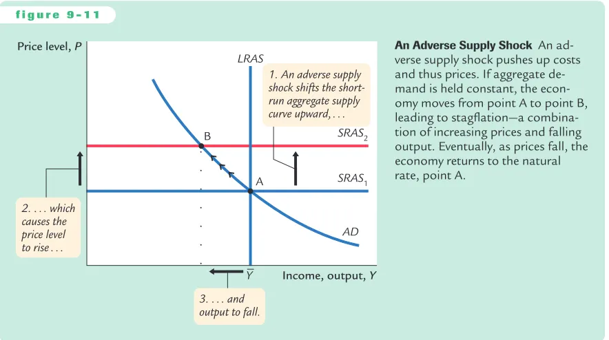
Figure 9-11 shows how an adverse supply shock affects the economy. The short-run aggregate supply curve shifts upward. (The supply shock may also lower the natural level of output and thus shift the long-run aggregate supply curve to the left, but we ignore that effect here.) If aggregate demand is held constant, the economy moves from point A to point B: the price level rises and the amount of output falls below the natural rate. An experience like this is called stagflation, be-cause it combines stagnation (falling output) with inflation (rising prices).
Faced with an adverse supply shock, a policymaker controlling aggregate demand, such as the Fed, has a difficult choice between two options. The first option, implicit in Figure 9-11, is to hold aggregate demand constant. In this case, output and employment are lower than the natural rate. Eventually, prices
f i g u r e 9 - 1 1
An Adverse Supply Shock An ad-verse supply shock pushes up costs and thus prices. If aggregate de-mand is held constant, the econ-omy moves from point A to point B, leading to stagflation—a
will fall to restore full employment at the old price level (point A). But the cost of this adjustment process is a painful recession.
The second option, illustrated in Figure 9-12, is to expand aggregate demand to bring the economy toward the natural rate more quickly. If the increase in ag-gregate demand coincides with the shock to agag-gregate supply, the economy goes immediately from point A to point C. In this case, the Fed is said to accommodate the supply shock.The drawback of this option, of course, is that the price level is permanently higher.There is no way to adjust aggregate demand to maintain full employment and keep the price level stable.
f i g u r e 9 - 1 2 the shock by raising aggregate demand, . . .
Supply Shock In response to
an adverse supply shock, the Fed can increase aggregate de-mand to prevent a reduction in output. The economy moves from point A to point C. The cost of this policy is a perma-nently higher level of prices.
C A S E S T U D Y
How OPEC Helped Cause Stagflation in the 1970s and Euphoria in the 1980s
The most disruptive supply shocks in recent history were caused by OPEC, the Organization of Petroleum Exporting Countries. In the early 1970s, OPEC’s co-ordinated reduction in the supply of oil nearly doubled the world price.This in-crease in oil prices caused stagflation in most industrial countries.These statistics show what happened in the United States:
Change in Inflation Unemployment
Year Oil Prices Rate (CPI) Rate
1973 11.0% 6.2% 4.9%
1974 68.0 11.0 5.6
1975 16.0 9.1 8.5
1976 3.3 5.8 7.7
The 68-percent increase in the price of oil in 1974 was an adverse supply shock of major proportions.As one would have expected, it led to both higher inflation and higher unemployment.
A few years later, when the world economy had nearly recovered from the
first OPEC recession, almost the same thing happened again. OPEC raised oil prices, causing further stagflation. Here are the statistics for the United States:
Change in Inflation Unemployment
Year Oil Prices Rate (CPI) Rate
1978 9.4% 7.7% 6.1%
1979 25.4 11.3 5.8
1980 47.8 13.5 7.0
1981 44.4 10.3 7.5
1982 −8.7 6.1 9.5
The increases in oil prices in 1979, 1980, and 1981 again led to double-digit
in-flation and higher unemployment.
In the mid-1980s, political turmoil among the Arab countries weakened OPEC’s ability to restrain supplies of oil. Oil prices fell, reversing the stagflation of the 1970s and the early 1980s. Here’s what happened:
Change in Inflation Unemployment
Year Oil Prices Rate (CPI) Rate
1983 −7.1% 3.2% 9.5%
1984 −1.7 4.3 7.4
1985 −7.5 3.6 7.1
1986 −44.5 1.9 6.9
1987 l8.3 3.6 6.1
In 1986 oil prices fell by nearly half. This favorable supply shock led to one of the lowest inflation rates experienced in recent U.S. history and to falling un-employment.
More recently, OPEC has not been a major cause of economic fluctuations. This is in part because OPEC has been less successful at raising the price of oil. Although world oil prices have fluctuated, the changes have not been as large as those experienced during the 1970s, and the real price of oil has never returned to the peaks reached in the early 1980s. Moreover, conservation efforts and tech-nological changes have made the economy less susceptible to oil shocks. The amount of oil consumed per unit of real GDP has fallen about 40 percent over the past three decades.
But we should not be too sanguine.The experiences of the 1970s and 1980s could always be repeated. Events in the Middle East are a potential source of shocks to economies around the world.3
3Some economists have suggested that changes in oil prices played a major role in economic fl
9-5
Conclusion
This chapter introduced a framework to study economic fluctuations: the model
of aggregate supply and aggregate demand.The model is built on the assumption
that prices are sticky in the short run and flexible in the long run. It shows how
shocks to the economy cause output to deviate temporarily from the level im-plied by the classical model.
The model also highlights the role of monetary policy. Poor monetary policy can be a source of shocks to the economy. A well-run monetary policy can re-spond to shocks and stabilize the economy.
In the chapters that follow, we refine our understanding of this model and our
analysis of stabilization policy. Chapters 10 through 12 go beyond the quantity
equation to refine our theory of aggregate demand. This refinement shows that
aggregate demand depends on fiscal policy as well as monetary policy. Chapter
13 examines aggregate supply in more detail. Chapter 14 examines the debate over the virtues and limits of stabilization policy.
Summary
1.The crucial difference between the long run and the short run is that prices
are flexible in the long run but sticky in the short run.The model of
aggre-gate supply and aggreaggre-gate demand provides a framework to analyze
eco-nomic fluctuations and see how the impact of policies varies over different
time horizons.
2.The aggregate demand curve slopes downward. It tells us that the lower the
price level, the greater the aggregate quantity of goods and services de-manded.
3.In the long run, the aggregate supply curve is vertical because output is
deter-mined by the amounts of capital and labor and by the available technology, but not by the level of prices.Therefore, shifts in aggregate demand affect the price level but not output or employment.
4.In the short run, the aggregate supply curve is horizontal, because wages and
prices are sticky at predetermined levels. Therefore, shifts in aggregate de-mand affect output and employment.
5.Shocks to aggregate demand and aggregate supply cause economic fl
uctua-tions. Because the Fed can shift the aggregate demand curve, it can attempt to offset these shocks to maintain output and employment at their natural rates.
K E Y C O N C E P T S
Aggregate demand Aggregate supply
Shocks
Demand shocks