STABILITY ANALYSIS OF
NUTRITION-PHYTOPLANKTON-FIRST
SECOND
ZOOPLANKTON-FIRST FISH-SECOND FISH (NPZ
1Z
2F
1F
2)
INTERACTION MODEL
Asrul Sani, Kasliono and Mukhsar
Abstract. The interaction among living organism is commonly found in nature, including in the marine ecosystem, such as the relationship of producers and con-sumers in the form of competition, mutualism and predation. In this study, we develop a mathematical model describing the interactions among species in marine ecosystems, involving five marine species, i.e., phytoplankton, first zooplankton, sec-ond zooplankton, first fish, secsec-ond fish, and the nutritional component. The system has eighteen equilibrium points with fifteen non-negative equilibrium points. The stability criteria for each equilibrium point were derived. Most of the equilibrium points are stable and others are unstable and saddle. Numerical experiments were conducted and they showed the behavior of the system as predicted in the analysis.
1. INTRODUCTION
Not only in terrestrial ecosystems, but also a food chain occurs in marine ecosystems. The food chain shows the feeding relationship among different living things in a particular environment or habitat involving pro-ducers, consumers, and even decomposers [8]. The simplest part of the food
Received 16-12-2016, Accepted 27-12-2016.
2010 Mathematics Subject Classification: 34D20, 34K28
Key words and Phrases: Marine ecosystem, equilibrium point, local stability, numerical experi-ments.
chain is in the form of interaction between preys and predators. The food chain in an ecosystem has served as a natural balance in which a number of species are co-existent in the environment [4].
If a natural unbalance occurs, for instance, the number of predators or the consumer are more than the prey or the producer, it results in a non-equilibrium ecosystem in which the extinction will happen [10, 4]. The interaction among a wide range of species variety in the ocean has been sus-tained for a long time. The interaction itself could have a positive, negative, or no impact among species. The population dynamics of the species due to the interaction is an interesting study.
The marine population dynamics has been extensively studied in many literatures. For example, Stone [14] discussed the interaction of several com-ponents in marine ecosystem, such as bacteria, phytoplankton, zooplankton, protozoa as well as nutrition. Pratikno and Sunarsih [10] studied the in-teraction of three species consisting of prey, first and second predators as a food chain model. In addition, Stone [14] studied three species of the phytoplankton-bacteria-protozoa whereas Edward [3] presented a model of nutrient-phytoplankton-zooplankton. Edward [2] described the relationship between the zooplankton deaths with the dynamics of phytoplankton growth using mathematical modeling approach. It can be seen also in Gross [4] who discussed the role of the food chain as well as Hadley and Forbest [5] viewed the food chain of microorganisms on marine ecosystems through mathemat-ical model. Furthermore, the dynamics of plankton can be found in [11] and that of algae can be seen in [15].
Based on those basic models, Hidayatulloh and Kusumawinahyu [6] introduced a model in a marine ecosystem with five species; nutrients, bac-teria, phytoplankton, zooplankton and protozoa. The discussion of mathe-matical models both in terrestrial and marine ecosystems can be found in [1, 8, 9].
In this study, we developed a mathematical model describing the in-teractions among species in a marine ecosystem which involves six different elements; phytoplankton, first zooplankton, second zooplankton, first fish, second fish and nutrients.
2. MODEL FORMULATION
Suppose P denotes for the population of phytoplankton, Z1 for first
zooplankton,Z2 for second zooplankton,F1 for first fish,F2 for second fish,
model. The dynamics of the food chain in marine ecosystem is far more complex. To simplify the real condition, several following assumptions are introduced.
Assumption
The assumptions relating to the interaction of the six species are as follows.
- Initially, nutrients N are present at the concentrationN0.
- With the presence of nutrition and the absence of predation, Phyto-plankton (P) will grow exponentially with the intrinsic growth rate
r0>0;
dP
dt =r0
N
N0
P.
- The population of phytoplankton will decrease due to predation of zooplankton at rateeaZ1P+ebZ2P and fish at rate egF1P +ekF2P.
The population of first zooplankton decreases due to the predation of second zooplankton at rateecZ2Z1 and fish at rateedF1Z1+eiF2Z1.
Second zooplankton will be consumed by first and second fish at rate
efF1Z2+ejF2Z2 while first fish will be consumed by second fish at
rateehF2F1.
- First and second fish are assumed to die naturally, i.e., at ratedfF1
anddgF2, respectively. In addition, only fish will be assumed to return
as nutrition when they die, i.e., at rate m(dfF1+dgF2).
- The concentration of nutrients will go down as it is consumed by phy-toplankton at ratemr0(N/N0)P.
Schema
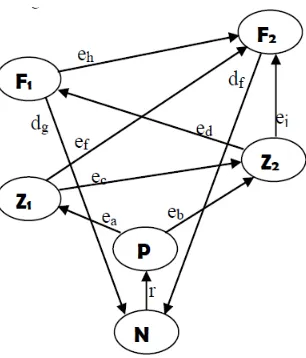
Based on the assumptions, the scheme of the food chain ofN P Z1Z2F1F2 can be described as in Figure 1.
Equation Formulation
Figure 1: The interaction of five species with nutrient in marine ecosystem. The arrow lines show as the predation relationship.
8
where r0 as the growth rate of phytoplankton, ea and eb the grassing
co-efficient of first and second zooplankton on phytoplankton, respectively, ec
for the predation coefficient of second zooplankton on first zooplankton, ed
the predation coefficient of first fish on first zooplankton, ef the predation
coefficient of first fish on second zooplankton, eg the predation coefficient
of first fish on phytoplankton, eh, ei, ej, ek the predation coefficient of
sec-ond fish on first fish, first zooplankton, secsec-ond zooplankton, phytoplankton, respectively; df and dg for the death rate of first concentration of nutrient.
whereα= eb
ea,β=
eg
ea ,γ =
ec
ea ,δ =
ed
ea ,θ=
ef
ea,ε=
df
r0,ω1 =
ek
ea,ω2 =
ei
ea , ω3 = eeja ,ω4 = eeha ,ω5 = drg0 andµ=
m N0
r0
ea.
In the next section, the system of (2) will be analyzed in terms of the stability or the dynamic behaviors of its solution.
3. STABILITY ANALISYS
3.1 Equilibrium Points
The equilibrium pointsE(p, z1, z2, f1, f2, n) of (2) ore obtained by solving:
dp
dτ =
dz1
dτ = (
dz2
dτ =
df1
dτ =
df2
dτ =
dn
dτ = 0, (3)
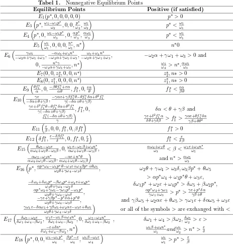
Tabel 1. Nonnegative Equilibrium Points
Equilibrium Points Positive (if satisfied)
E1(p∗,0,0,0,0,0) p∗>0
or all of the symbols> are exchanged with<
E17
J =
a11 a12 a13 a14 a15 a16 a21 a22 a23 a24 a25 a26 a31 a32 a33 a34 a35 a36 a41 a42 a43 a44 a45 a46 a51 a52 a53 a54 a55 a56 a61 a62 a63 a64 a65 a66
(4)
wherea11=n−z1−αz2−βf1−ω1f2,a12=−p,a13=−αp,a14=−βp,a15=
−ω1p,a16=p,a21=z1,a22=p−γz2−δf1−ω2f2,a23=−γz1,a24=−δdz1,
a25 =−ω2z1,a26= 0, a31 =αz2, a32 =γz2, a33=αp+γz1−θf1−ω3f2,
a34 = −θz2, a35 = −ω3z2, a36 = 0, a41 = βf1, a42 = δf1, a43 = θf1,
a44 = βp+ δz1 + θz2 −ω4f2 −ε, a45 = −ω4f1, a46 = 0, a51 = ω1f2,
a52 =ω2f2, a53 =ω3f2,a54 =ω4f2, a55 =ω1p+ω2z1+ω3z2+ω4f1−ω5,
a56= 0,a61=−µn, a62= 0, a63= 0, a64=µε,a65=µω5,a66=−µp.
The stability of nonnegative equilibrium points is obtained by using the linearization approach around those points, i.e., it is a local stability.
• For the equilibrium pointE1. Its Jacobian matrix has the eigenvalues;
λ1=−µp∗,λ2= 0,λ3 =p∗,λ4 =ap∗,λ5 =βp∗−ε,λ6 =−ω5+ω1p∗.
It can be seen that λ4 > 0 for α, p∗ > 0 whereas α5 and α6 can be
negative. Thus, E1 is unstable or saddle.
• All eigenvalues of the Jacobian matrix evaluated inE5 will have
nega-tive real parts if it satisfiesω5 ≤ω2n∗,α5 ≤3 n∗ and β5≤ω4n∗+ǫω1.
Thus, this equilibrium point E5 will be asymptotically local stable if
the above conditions are satisfied.
• The equilibrium pointE7is asymptotically local stable if the following
conditions are satisfied;n∗ ≤α?z∗
2,θz2∗ ≤ǫand ω3z∗2 ≤ω5.
• The equilibrium point E8 has Jacobian matrix with positive real part
of its eigenvalues. Therefore, E8 is asymptotically local unstable.
• The equilibrium point E11 become asymptotically local stable if the
following condition is satisfied;ǫ≤δf∗
1β,αǫ≤θf1∗βandω1ǫ+ω4f1∗β ≤ ω5β.
For the other equilibrium points, i.e.,E3, E4, E6, E9, E10 andE12, their
δω1+ω4
ω2 > β >
ω1ε
ω5 for the nonnegative equilibrium points. Let the values
of the following parameters be fixed; i.e., α = 1, β = 0.5, γ = 1,δ = 0.5,
θ= 2,ε= 4,ω1 = 0.5,ω2 = 0.5,ω3 = 3,ω4= 0.5,ω5 = 6 andµ= 1. Based
on these values, the following equilibrium points are analyzed their stability condition.
• The equilibrium point of E3 should hold p∗ < ωω51 = 12. For the
value p∗ = 4.6, it is obtained that all real parts of its eigenvalues are
positive which means that this equilibrium becomes asymptotically local unstable. As p∗ increases, all real parts of its eigenvalues
be-come negative. Thus, it was concluded that this point E3 becomes
asymptotically local stable if 4.7≤p∗ ≤12.
• The equilibrium point E4 becomes nonnegative if p∗ < ωω51 = 12. For p∗= 0.1, all eigenvalues have negative real part so that the equilibrium
point becomes asymptotically local stable. However, as p∗ = 1.1, it
is obtained that E4 becomes asymptotically local unstable. Thus, the
equilibrium pointE4 is asymptotically local stable when 0≤p∗ ≤1.
• The equilibrium E6 will be nonnegative if 2 = αωω35 < n ∗ < ω5
ω2 = 12. E6 becomes asymptotically local stable for 3≤n∗ <12. For instance,
when n∗ = 2.9 some eigenvalues have positive real parts which means
that E6 is unstable. However, when n∗ = 3 this equilibrium becomes
stable.
• The equilibrium pointE9 means neither first zooplankton nor second
fish are present. This equilibrium will be nonnegative iff∗
1 < εαβθ = 4.
Using the fixed parameters, it is obtained the stability condition 1 < f∗
1 < 4. For instance, when f1∗ = 0.1 some eigenvalues have positive
real parts which means that E9 is unstable. Meanwhile, forf1∗ = 1.1
all eigenvalues have negative real parts, i.e.,E9 is stable.
• The equilibrium point E10 means no second fish exist in the system.
This equilibrium should hold γαε+θf1∗δα
γβθ+θ2 < f1∗ <
γε+δ2
f∗ 1α
δθ+γδβ for
non-negative solution, i.e., 1 < f∗
1 < 4. For f1∗ = 1.1, all real parts of
eigenvalues are negative, which means that E10 is stable whereas for f∗
1 = 3.1 it results in some eigenvalues have positive real parts and
others are negative. This implies that E10 becomes unstable.
• The equilibrium E12 shows that second zooplankton and second fish
value f∗
1, i.e.,f1∗ < δβε = 16. Any values of f1∗ give unstable behavior
around the point E12.
• The equilibriumE17means that the population of second zooplankton
is extinct. The point is nonnegative fore εδ < n∗ < ω5
ω2 or 8< n ∗<12.
For n∗ = 8.1, it results in that all eigenvalues of this equilibrium
point have negative real parts which means that the dynamic behavior around this equilibrium point is stable. It seems that for any n∗ in
8< n∗<12 it will give a stable equilibrium pointE
17.
• The equilibrium pointE18tells that the populations of first and second
zooplankton are extinct and it is nonnegative equilibrium point if the value p∗ belong to where ε
β < p∗ < ω5
ω1 (or 8 < p
∗) . If p∗ = 8.1, it
is found that this equilibrium point is unstable as in the case when
n∗= 11.9. It is concluded that E
18 for anyp∗ belong to 8< p∗.
• The equilibrium point E15 should hold αωω35 < n ∗ < αε
θ for
nonnega-tive solution. It is obtained that the dynamic behavior around this equilibrium point is stable. The equilibrium point E16describes that
all species are present in the system. For nonnegative solution with the fixed parameter values, it holds the condition 1.9≤p∗ ≤2.2. For p∗ = 1.9 and p∗ = 2.1 it is obtained that this equilibrium point is
stable. However, as p∗ = 2.2 it gives an unstable equilibrium Thus,
the stability ofE16 on the interval 1.9≤p∗ ≤2.2 can be both stable
and unstable.
4. NUMERICAL EXPERIMENT
In this study, we perform a numerical simulation for several fixed parameters and allow one or few parameter to vary. Then, we solve nu-merically and compare the results with those in the analysis. The fol-lowing parameters are fixed; namely, α = 1, β = 0.5, γ = 1, δ = 0.5,
θ = 2, ε = 4, ω1 = 0.5, ω2 = 0.5, ω3 = 3, ω4 = 0.5, ω5 = 6 and µ = 1. Using these parameter values with a range of the initial con-centration of nutrition p, it is solved to obtain the nonnegative equilib-rium as follows. For p = 2, we get E1(2,0,0,0,0,0), for p = 4.9, then E3(4.9,7.1,0,0,9.8,12), for p = 1, then E4(1,0,1.833,0,0.333,2), for n =
E8(0,3,0,0,0,4), for f1 = 1, then E9(2,0,1.5,1,0,2), for f1 = 2, then E10(2,2,1,2,0,4) and E12(1,7,0,2,0,8), forf1= 4 then E11(8,0,0,4,0,2),
for n = 9 then E17(2,7,0,3,1,9), for p = 9 then E18(9,0,0,3,1,2).
Fur-thermore, several numerical experiments around the equilibrium points are performed to see the stability behavior of these equilibrium points.
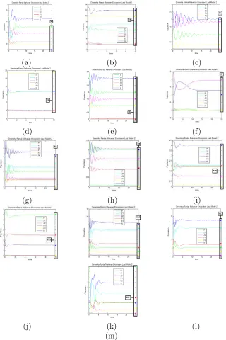
The dynamics of the population around E1 is given in Figure 2(a).
Figure 2(a) shows that the dynamics of the population is away from the equilibrium point E1 which implies that E1 is unstable. The numerical
simulation around the equilibrium point shows that all population does not experience extinction.
The equilibrium point E3 means that the population of second
zoo-plankton and first fish are extinct. The trajectories of the population around
E3 can be seen in Figure 2(b). Figure 2(b) shows that the dynamics of the
population approaches the equilibrium pointE3. Thus, it shows that
equi-librium pointE3 is stable.
The dynamics of the population around the equilibrium point E4 is
given in Figure 2(c). This equilibrium point E4 means that the population
of first zooplankton and first fish are extinct in the long run. The trajectories of the population approach the equilibrium pointE4 which means that it is
stable.
Figure 2(d) shows the behavior of the solution around E5. The
equi-librium point E5 means that the population of first zooplankton, second
zooplankton and first fish are extinct. Numerical simulation around the point E5 shows that the population of first zooplankton, second
zooplank-ton and first fish for the long time will experience extinction, which implies that equilibrium pointE5 is stable.
As shown in Figure 2(e), the equilibrium point E6 is stable. This
equilibrium pointE6 means that the population of first fish is extinct.
Per-turbation aroundE6will initially result in fluctuation all population but all
trajectories return to E6 in the long run. This numerical experiment shows
that equilibrium pointE6 is stable for the determined parameters.
The dynamics of the population around the equilibrium point E7 is
depicted in Figure 2(f). The equilibrium point E7 means that four of the
population is extinct except second zooplankton and nutrition. Numerical solution around the equilibrium point shows that four populations except second zooplankton and nutrition will be extinct for the long time. It shows that equilibrium pointE7 is stable. Figure 2(g) shows the solution behavior
populations except first zooplankton and nutrition are extinct. However, numerical simulation around the equilibrium point shows that all population of do not experience extinction.
The equilibrium pointE9 means that the population of first
zooplank-ton and second fish are extinct. Figure 2(h) shows the dynamics of the population around the equilibrium point E9. numerical simulation of the
system around E9 will for long run return to the equilibrium point. This
indicates that it is stable.
The dynamics of the population around the equilibrium pointE10, as
shown in Figure 2(i), indicates that it is stable. This equilibrium point
E10 means that the population of second fish is extinct. The numerical
experiments around this point show that the trajectories of all population return to the equilibrium point.
As depicted in Figure 2(j) and Figure 2(l), both the equilibrium points
E11 and E17 are stable. The equilibrium point E11 means that the
popula-tion of first and second zooplankton and second fish are extinct, meanwhile, the equilibrium point E17 means that only the population of second
zoo-plankton is extinct. Numerical experiments around these equilibrium points show that all trajectories in both cases return to these equilibrium in the period of 25 unit time.
In the case of E12 and E18, both equilibrium point are unstable as
shown in Figure 2(k) and Figure 2(m). The point E12 means that the
population of second zooplankton and second fish are extinct whereas E18
means that the population of first zooplankton and second zooplankton are extinct. Numerical experiments around these equilibrium points show that all trajectories in both cases are away from these points the period of 25 unit time.
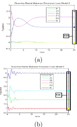
Suppose the parameter values are given as follows; α = 0.5, β = 1,
γ = 1, δ = 0.5,θ= 2, ε= 5, ω1 = 0.5, ω2 = 0.5, ω3 = 2, ω4 = 0.5, ω5 = 5
and µ= 1. These result in the initial population p = 2 and n= 1.25 and give E15(0,0,2.5,0,0,1.25) and E16(2,3,1,1,1,5). The equilibrium point E15 means that the population of first zooplankton is extinct meanwhile
the equilibrium pointE16 means that no populations of species are extinct.
Numerical simulation on equilibrium pointsE15indicates that it is unstable.
Small perturbation around this point causes that the trajectory of second zooplankton is away from its equilibrium. Meanwhile, the small pertur-bation around the equilibrium point E16 shows that the trajectories of all
population are initially oscillate but they go to the equilibrium pointE16in
5. CONCLUSION
In this study we have developed a mathematical model of marine chain food with five marine species; phytoplankton, first zooplankton, second zoo-plankton, first fish, second fish, and the component of nutrition. This system has many equilibrium points and fifteen out of eighteen points are nonneg-ative. The stability of these points is varying in which several equilibrium points have stable behavior whereas others are unstable and saddle. Numer-ical experiments show that the dynamic behaviors around these equilibrium points are in agreement with the analysis. In future, it is interesting to involve more species in the model such that we can get a complete picture describing the rich dynamics of the marine ecosystem as in the real world.
REFERENCES
1. Edelstein-Keshet, L., 1988. Mathematical Models in Biology, Random House, New York, NY, USA,
2. Edwards, A. M., 2001. Adding detritus to a nutrient-phytoplankton-zooplankton model: a dynamical-systems approach, Journal of Plankton Research, 23 (4), 389-413.
3. Edwards, A. M. and Brindley, J., 1999. Zooplankton mortality and the dynamical behaviour of plankton population models, Bulletin of Mathe-matical Biology, 61(2), 303-339.
4. Gross, T., Ebenhoh, W., and Feudel, U., 2004. Enrichment and food-chain stability: the impact of different forms of predator-prey interaction,
Journal of Theoretical Biology, 227(3), 349-358.
5. Hadley, S. and Forbes, L., 2009. Dynamical systems analysis of a two level trophic food web in the Southern Oceans. The ANZIAM Journal, 50, E24-E55.
6. Hidayatulloh, M.R. and Kusumawinahyu, W. M. 2013. Analisis Dinamika Model Rantai Makanan Lima Unsur Ekosistem Laut. Jurusan Matem-atika, FMIPA, Universitas Briwijaya.
7. May, R. M., 2001. Stability and Complexity in Model Ecosystems, Prince-ton University Press, PrincePrince-ton, NJ, USA.
8. Murray, J. D., 1989. Mathematical Biology, vol. 19 of Biomathematics, Springer, New York, NY, USA.
10. Pratikno, W. B. and Sunarsih. 2010. Model Dinamis Rantai Makanan Tiga Spesies. Program Studi Matematika, FMIPA, Universitas Dipone-goro.
11. Ruan, S., 2001. Oscillations in plankton models with nutrient recycling,
Journal of Theoretical Biology, 208(1), 15-26.
12. Seydel, R., 1994. Practical Bifurcation and Stability Analysis: From Equi-librium to Chaos, 2nd edition, Springer, New York, NY, USA.
13. Shertzer, K.W., Ellner, S. P., Fussmann, G. F. and Hairston Jr., N. G., 2002. Predator-prey cycles in an aquatic microcosm: testing hypotheses of mechanism,Journal of Animal Ecology, 71(5), 802-815.
14. Stone, L., 1990. Phytoplankton-bacteria-protozoa-interactions: a quali-tative model portraying indirect effects, Marine Ecology Progress Series, 64, 137-145.
15. Wang, H.L., Feng, J.-F., Shen, F., and Sun, J., 2005. Stability and bifur-cation behaviors analysis in a nonlinear harmful algal dynamical model,
Applied Mathematics and Mechanics, 26(6), 729-734,
Asrul Sani, Kasliono and Mukhsar: Department of Mathematics, FMIPA, Uni-versitas Halu Oleo
(a) (b) (c)
(d) (e) (f)
(g) (h) (i)
(j) (k) (l)
(m)
(a)
(b)