TE
AM
Algorithms and Data
Structures
Julian Bucknall
Tomes of Delphi: algorithms and data structures / by Julian Bucknall. p. cm.
Includes bibliographical references and index. ISBN 1-55622-736-1 (pbk. : alk. paper)
1. Computer software—Development. 2. Delphi (Computer file). 3. Computer algorithms. 4. Data structures (Computer science) I. Title.
QA76.76.D47 .B825 2001 2001033258
005.1--dc21 CIP
© 2001, Wordware Publishing, Inc. Code © 2001, Julian Bucknall
All Rights Reserved
2320 Los Rios Boulevard Plano, Texas 75074
No part of this book may be reproduced in any form or by any means without permission in writing from
Wordware Publishing, Inc.
Printed in the United States of America
ISBN 1-55622-736-1 10 9 8 7 6 5 4 3 2 1 0105
Delphi is a trademark of Inprise Corporation.
Other product names mentioned are used for identification purposes only and may be trademarks of their respective companies.
All inquiries for volume purchases of this book should be addressed to Wordware Publishing, Inc., at the above address. Telephone inquiries may be made by calling:
Introduction . . . x
Chapter 1 What is an Algorithm? . . . 1
What is an Algorithm? . . . 1
Analysis of Algorithms . . . 3
The Big-Oh Notation . . . 6
Best, Average, and Worst Cases . . . 8
Algorithms and the Platform . . . 8
Virtual Memory and Paging . . . 9
Thrashing . . . 10
Locality of Reference . . . 11
The CPU Cache . . . 12
Data Alignment . . . 12
Space Versus Time Tradeoffs . . . 14
Long Strings . . . 16
Use const . . . 17
Be Wary of Automatic Conversions . . . 17
Debugging and Testing . . . 18
Assertions . . . 19
Comments . . . 22
Logging . . . 22
Tracing . . . 22
Coverage Analysis . . . 23
Unit Testing . . . 23
Debugging . . . 25
Summary . . . 26
Chapter 2 Arrays . . . 27
Arrays . . . 27
Array Types in Delphi . . . 28
Standard Arrays . . . 28
Dynamic Arrays . . . 32
New-style Dynamic Arrays . . . 40
TList Class, an Array of Pointers. . . 41
Overview of the TList Class . . . 41
Arrays on Disk . . . 49
Summary . . . 62
Chapter 3 Linked Lists, Stacks, and Queues . . . 63
Singly Linked Lists. . . 63
Linked List Nodes . . . 65
Creating a Singly Linked List . . . 65
Inserting into and Deleting from a Singly Linked List . . . 65
Traversing a Linked List . . . 68
Efficiency Considerations . . . 69
Using a Head Node . . . 69
Using a Node Manager . . . 70
The Singly Linked List Class . . . 76
Doubly Linked Lists . . . 84
Inserting and Deleting from a Doubly Linked List . . . 85
Efficiency Considerations . . . 88
Using Head and Tail Nodes . . . 88
Using a Node Manager . . . 88
The Doubly Linked List Class . . . 88
Benefits and Drawbacks of Linked Lists . . . 96
Stacks . . . 97
Stacks Using Linked Lists . . . 97
Stacks Using Arrays . . . 100
Example of Using a Stack . . . 103
Queues . . . 105
Queues Using Linked Lists . . . 106
Queues Using Arrays . . . 109
Summary . . . 113
Chapter 4 Searching . . . 115
Compare Routines . . . 115
Sequential Search . . . 118
Arrays . . . 118
Linked Lists . . . 122
Binary Search . . . 124
Arrays . . . 124
Linked Lists . . . 126
Inserting into Sorted Containers . . . 129
Summary . . . 131
Chapter 5 Sorting . . . 133
Sorting Algorithms . . . 133
Shuffling a TList . . . 136
Sort Basics . . . 138
Slowest Sorts . . . 138
Bubble Sort. . . 138
Shaker Sort. . . 140
Selection Sort . . . 142
Insertion Sort. . . 144
Fast Sorts . . . 147
Shell Sort. . . 147
Comb Sort . . . 150
Fastest Sorts . . . 152
Merge Sort . . . 152
Quicksort . . . 161
Merge Sort with Linked Lists . . . 176
Summary . . . 181
Chapter 6 Randomized Algorithms . . . 183
Random Number Generation . . . 184
Chi-Squared Tests . . . 185
Middle-Square Method . . . 188
Linear Congruential Method . . . 189
Testing . . . 194
The Uniformity Test . . . 195
The Gap Test . . . 195
The Poker Test . . . 197
The Coupon Collector’s Test . . . 198
Results of Applying Tests . . . 200
Combining Generators . . . 201
Additive Generators . . . 203
Shuffling Generators . . . 205
Summary of Generator Algorithms . . . 207
Other Random Number Distributions . . . 208
Skip Lists . . . 210
Searching through a Skip List . . . 211
Insertion into a Skip List . . . 215
Deletion from a Skip List . . . 218
Full Skip List Class Implementation. . . 219
Summary . . . 225
Chapter 7 Hashing and Hash Tables . . . 227
Hash Functions . . . 228
Simple Hash Function for Strings . . . 230
The PJW Hash Functions . . . 230
Collision Resolution with Linear Probing . . . 232
Advantages and Disadvantages of Linear Probing . . . 233
Deleting Items from a Linear Probe Hash Table . . . 235
The Linear Probe Hash Table Class . . . 237
Other Open-Addressing Schemes . . . 245
Pseudorandom Probing . . . 246
Double Hashing . . . 247
Collision Resolution through Chaining . . . 247
Advantages and Disadvantages of Chaining . . . 248
The Chained Hash Table Class . . . 249
Collision Resolution through Bucketing . . . 259
Hash Tables on Disk . . . 260
Extendible Hashing . . . 261
Summary . . . 276
Chapter 8 Binary Trees . . . 277
Creating a Binary Tree . . . 279
Insertion and Deletion with a Binary Tree . . . 279
Navigating through a Binary Tree . . . 281
Pre-order, In-order, and Post-order Traversals . . . 282
Level-order Traversals . . . 288
Class Implementation of a Binary Tree . . . 289
Binary Search Trees . . . 295
Insertion with a Binary Search Tree. . . 298
Deletion from a Binary Search Tree . . . 300
Class Implementation of a Binary Search Tree . . . 303
Binary Search Tree Rearrangements . . . 304
Splay Trees . . . 308
Class Implementation of a Splay Tree. . . 309
Red-Black Trees . . . 312
Insertion into a Red-Black Tree . . . 314
Deletion from a Red-Black Tree . . . 319
Summary . . . 329
Chapter 9 Priority Queues and Heapsort . . . 331
The Priority Queue . . . 331
First Simple Implementation . . . 332
Second Simple Implementation . . . 335
The Heap . . . 337
Insertion into a Heap . . . 338
Deletion from a Heap . . . 338
Implementation of a Priority Queue with a Heap. . . 340
Heapsort . . . 345
Floyd’s Algorithm . . . 345
Completing Heapsort . . . 346
Extending the Priority Queue . . . 348
Re-establishing the Heap Property . . . 349
Finding an Arbitrary Item in the Heap . . . 350
Implementation of the Extended Priority Queue . . . 350
Summary . . . 356
Chapter 10 State Machines and Regular Expressions . . . 357
State Machines . . . 357
Using State Machines: Parsing . . . 357
Parsing Comma-Delimited Files . . . 363
Deterministic and Non-deterministic State Machines. . . 366
Regular Expressions . . . 378
Using Regular Expressions . . . 380
Parsing Regular Expressions . . . 380
Compiling Regular Expressions . . . 387
Matching Strings to Regular Expressions. . . 399
Summary . . . 407
Chapter 11 Data Compression . . . 409
Representations of Data . . . 409
Data Compression . . . 410
Types of Compression . . . 410
Bit Streams . . . 411
Minimum Redundancy Compression. . . 415
Shannon-Fano Encoding . . . 416
Huffman Encoding . . . 421
Splay Tree Encoding. . . 435
Dictionary Compression . . . 445
LZ77 Compression Description . . . 445
Encoding Literals Versus Distance/Length Pairs . . . 448
LZ77 Decompression . . . 449
LZ77 Compression . . . 456
Summary . . . 467
Chapter 12 Advanced Topics. . . 469
Readers-Writers Algorithm . . . 469
Producers-Consumers Algorithm. . . 478
Single Producer, Single Consumer Model . . . 478
Single Producer, Multiple Consumer Model. . . 486
Finding Differences between Two Files . . . 496
Calculating the LCS of Two Strings . . . 497
Calculating the LCS of Two Text Files. . . 511
Summary . . . 514
Epilogue . . . 515
References . . . 516
You’ve just picked this book up in the bookshop, or you’ve bought it, taken it home and opened it, and now you’re wondering…
Why a Book on Delphi Algorithms?
Although there are numerous books on algorithms in the bookstores, few of them go beyond the standard Computer Science 101 course to approach algo-rithms from a practical perspective. The code that is shown in the book is to illustrate the algorithm in question, and generally no consideration is given to real-life, drop-in-and-use application of the technique being discussed. Even worse, from the viewpoint of the commercial programmer, many are text-books to be used in a college or university course and hence some of the more interesting topics are left as exercises for the reader, with little or no answers.
Of course, the vast majority of them don’t use Delphi, Kylix, or Pascal. Some use pseudocode, some C, some C++, some the languagedu jour; and the most celebrated and referenced algorithms book uses an assembly language that doesn’t even exist (the MIX assembly language inThe Art of Computer Programming[11,12,13]—see the references section). Indeed, those books that do have the word “practical” in their titles are for C, C++, or Java. Is that such a problem? After all, an algorithm is an algorithm is an algorithm; surely, it doesn’t matter how it’s demonstrated, right? Why bother buying and reading one based on Delphi?
Delphi is, I contend, unique amongst the languages and environments used in application development today. Firstly, like Visual Basic, Delphi is an environ-ment for developing applications rapidly, for either 16-bit or 32-bit Windows, or, using Kylix, for Linux. With dexterous use of the mouse, components rain on forms like rice at a wedding. Many double-clicks later, together with a lit-tle typing of code, the components are wedded together, intricately and intimately, with event handlers, hopefully producing a halfway decent-looking application.
Secondly, like C++, Delphi can get close to the metal, easily accessing the various operating system APIs. Sometimes, Borland produces units to access APIs and sells them with Delphi itself; sometimes, programmers have to pore
x
TE
AM
FL
Y
over C header files in an effort to translate them into Delphi (witness the Jedi project at http://www.delphi-jedi.org). In either case, Delphi can do the job and manipulate the OS subsystems to its own advantage.
Delphi programmers do tend to split themselves into two camps: applications programmers and systems programmers. Sometimes you’ll find programmers who can do both jobs. The link between the two camps that both sets of pro-grammers must come into contact with and be aware of is the world of algorithms. If you program for any length of time, you’ll come to the point where you absolutely need to code a binary search. Of course, before you reach that point, you’ll need a sort routine to get the data in some kind of order for the binary search to work properly. Eventually, you might start using a profiler, identify a problem bottleneck in TStringList, and wonder what other data structure could do the job more efficiently.
Algorithms are the lifeblood of the work we do as programmers. Beginner programmers are often afraid of formal algorithms; I mean, until you are used to it, even the word itself can seem hard to spell! But consider this: a program can be defined as an algorithm for getting information out of the user and producing some kind of output for her.
The standard algorithms have been developed and refined by computer scien-tists for use in the programming trenches by the likes of you and me.
Mastering the basic algorithms gives you a handle on your craftandon the language you use. For example, if you know about hash tables, their strengths and weaknesses, what they are used for and why, and have an implementa-tion you could use at a moment’s notice, then you will look at the design of the subsystem or application you’re currently working on in a new light, and identify places where you could profitably use one. If sorts hold no terrors for you, you understand how they work, and you know when to use a selection sort versus a quicksort, then you’ll be more likely to code one in your applica-tion, rather than try and twist a standard Delphi component to your needs (for example, a modern horror story: I remember hearing about someone who used a hidden TListBox component, adding a bunch of strings, and then setting the Sorted property to true to get them in order).
“OK,” I hear you say, “writing about algorithms is fine, but why bother with Delphi or Kylix?”
So, why Delphi? Well, two reasons: the Object Pascal language and the oper-ating system. Delphi’s language has several constructs that are not available in other languages, constructs that make encapsulating efficient algorithms and data structures easier and more natural. Things like properties, for exam-ple. Exceptions for when unforeseen errors occur. Although it is perfectly possible to code standard algorithms in Delphiwithoutusing these Delphi-specific language constructs, it is my contention that we miss out on the beauty and efficiency of the language if we do. We miss out on the ability to learn about the ins and outs of the language. In this book, we shall deliber-ately be using the breadth of the Object Pascal language in Delphi—I’m not concerned that Java programmers who pick up this book may have difficulty translating the code. The cover says Delphi, and Delphi it will be.
And the next thing to consider is that algorithms, as traditionally taught, are generic, at least as far as CPUs and operating systems are concerned. They can certainly be optimized for the Windows environment, or souped up for Linux. They can be made more efficient for the various varieties of Pentium processor we use, with the different types of memory caches we have, with the virtual memory subsystem in the OS, and so on. This book pays particular attention to these efficiency gains. We won’t, however, go as far as coding everything in Assembly language, optimized for the pipelined architecture of modern processors—I have to draw the line somewhere!
So, all in all, the Delphi community does have need for an algorithms book, and one geared for their particular language, operating system, and proces-sor. This is such a book. It was not translated from another book for another language; it was written from scratch by an author who works with Delphi every day of his life, someone who writes library software for a living and knows about the intricacies of developing commercial ready-to-run routines, classes, and tools.
What Should I Know?
This book does not attempt to teach you Delphi programming. You will need to know the basics of programming in Delphi: creating new projects, how to write code, compiling, debugging, and so on. I warn you now: there are no components in this book. You must be familiar with classes, procedure and method references, untyped pointers, the ubiquitous TList, and streams as encapsulated by Delphi’s TStream family. You must have some understanding of object-oriented concepts such as encapsulation, inheritance, polymor-phism, and delegation. The object model in Delphi shouldn’t scare you!
Having said that, a lot of the concepts described in this book are simple in the extreme. A beginner programmer should find much in the book to teach him
or her the basics of standard algorithms and data structures. Indeed, looking at the code should teach such a programmer many tips and tricks of the advanced programmer. The more advanced structures can be left for a rainy day, or when you think you might need them.
So, essentially, you need to have been programming in Delphi for a while. Every now and then you need some kind of data structure beyond what TList and its family can give you, but you’re not sure what’s available, or even how to use it if you found one. Or, you want a simple sort routine, but the only reference book you can find has code written in C++, and to be honest you’d rather watch paint dry than translate it. Or, you want to read an algorithms book where performance and efficiency are just as prominent as the descrip-tion of the algorithm. This book is for you.
Which Delphi Do I Need?
Are you ready for this? Any version. With the exception of the section discuss-ing dynamic arrays usdiscuss-ing Delphi 4 or above and Kylix in Chapter 2, and parts of Chapter 12, and little pieces here and there, the code will compile and run with any version of Delphi. Apart from the small amount of the version-specific code I have just mentioned, I have tested all code in this book with all versions of Delphi and with Kylix.
You can therefore assume that all code printed in this book will work with every version of Delphi. Some code listings are version-specific though, and have been so noted.
What Will I Find, and Where?
This book is divided into 12 chapters and a reference section.
Chapter 1 lays out some ground rules. It starts off by discussing performance. We’ll look at measurement of the efficiency of algorithms, starting out with the big-Oh notation, continuing with timing of the actual run time of algo-rithms, and finishing with the use of profilers. We shall discuss data
representation efficiency in regard to modern processors and operating sys-tems, especially memory caches, paging, and virtual memory. After that, the chapter will talk about testing and debugging, topics that tend to be glossed over in many books, but that are, in fact, essential to all programmers.
Chapter 3 introduces linked lists, both the singly and doubly linked varieties. We’ll see how to create stacks and queues by implementing them with both singly linked lists and arrays.
Chapter 4 talks about searching algorithms, especially the sequential and the binary search algorithms. We’ll see how binary search helps us to insert items into a sorted array or linked list.
Chapter 5 covers sorting algorithms. We will look at various types of sorting methods: bubble, shaker, selection, insertion, Shell sort, quicksort, and merge sort. We’ll also sort arrays and linked lists.
Chapter 6 discusses algorithms that create or require random numbers. We’ll see pseudorandom number generators (PRNGs) and show a remarkable sorted data structure called a skip list, which uses a PRNG in order to help balance the structure.
Chapter 7 considers hashing and hash tables, why they’re used, and what benefits and drawbacks they have. Several standard hashing algorithms are introduced. One problem that occurs with hash tables is collisions; we shall see how to resolve this by using a couple of types of probing and also by chaining.
Chapter 8 presents binary trees, a very important data structure in wide gen-eral use. We’ll look at how to build and maintain a binary tree and how to traverse the nodes in the tree. We’ll also address its unbalanced trees created by inserting data in sorted order. A couple of balancing algorithms will be shown: splay trees and red-black trees.
Chapter 9 deals with priority queues and, in doing so, shows us the heap structure. We’ll consider the important heap operations, bubble up and trickle down, and look at how the heap structure gives us a sort algorithm for free: the heapsort.
Chapter 10 provides information about state machines and how they can be used to solve a certain class of problems. After some introductory examples with finite deterministic state machines, the chapter considers regular expres-sions, how to parse them and compile them to a finite non-deterministic state machine, and then apply the state machine to accept or reject strings.
Chapter 11 squeezes in some data compression techniques. Algorithms such as Shannon-Fano, Huffman, Splay, and LZ77 will be shown.
Chapter 12 includes a variety of advanced topics that may whet your appetite for researching algorithms and structures. Of course, they still will be useful to your programming requirements.
Finally, there is a reference section listing references to help you find out more about the algorithms described in this book; these references not only include other algorithms books but also academic papers and articles.
What Are the Typographical Conventions?
Normal text is written in this font, at this size. Normal text is used for discus-sions, descriptions, and diversions.
Code listings are written in this font, at this size.
Emphasized words or phrases, new words about to be defined, and variables will appear initalic.
Dotted throughout the text are World Wide Web URLs and e-mail addresses which are italicized and underlined, like this:http://www.boyet.com/dads.
Every now and then there will be a note like this. It’s designed to bring out some important point in the narrative, a warning, or a caution.
What Are These Bizarre $IFDEFs in the Code?
The code for this book has been written, with certain noted exceptions, to compile with Delphi 1, 2, 3, 4, 5, and 6, as well as with Kylix 1. (Later com-pilers will be supported as and when they come out; please see
http://www.boyet.com/dadsfor the latest information.) Even with my best efforts, there are sometimes going to be differences in my code between the different versions of Delphi and Kylix.
The answer is, of course, to $IFDEF the code, to have certain blocks compile with certain compilers but not others. Borland supplied us with the official WINDOWS, WIN32, and LINUX compiler defines for the platform, and the VERnnn compiler defined for the compiler version.
To solve this problem, every source file for this book has an include at the top:
{$I TDDefine.inc}
This include file defines human-legible compiler defines for the various com-pilers. Here’s the list:
DelphiN define for a particular Delphi version, N = 1,2,3,4,5,6 DelphiNPlus define for a particular Delphi version or later, N = 1,2,3,4,5,6 KylixN define for a particular Kylix version, N = 1
I also make the assumption that every compiler except Delphi 1 has support for long strings.
What about Bugs?
This book is a book of human endeavor, written, checked, and edited by human beings. To quote Alexander Pope inAn Essay on Criticism, “To err is human, to forgive, divine.” This book will contain misstatements of facts, grammatical errors, spelling mistakes, bugs, whatever, no matter how hard I try going over it withFowler’s Modern English Usage, a magnifying glass, and a fine-toothed comb. For a technical book like this, which presents hard facts permanently printed on paper, this could be unforgivable.
Hence, I shall be maintaining an errata list on my Web site, together with any bug fixes to the code. Also on the site you’ll find other articles that go into greater depth on certain topics than this book. You can always find the latest errata and fixes at http://www.boyet.com/dads. If you do find an error, I would be grateful if you would send me the details by e-mail to
[email protected]. I can then fix it and update the Web site.
There are several people without whom this book would never have been completed. I’d like to present them in what might be termed historical order, the order of their influence on me.
The first two are a couple of gentlemen I’ve never met or spoken to, and yet who managed to open my eyes to and kindle my enthusiasm for the world of algorithms. If they hadn’t, who knows where I might be now and what I might be doing. I’m speaking of Donald Knuth (http://www-cs-staff.stanford. edu/~knuth/) and Robert Sedgewick (http://www.cs.princeton.edu/~rs/). In fact, it was the latter’sAlgorithms[20] that started me off, it being the first algorithms book I ever bought, back when I was just getting into Turbo
Pascal. Donald Knuth needs no real introduction. His masterlyThe Art of Com-puter Programming[11,12,13] remains at the top of the algorithms tree; I first used it at Kings College, University of London while working toward my B.Sc. Mathematics degree.
Fast forwarding a few years, Kim Kokkonen is the next person I would like to thank. He gave me my job at TurboPower Software ( http://www.turbo-power.com) and gave me the opportunity to learn more computer science than I’d ever dreamt of before. A big thank you, of course, to all TurboPower’s employees and those TurboPower customers I’ve gotten to know over the years. I’d also like to thank Robert DelRossi, our president, for encouraging me in this endeavor.
Next is a small company, now defunct, called Natural Systems. In 1993, they produced a product called Data Structures for Turbo Pascal. I bought it, and, in my opinion, it wasn’t very good. Oh, it worked fine, but I just didn’t agree with its design or implementation and it just wasn’t fast enough. It drove me to write my freeware EZSTRUCS library for Borland Pascal 7, from which I derived EZDSL, my well-known freeware data structures library for Delphi. This effort was the first time I’d really gotten tounderstanddata structures, since sometimes it is only through doing that you get to learn.
Thanks also to Chris Frizelle, the editor and owner ofThe Delphi Magazine
succumbing to giving me my own monthly column:Algorithms Alfresco. With-out him and his support, this bookmight have been written, but it certainly wouldn’t have been as good. I certainly recommend a subscription toThe Delphi Magazine, as it remains, in my view, the most in-depth, intelligent ref-erence for Delphi programmers. Thanks to all my readers, as well, for their suggestions and comments on the column.
Next to last, thanks to all the people at Wordware ( http://www.word-ware.com), including my editors, publisher Jim Hill, and developmental edi-tor Wes Beckwith. Jim was a bit dubious at first when I proposed publishing a book on algorithms, but he soon came round to my way of thinking and has been very supportive during its gestation. I’d also like to give my warmest thanks to my tech editors: Steve Teixeira, the co-author of the tome on how to get the best out of Delphi,Delphi n Developer’s Guide(where, at the time of writing, n = 5), and my friend Anton Parris.
Finally, my thanks and my love go to my wife, Donna (she chivvied me to write this book in the first place). Without her love, enthusiasm, and encour-agement, I’d have given up ages ago. Thank you, sweetheart. Here’s to the next one!
Julian M. Bucknall
Colorado Springs, April 1999 to February 2001
What is an Algorithm?
What is an Algorithm?
For a book on algorithms, we have to make sure that we know what we are going to be discussing. As we’ll see, one of the main reasons for understand-ing and researchunderstand-ing algorithms is to make our applications faster. Oh, I’ll agree that sometimes we need algorithms that are more space efficient rather than speed efficient, but in general, it’s performance we crave.
Although this book is about algorithms and data structures and how to imple-ment them in code, we should also discuss some of the procedural algorithms as well: how to write our code to help us debug it when it goes wrong, how to test our code, and how to make sure that changes in one place don’t break something elsewhere.
What is an Algorithm?
What is an Algorithm?
As it happens, we use algorithms all the time in our programming careers, but we just don’t tend to think of them as algorithms: “They’re not algorithms, it’s just the way things are done.”
Analgorithmis a step-by-step recipe for performing some calculation or pro-cess. This is a pretty loose definition, but once you understand that
algorithms are nothing to be afraid of per se, you’ll recognize and use them without further thought.
Go back to your elementary school days, when you were learning addition. The teacher would write on the board a sum like this:
and then ask you to add them up. You had been taught how to do this: start with the units column and add the 5 and the 7 to make 12, put the 2 under the units column, and then carry 1 above the 4.
1
45 17 +
2
You’d then add the carried 1, the 4 and the other 1 to make 6, which you’d then write underneath the tens column. And, you’d have arrived at the con-centrated answer: 62.
Notice that what you had been taught was analgorithmto perform this and any similar addition. You werenottaught how to add 45 and 17 specifically but were instead taught a general way of adding two numbers. Indeed, pretty soon, you could add many numbers, with lots of digits, by applying the same algorithm. Of course, in those days, you weren’t told that this was an algo-rithm; it was just how you added up numbers.
In the programming world we tend to think of algorithms as being complex methods to perform some calculation. For example, if we have an array of customer records and we want to find a particular one (say, John Smith), we might read through the entire array, element by element, until we either found the John Smith one or reached the end of the array. This seems an obvious way of doing it and we don’t think of it being an algorithm, but it is—it’s known as asequential search.
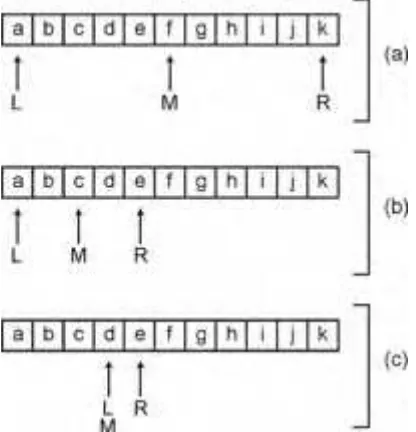
There might be other ways of finding “John Smith” in our hypothetical array. For example, if the array were sorted by last name, we could use thebinary searchalgorithm to find John Smith. We look at the middle element in the array. Is it John Smith? If so, we’re done. If it is less than John Smith (by “less than,” I mean earlier in alphabetic sequence), then we can assume that John Smith is in the first half of the array. If greater than, it’s in the latter half of the array. We can then do the same thing again, that is, look at the middle item and select the portion of the array that should have John Smith, slicing and dicing the array into smaller and smaller parts, until we either find it or the bit of the array we have left is empty.
Well, that algorithm certainly seems much more complicated than our origi-nal sequential search. The sequential search could be done with a nice simple For loop with a call to Break at the right moment; the code for the binary search would need a lot more calculations and local variables. So it might seem that sequential search is faster, just because it’s simpler to code.
2
TE
AM
FL
Y
Enter the world of algorithm analysis where we do experiments and try and formulate laws about how different algorithms actually work.
Analysis of Algorithms
Let’s look at the two possible searches for “John Smith” in an array: the sequential search and the binary search. We’ll implement both algorithms and then play with them in order to ascertain their performance attributes. Listing 1.1 is the simple sequential search.
Listing 1.1: Sequential search for a name in an array
function SeqSearch(aStrs : PStringArray; aCount : integer;
const aName : string5) : integer;
var
i : integer;
begin
for i := 0 to pred(aCount) do
if CompareText(aStrs^[i], aName) = 0 then begin
Result := i; Exit;
end; Result := -1;
end;
Listing 1.2 shows the more complex binary search. (At the present time we won’t go into what is happening in this routine—we discuss the binary search algorithm in detail in Chapter 4.)
Listing 1.2: Binary search for a name in an array
function BinarySearch(aStrs : PStringArray; aCount : integer;
const aName : string5) : integer;
var
L, R, M : integer; CompareResult : integer;
begin
L := 0;
R := pred(aCount);
while (L <= R) do begin
M := (L + R) div 2;
CompareResult := CompareText(aStrs^[M], aName);
if (CompareResult = 0) then begin
Result := M; Exit;
end
else if (CompareResult < 0) then
L := M + 1
R := M - 1;
end;
Result := -1;
end;
Just by looking at both routines it’s very hard to make a judgment about performance. In fact, this is a philosophy that we should embrace whole-heartedly: it can be very hard to tell how speed efficient some code is just by looking at it. Theonlyway we can truly find out how fast code is, is to run it. Nothing else will do. Whenever we have a choice between algorithms, as we do here, we shouldtestandtimethe code under different environments, with different inputs, in order to ascertain which algorithm is better for our needs.
The traditional way to do this timing is with aprofiler. The profiler program loads up our test application and then accurately times the various routines we’re interested in. My advice is to use a profiler as a matter of course in all your programming projects. It is only with a profiler that you can truly deter-mine where your application spends most of its time, and hence which routines are worth your spending time on optimization tasks.
The company I work for, TurboPower Software Company, has a professional profiler in its Sleuth QA Suite product. I’ve tested all of the code in this book under both StopWatch (the name of the profiling program in Sleuth QA Suite) and under CodeWatch (the resource and memory leak debugger in the suite). However, even if you do not have a profiler, you can still experiment and time routines; it’s just a little more awkward, since you have to embed calls to time routines in your code. Any profiler worth buying does not alter your code; it does its magic by modifying the executable in memory at run time.
For this experiment with searching algorithms, I wrote the test program to do its own timing. Essentially, the code grabs the system time at the start of the code being timed and gets it again at the end. From these two values it can calculate the time taken to perform the task. Actually, with modern faster machines and the low resolution of the PC clock, it’s usually beneficial to time several hundred calls to the routine, from which we can work out an average. (By the way, this program was written for 32-bit Delphi and will not compile with Delphi 1 since it allocates arrays on the heap that are greater than Delphi 1’s 64 KB limit.)
I ran the performance experiments in several different forms. First, I timed how long it took to find “Smith” in arrays containing 100, 1,000, 10,000, and 100,000 elements, using both algorithms and making sure that a “Smith” ele-ment was present. For the next series of tests, I timed how long it took to find
“Smith” in the same set of arrays with both algorithms, but this time I
ensured that “Smith” was not present. Table 1.1 shows the results of my tests. Table 1.1: Timing sequential and binary searches
Fail Success
Sequential
100 0.14 0.10
1,000 1.44 1.05
10,000 15.28 10.84
100,000 149.42 106.35
Binary
100 0.01 0.01
1,000 0.01 0.01
10,000 0.02 0.02
100,000 0.03 0.02
As you can see, the timings make for some very interesting reading. The time taken to perform a sequential search is proportional to the number of ele-ments in the array. We say that the execution characteristics of sequential search are linear.
However, the binary search statistics are somewhat more difficult to charac-terize. Indeed, it even seems as if we’re falling into a timing resolution problem because the algorithm is so fast. The relationship between the time taken and the number of elements in the array is no longer a simple linear one. It seems to be something much less than this, and something that is not brought out by these tests.
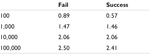
I reran the tests and scaled the binary timings by a factor of 100. Table 1.2: Retiming binary searches
Fail Success
100 0.89 0.57
1,000 1.47 1.46
10,000 2.06 2.06
100,000 2.50 2.41
by a constant amount (roughly half a unit). This is a logarithmic relationship: the time taken to do a binary search is proportional to the logarithm of the number of elements in the array.
(This can be a little hard to see for a non-mathematician. Recall from your school days that one way to multiply two numbers is to calculate their loga-rithms, add them, and then calculate the anti-logarithm to give the answer. Since we are multiplying by a factor of 10 in these profiling tests, it would be equivalent to adding a constant when viewed logarithmically. Exactly the case we see in the test results: we’re adding half a unit every time.)
So, what have we learned as a result of this experiment? As a first lesson, we have learned that the only way to understand the performance characteristics of an algorithm is to actually time it.
In general, the only way to see the efficiency of a piece of code is to time it. That applies to everything you write, whether you’re using a well-known algorithm or you’ve devised one to suit the current situation. Don’t guess, measure.
As a lesser lesson, we have also seen that sequential search is linear in nature, whereas binary search is logarithmic. If we were mathematically inclined, we could then take these statistical results and prove them as theorems. In this book, however, I do not want to overburden the text with a lot of mathemat-ics; there are plenty of college textbooks that could do it much better than I.
The Big-Oh Notation
We need a compact notation to express the performance characteristics we measure, rather than having to say things like “the performance of algorithm X is proportional to the number of items cubed,” or something equally ver-bose. Computer science already has such a scheme; it’s called the big-Oh notation.
For this notation, we work out the mathematical function ofn, the number of items, to which the algorithm’s performance is proportional, and say that the algorithm is a O(f(n)) algorithm, wheref(n) is some function ofn. We read this as “big-Oh off(n)”, or, less rigorously, as “proportional tof(n).”
For example, our experiments showed us that sequential search is a O(n) algorithm. Binary search, on the other hand, is a O(log(n)) algorithm. Since log(n) <n,for all positivenwe could say that binary search is always faster than sequential search; however, in a moment, I will give you a couple of warnings about taking conclusions from the big-Oh notation too far.
The big-Oh notation is succinct and compact. Suppose that by experimenta-tion we work out that algorithm X is O(n2+n); in other words, its
performance is proportional ton2+n. By “proportional to” we mean that we can find a constantksuch that the following equation holds true:
Performance =k* (n2+n)
Because of this equation, and others derived from the big-Oh notation, we can see firstly that multiplying the mathematical function inside the big-Oh parentheses by a constant value has no effect. For example, O(3*f(n)) is equal to O(f(n)); we can just take the “3” out of the notation and multiply it into the outside proportionality constant, the one we can conveniently ignore.
If the value ofnis large enough when we test algorithm X, we can safely say that the effects of the “+n” term are going to be swallowed up by then2 term. In other words, providednis large enough, O(n2+n) is equal to O(n2). And that goes for any additional term inn: we can safely ignore it if, for a sufficiently largen, its effects are swallowed by another term inn. So, for example, a term inn2will be swallowed up by a term inn3; a term in log(n) will be swallowed up by a term in n; and so on.
This shows that arithmetic with the big-Oh notation is very easy. Let’s, for argument’s sake, suppose that we have an algorithm that performs several different tasks. The first task, taken on its own, is O(n), the second is O(n2), the third is O(log(n)). What is the overall big-Oh value for the performance of the algorithm? The answer is O(n2), since that is the dominant part of the algorithm, by far.
Herein lies the warning I was about to give you before about drawing conclu-sions from big-Oh values. Big-Oh values are representative of what happens withlargevalues ofn. Forsmallvalues ofn, the notation breaks down com-pletely; other factors start to come into play and swamp the general results. For example, suppose we time two algorithms in an experiment. We manage to work out these two performance functions from our statistics:
Performance of first =k1* (n+ 100000) Performance of second =k2*n2
The two constantsk1andk2are of the same magnitude. Which algorithm would you use? If we went with the big-Oh notation, we’d always choose the first algorithm because it’s O(n). However, if we actually found that in our applicationsnwas never greater than 100, it would make more sense for us to use the second algorithm.
characteristics for the average number of items (or, if you like, the environ-ment) for which you will be using the algorithm. Again, the only way you’ll ever know you’ve selected the right algorithm is by measuring its speed in
yourapplication, foryourdata, with a profiler. Don’t take anything on trust from an author (like me, for example); measure, time, and test.
Best, Average, and Worst Cases
There’s another issue we need to consider as well. The big-Oh notation gener-ally refers to anaverage-casescenario. In our search experiment, if “Smith” were always the first item in the array, we’d find that sequential search would always be faster than binary search; we would succeed in finding the element we wanted after only one test. This is known as abest-casescenario and is O(1). (Big-Oh of 1 means that it takes a constant time, no matter how many items there are.)
If “Smith” were always the last item in the array, the sequential search would be pretty slow. This is aworst-casescenario and would be O(n), just like the average case.
Although binary search has a similar best-case scenario (the item we want is in the middle of the array), its worst-case scenario is still much better than that for sequential search. The performance statistics we gathered for the case where the element was not to be found in the array are all worst-case values.
In general, we should look at the big-Oh value for an algorithm’s average and worst cases. Best cases are usually not too interesting: we are generally more concerned with what happens “at the limit,” since that is how our applica-tions will be judged.
To conclude this particular section, we have seen that the big-Oh notation is a valuable tool for us to characterize various algorithms that do similar jobs. We have also discussed that the big-Oh notation is generally valid only for largen; for smallnwe are advised to take each algorithm and time it. Also, the only way for us to truly know how an algorithm will perform in our appli-cation is to time it. Don’t guess; use a profiler.
Algorithms and the Platform
Algorithms and the Platform
In all of this discussion about algorithms we didn’t concern ourselves with the operating system or the actual hardware on which the implementation of the algorithm was running. Indeed, the big-Oh notation could be said to only be valid for a fantasy machine, one where we can’t have any hardware or operat-ing system bottlenecks, for example. Unfortunately, we live and work in the
real world and our applications and algorithms will run on real physical machines, so we have to take these factors into account.
Virtual Memory and Paging
The first performance bottleneck we should understand is virtual memory paging. This is easier to understand with 32-bit applications, and, although 16-bit applications suffer from the same problems, the mechanics are slightly different. Note that I will only be talking in layman’s terms in this section: my intent is not to provide a complete discussion of the paging system used by your operating system, but just to provide enough information so that you conceptually understand what’s going on.
When we start an application on a modern 32-bit operating system, the sys-tem provides the application with a 4 GB virtual memory block for both code and data. It obviously doesn’tphysicallygive the application 4 GB of RAM to use (I don’t know about you, but I certainly do not have 4 GB of spare RAM for each application I simultaneously run); rather it provides a logical address space that, in theory, has 4 GB of memory behind it. This is virtual memory. It’s not really there, but, provided that we do things right, the oper-ating system will provide us with physical chunks of it that we can use when we need it.
The virtual memory is divided up intopages. On Win32 systems, using Pentium processors, the page size is 4 KB. Essentially, Win32 divides up the 4 GB virtual memory block into 4 KB pages and for each page it maintains a small amount of information about that page. (Linux’ memory system works in roughly the same manner.) The first piece of information is whether the page has beencommitted. A committed page is one where the application has stored some information, be it code or actual data. If a page is not committed, it is not there at all; any attempt to reference it will produce an access
violation.
The next piece of information is a mapping to a page translation table. In a typical system of 256 MB of memory (I’m very aware of how ridiculous that phrase will seem in only a few years’ time), there are only 65,536 physical pages available. The page translation table provides a mapping from a partic-ular virtual memory page as viewed by the application to an actual page available as RAM. So when we access a memory address in our application, some effort is going on behind the scenes to translate that address into a physical RAM address.
used and one of our applications wants to commit a new page. It can’t, since there’s no free RAM left. When this happens, the operating system writes a physical page out to disk (this is calledswapping) and marks that part of the translation table as being swapped out. The physical page is then remapped to provide a committed page for the requesting application.
This is all well and good until the application that owns the swapped out page actually tries to access it. The CPU notices that the physical page is no longer available and triggers apage fault. The operating system takes over, swaps another page to disk to free up a physical page, maps the requested page to the physical page, and then allows the application to continue. The application is totally unaware that this process has just happened; it just wanted to read the first byte of the page, for example, and that’s what (even-tually) happened.
All this magic occurs constantly as you use your 32-bit operating system. Physical pages are being swapped to and from disk and page mappings are being reset all the time. In general you wouldn’t notice it; however, in one particular situation, you will. That situation is known as thrashing.
Thrashing
When thrashing occurs, it can be deadly to your application, turning it from a highly tuned optimized program to a veritable sloth. Suppose you have an application that requires a lot of memory, say at least half the physical mem-ory in your machine. It creates a large array of large blocks, allocating them on the heap. This allocation will cause new pages to be committed, and, in all likelihood, for other pages to be swapped to disk. The program then reads the data in these large blocks in order from the beginning of the array to the end. The system has no problem swapping in required pages when necessary.
Suppose, now, that the application randomly looks at the blocks in the array. Say it refers to an address in block 56, followed by somewhere in block 123, followed by block 12, followed by block 234, and so on. In this scenario, it gets more and more likely that page faults will occur, causing more and more pages to be swapped to and from disk. Your disk drive light seems to blink very rapidly on and off and the program slows to a crawl. This is thrashing: the continual swapping of pages to disk to satisfy random requests from an application.
In general, there is little we can do about thrashing. The majority of the time we allocate our memory blocks from the Delphi heap manager. We have no control over where the memory blocks come from. It could be, for example, that related memory allocations all come from different pages. (ByrelatedI mean that the memory blocks are likely to be accessed at the same time
because they contain data that is related.) One way we can attempt to allevi-ate thrashing is to use separallevi-ate heaps for different structures and data in our application. This kind of algorithm is beyond the level of this book.
An example should make this clear. Suppose we have allocated a TList to con-tain some objects. Each of these objects concon-tains at least one string allocated on the heap (for example, we’re in 32-bit Delphi and the object uses long strings). Imagine now that the application has been running for a while and objects have been added and deleted from this TList. It’s not inconceivable that the TList instance, its objects, and the objects’ strings are spread out across many, many memory pages. If we then read the TList sequentially from start to finish, and access each object and its string(s), we will be touching each of these many pages, possibly resulting in many page swaps. If the num-ber of objects is fairly small, we probably would have most of the pages physically in memory anyway. But, if there were millions of objects in the TList, we might suffer from thrashing as we read through the list.
Locality of Reference
This brings up another concept:locality of reference. This principle is a way of thinking about our applications that helps us to minimize the possibility of thrashing. All this phrase means is that related pieces of information should be as close to each other in virtual memory as possible. If we have locality of reference, then when we access one item of data we should find other related items nearby in memory.
For example, an array of some record type has a high locality of reference. The element at index 1 is right next door in memory to the item at index 2, and so on. If we are sequentially accessing all the records in the array, we shall have an admirable locality of reference. Page swapping will be kept to a minimum. A TList instance containing pointers to the same record type— although it is still an array and can be said to have the same contents as the array of records—has low locality of reference. As we saw earlier, each of the items might be found on different pages, so sequentially accessing each item in the TList could presumably cause page swapping to occur. Linked lists (see Chapter 3) suffer from the same problems.
There are techniques to increase the locality of reference for various data structures and algorithms and we will touch on a few in this book. Unfortu-nately for us, the Delphi heap manager is designed to be as generic as
overriding the NewInstance class method, but we would have to do it with every class for which we need this capability.)
We have been talking about locality of reference in a spatial sense (“this object is close in memory to that object”), but we can also consider locality of reference in a temporal sense. This means that if an item has been referenced recently it will be referenced again soon, or that item X is always referenced at the same time as item Y. The embodiment of this temporal locality of refer-ence is a cache. A cacheis a small block of memory for some process that contains items that have recently been accessed. Every time an item is accessed the cache makes a copy of it in its own memory area. Once the memory area becomes full, the cache uses aleast recently used(LRU) algo-rithm to discard an item that hasn’t been referred to in a while to replace it with the most recently used item. That way the cache is maintaining a list of spatially local items that are also temporally local.
Normally, caches are used to store items that are held on slower devices, the classic example being a disk cache. However, in theory, a memory cache could work equally as well, especially in an application that uses a lot of memory and has the possibility to be run on a machine with not much RAM.
The CPU Cache
Indeed, the hardware on which we all program and run applications uses a memory cache. The machine on which I’m writing this chapter uses a 512 KB high-speed cache between the CPU and its registers and main memory (of which this machine has 192 MB). This high-speed cache acts as a buffer: when the CPU wants to read some memory, the cache will check to see if it has the memory already present and, if not, will go ahead and read it. Mem-ory that is frequently accessed—that is, has temporal locality of reference— will tend to stay in the cache.
Data Alignment
Another aspect of the hardware that we must take into account is that of data alignment. Current CPU hardware is built to always access data from the cache in 32-bit chunks. Not only that, but the chunks it requests are always
alignedon a 32-bit boundary. This means that the memory addresses passed to the cache from the CPU are always evenly divisible by four (4 bytes being 32 bits). It’s equivalent to the lower two bits of the address being clear. When 64-bit or larger CPUs become more prevalent, we’ll be used to the CPU
accessing 64 bits at a time (or 128 bits), aligned on the appropriate boundary.
12
TE
AM
FL
Y
So what does this have to do with our applications? Well, we have to make sure that our longint and pointer variables are also aligned on a 4-byte or 32-bit boundary. If they are not and they straddle a 4-byte boundary, the CPU has to issuetworeads to the cache, the first read to get the first part of the variable and the second read to get the second part. The CPU then stitches together the value from these two parts, throwing away the bytes it doesn’t need. (On other processors, the CPU actually enforces a rule that 32-bit enti-ties must be aligned on 32-bit boundaries. If not, you’ll get an access
violation. We’re lucky that Intel processors don’t enforce this rule, but then again, by not doing so it allows us to be sloppy.)
Always ensure that 32-bit entities are aligned on 32-bit boundaries and 16-bit entities on 16-bit boundaries. For slightly better efficiency, ensure that 64-bit entities (double variables, for example) are aligned on 64-bit boundaries.
This sounds complicated, but in reality, the Delphi compiler helps us an awful lot, and it is only in record type definitions that we have to be careful. All atomic variables (that is, of some simple type) that are global or local to a routine are automatically aligned properly. If we haven’t forced an alignment option with a compiler define, the 32-bit Delphi compiler will also automati-cally align fields in records properly. To do this it adds filler bytes to pad out the fields so that they align. With the 16-bit version, this automatic alignment in record types does not happen, so beware.
This automatic alignment feature sometimes confuses programmers. If we had the following record type in a 32-bit version of Delphi, what would sizeof(TMyRecord) return?
type
TMyRecord = record
aByte : byte; aLong : longint;
end;
Many people would say 5 bytes without thinking (and in fact this would be true in Delphi 1). The answer, though, is 8 bytes. The compiler will automati-cally add three bytes in between the aByte field and the aLong field, just so the latter can be forced onto a 4-byte boundary.
If, instead, we had declared the record type as (and notice the keyword packed),
type
TMyRecord = packed record
aByte : byte; aLong : longint;
then the sizeof function would indeed return 5 bytes. However, under this scheme, accessing the aLong field would take much longer than in the previ-ous type definition—it’s straddling a 4-byte boundary. So, the rule is, if you are going to use the packed keyword, you must arrange the fields in your record type definition to take account and advantage of alignment. Put all your 4-byte fields first and then add the other fields as required. I’ve followed this principle in the code in this book. And another rule is: never guess how big a record type is; use sizeof.
By the way, be aware that the Delphi heap manager also helps us out with alignment: all allocations from the heap manager are 4-byte aligned. Every pointer returned by GetMem or New has the lower two bits clear.
In Delphi 5 and above, the compiler goes even further. Not only does it align 4-byte entities on 4-byte boundaries, but it also aligns larger variables on 8-byte boundaries. This is of greatest importance for double variables: the FPU (floating-point unit) works better if double variables, being 8 bytes in size, are aligned on an 8-byte boundary. If your kind of programming is numeric intensive, make sure that your double fields in record structures are 8-byte aligned.
Space Versus Time Tradeoffs
The more we discover, devise, or analyze algorithms, the more we will come across what seems to be a universal computer science law: fast algorithms seem to have more memory requirements. That is, to use a faster algorithm we shall have to use more memory; to economize on memory might result in having to use a slower algorithm.
A simple example will explain the point I am trying to make. Suppose we wanted to devise an algorithm that counted the number of set bits in a byte value. Listing 1.3 is a first stab at an algorithm and hence a routine to do this.
Listing 1.3: Counting bits in a byte, original
function CountBits1(B : byte) : byte;
begin
Result := 0;
while (B<>0) do begin if Odd(B) then
inc(Result); B := B shr 1;
end;
end;
As you can see, this routine uses no ancillary storage at all. It merely counts the set bits by continually dividing the value by two (shifting an integer right by one bit is equal to dividing the integer by two), and counting the number of times an odd result is calculated. The loop stops when the value is zero, since at that point there are obviously no set bits left. The algorithm big-Oh value depends on the number of set bits in the parameter, and in a worst-case scenario the inner loop would have to be cycled through eight times. It is, therefore, a O(n) algorithm.
It seems like a pretty obvious routine and apart from some tinkering, such as rewriting it in Assembly language, there doesn’t seem to be any way to improve matters.
However, consider the requirement from another angle. The routine takes a 1-byte parameter, and there can be at most 256 different values passed through that parameter. So, why don’t we pre-compute all of the possible answers and store that in a static array in the application? Listing 1.4 shows this new algorithm.
Listing 1.4: Counting bits in a byte, improved
const
BitCounts : array [0..255] of byte =
(0, 1, 1, 2, 1, 2, 2, 3, 1, 2, 2, 3, 2, 3, 3, 4, 1, 2, 2, 3, 2, 3, 3, 4, 2, 3, 3, 4, 3, 4, 4, 5, 1, 2, 2, 3, 2, 3, 3, 4, 2, 3, 3, 4, 3, 4, 4, 5, 2, 3, 3, 4, 3, 4, 4, 5, 3, 4, 4, 5, 4, 5, 5, 6, 1, 2, 2, 3, 2, 3, 3, 4, 2, 3, 3, 4, 3, 4, 4, 5, 2, 3, 3, 4, 3, 4, 4, 5, 3, 4, 4, 5, 4, 5, 5, 6, 2, 3, 3, 4, 3, 4, 4, 5, 3, 4, 4, 5, 4, 5, 5, 6, 3, 4, 4, 5, 4, 5, 5, 6, 4, 5, 5, 6, 5, 6, 6, 7, 1, 2, 2, 3, 2, 3, 3, 4, 2, 3, 3, 4, 3, 4, 4, 5, 2, 3, 3, 4, 3, 4, 4, 5, 3, 4, 4, 5, 4, 5, 5, 6, 2, 3, 3, 4, 3, 4, 4, 5, 3, 4, 4, 5, 4, 5, 5, 6, 3, 4, 4, 5, 4, 5, 5, 6, 4, 5, 5, 6, 5, 6, 6, 7, 2, 3, 3, 4, 3, 4, 4, 5, 3, 4, 4, 5, 4, 5, 5, 6, 3, 4, 4, 5, 4, 5, 5, 6, 4, 5, 5, 6, 5, 6, 6, 7, 3, 4, 4, 5, 4, 5, 5, 6, 4, 5, 5, 6, 5, 6, 6, 7, 4, 5, 5, 6, 5, 6, 6, 7, 5, 6, 6, 7, 6, 7, 7, 8);
function CountBits2(B : byte) : byte;
begin
Result := BitCounts[B];
end;
algorithm calculates the number of bits in one simple step. (Note that I calcu-lated the static array automatically by writing a simple program using the first routine.)
On my machine, the second algorithm is 10 times faster than the first; you can call it 10 times in the same amount of time that a single call to the first one takes to execute. (Note, though, that I’m talking about the average-case scenario here—in the best-case scenario for the first routine, the parameter is zero and practically no code would be executed.)
So at the expense of a 256-byte array, we have devised an algorithm that is 10 times faster. We can trade speed for space with this particular need; we either have a fast routine and a large static array (which, it must be remem-bered, gets compiled into the executable program) or a slower routine without the memory extravagance. (There is another alternative: we could calculate the values in the array at run time, the first time the routine was called. This would mean that the array isn’t linked into the executable, but that the first call to the routine takes a relatively long time.)
This simple example is a graphic illustration of space versus time tradeoffs. Often we need to pre-calculate results in order to speed up algorithms, but this uses up more memory.
Long Strings
I cannot let a discussion on performance finish without talking a little about long strings. They have their own set of problems when you start talking about efficiency. Long strings were introduced in Delphi 2 and have appeared in all Delphi and Kylix compilers since that time (Delphi 1 programmers need not worry about them, nor this section).
A long string variable of type string is merely a pointer to a specially format-ted memory block. In other words, sizeof(stringvar) = sizeof(pointer). If this pointer is nil, the string is taken to be empty. Otherwise, the pointer points directly to the sequence of characters that makes up the string. The long string routines in the run-time library make sure that this sequence is always null terminated, hence you can easily typecast a string variable to a PChar for calls to the system API, for example. It is not generally well known that the memory block pointed to has some other information. The four bytes prior to the sequence of characters is an integer value containing the length of the string (less the null-terminator). The four bytes prior to that is an integer value with the reference count for the string (constant strings have this value set to –1). If the string is allocated on the heap, the four bytes prior to that is an integer value holding the complete size of the string memory block,
including all the hidden integer fields, the sequence of characters that make up the string, and the hidden null terminator, rounded up to the nearest four bytes.
The reference count is there so that code like: MyOtherString := MyString;
performs extremely quickly. The compiler converts this assignment to two separate steps: first, it increments the reference count for the string that MyString points to, and second it sets the MyOtherString pointer equal to the MyString pointer.
That’s about it for the efficiency gains. Everything else you do with strings will require memory allocations of one form or another.
Use const
If you pass a string into a routine and you don’t intend to alter it, then declare it with const. In most cases this will avoid the automatic addition of a hidden Try..finally block. If you don’t use const, the compiler assumes that you may be altering it and therefore sets up a local hidden string variable to hold the string. The reference count gets incremented at the beginning and will get decremented at the end. To ensure the latter happens, the compiler adds the hidden Try..finally block.
Listing 1.5 is a routine to count the number of vowels in a string.
Listing 1.5: Counting the number of vowels in a string
function CountVowels(const S : string) : integer;
var
i : integer;
begin
Result := 0;
for i := 1 to length(S) do
if upcase(S[i]) in [‘A’, ‘E’, ‘I’, ‘O’, ‘U’] then
inc(Result);
end;
If the keyword const is removed from the function statement, the speed of the routine is reduced by about 12 percent, the cost of the hidden Try..finally block.
Be Wary of Automatic Conversions
what is really going on. Take the Pos function, for example. As you know, this function returns the position of a substring in a larger string. If you use it for finding a character:
PosOfCh := Pos(SomeChar, MyString);
you need to be aware that the compiler will convert the character into a long string. It will allocate a long string on the heap, make it length 1 and copy the character into it. It then calls the Pos function. Because there is an automatic hidden string being used, a hidden Try..finally block is included to free the one-character string at the end of the routine. The routine in Listing 1.6 isfive
times faster (yes, five!), despite it being written in Pascal and not assembler.
Listing 1.6: Position of a character in a string
function TDPosCh(aCh : AnsiChar; const S : string) : integer;
var
i : integer;
begin
Result := 0;
for i := 1 to length(S) do if (S[i] = aCh) then begin
Result := i; Exit;
end;
end;
My recommendation is to check the syntax of routines you are calling with a character to make sure that the parameter concerned is really a character and not a string.
There’s another wrinkle to this hint. The string concatentation operator, +, also acts on strings only. If you are appending a character to a string in a loop, try and find another way to do it (say by presetting the length of the string and then making assignments to the individual characters in the string) since again the compiler will be converting all the characters to strings
behind your back.
Debugging and Testing
Debugging and Testing
Let’s put aside our discussions of algorithmic performance now and talk a lit-tle about procedural algorithms—algorithms for performing the development process, not for calculating a result.
No matter how we write our code, at some point we must test it to make sure that it performs in the manner we intended. For a certain set of input values, do we get the expected result? If we click on the OK button, is the record
saved to the database? Of course, if a test we perform fails, we need to try and work out why it failed and fix the problem. This is known as debug-ging—the test revealed a bug and now we need to remove that bug. Testing and debugging are therefore inextricably linked; they are the two faces of the same coin.
Given that we cannot get away with not testing (we like to think of ourselves as infallible and our code as perfect, but unfortunately this isn’t so), what can we do to make it easier for ourselves?
The first golden rule is this:Code we write will always contain bugs.There is no moral angle to this rule; there is nothing of which to be ashamed. Buggy code is part of our normal daily lives as programmers. Like it or not, we pro-grammers are fallible. No matter how hard we try we’ll introduce at least one bug when developing. Indeed, part of the fun of programming, I find, is find-ing that particularly elusive bug and nailfind-ing it.
Rule 1: Code we write will always contain bugs.
Although I said that there is nothing to be embarrassed about if some of your code is discovered to have a bug, there is one situation where it does reflect badly on you—that is when you didn’t test adequately.
Assertions
Since the first rule indicates that we will always have to do some debugging, and the corollary states that we don’t want to be embarrassed by inade-quately tested code, we need to learn to program defensively. The first tool in our defensive arsenal is theassertion.
An assertion is a programmatic check in the code to test whether a particular condition is true. If the condition is false, contrary to your expectation, an exception is raised and you get a nice dialog box explaining the problem. This dialog box is a signal warning you that either your supposition was wrong, or the code is being used in a way you hadn’t foreseen. The assertion exception should lead you directly to that part of the code that has the bug. Assertions are a key element of defensive programming: when you add an assertion into your code, you are stating unequivocally that something must be true before continuing past that point.
Rule 2: Assert early, assert often.
Unfortunately, some Delphi programmers will have a problem with this. Com-piler-supported assertions didn’t arrive until Delphi 3. From that moment, programmers could use assertions with impunity. We were given a compiler option that either compiled in the assertion checks into the executable or magically ignored them. For testing and debugging, we would compile with assertions enabled. For a production build, we would disable them and they would not appear in the compiled code.
For Delphi 1 and Delphi 2, we therefore have to do something else. There are two solutions. The first is to write a method called Assert whose implementa-tion is empty when we do a producimplementa-tion build, and has a check of the
condition together with a call to Raise if not. Listing 1.7 shows this simple assertion procedure.
Listing 1.7: The assertion procedure for Delphi 1 and 2
procedure Assert(aCondition : boolean; const aFailMsg : string);
begin
{$IFDEF UseAssert}
if not aCondition then
raise Exception.Create(aFailMsg); {$ENDIF}
end;
As you can see, we use a compiler define to either compile in the assertion check or to remove it. Although this procedure is simple to use and is fairly easy to call from our main code, it does mean that in a production build there is a call to an empty procedure wherever we code an assertion. The alterna-tive is to move the $IFDEF out of this procedure to wherever we call Assert. Statement blocks would then invade our code in the following manner: ...
{$IFDEF UseAssert}
Assert(MyPointer<>nil, ‘MyPointer should be allocated by now’); {$ENDIF}
MyPointer^.Field := 0; ...
The benefit of this organization is that the calls to the Assert procedure disap-pear completely in a production build, when the UseAssert compiler define is not defined. Since the code for this book is designed to be compiled with all versions of Delphi, I use the Assert procedure shown in Listing 1.7.
There are three ways to use an assertion: pre-conditions, post-conditions, and invariants. Apre-conditionis an assertion you place at the beginning of a
routine. It states unequivocally what should be true about the program