Thermodynamic Models
for Industrial Applications
From Classical and Advanced
Mixing Rules to Association Theories
GEORGIOS M. KONTOGEORGIS Technical University of Denmark, Lyngby, Denmark
Thermodynamic Models
for Industrial Applications
From Classical and Advanced
Mixing Rules to Association Theories
GEORGIOS M. KONTOGEORGIS Technical University of Denmark, Lyngby, Denmark
Registered office
John Wiley & Sons Ltd, The Atrium, Southern Gate, Chichester, West Sussex, PO19 8SQ, United Kingdom For details of our global editorial offices, for customer services and for information about how to apply for permission to reuse the copyright material in this book please see our website at www.wiley.com .
The right of the author to be identified as the author of this work has been asserted in accordance with the Copyright, Designs and Patents Act 1988.
All rights reserved. No part of this publication may be reproduced, stored in a retrieval system, or transmitted, in any form or by any means, electronic, mechanical, photocopying, recording or otherwise, except as permitted by the UK Copyright, Designs and Patents Act 1988, without the prior permission of the publisher.
Wiley also publishes its books in a variety of electronic formats. Some content that appears in print may not be available in electronic books.
Designations used by companies to distinguish their products are often claimed as trademarks. All brand names and product names used in this book are trade names, service marks, trademarks or registered trademarks of their respective owners. The publisher is not associated with any product or vendor mentioned in this book. This publication is designed to provide accurate and authoritative information in regard to the subject matter covered. It is sold on the understanding that the publisher is not engaged in rendering professional services. If professional advice or other expert assistance is required, the services of a competent professional should be sought.
The publisher and the author make no representations or warranties with respect to the accuracy or completeness of the contents of this work and specifically disclaim all warranties, including without limitation any implied warranties of fitness for a particular purpose. This work is sold with the understanding that the publisher is not engaged in rendering professional services. The advice and strategies contained herein may not be suitable for every situation. In view of ongoing research, equipment modifications, changes in governmental regulations, and the constant flow of information relating to the use of experimental reagents, equipment, and devices, the reader is urged to review and evaluate the information provided in the package insert or instructions for each chemical, piece of equipment, reagent, or device for, among other things,
any changes in the instructions or indication of usage and for added warnings and precautions. The fact that an organization or Website is referred to in this work as a citation and/or a potential source of further information does not mean that the author or the publisher endorses the information the organization or Website may provide or recommendations it may make. Further, readers should be aware that Internet Websites listed in this work may have changed or disappeared between when this work was written and when it is read. No warranty may be created or extended by any promotional statements for this work. Neither the publisher nor the author shall be liable for any damages arising herefrom.
Library of Congress Cataloging-in-Publication Data
Kontogeorgis, Georgios M.
Thermodynamic models for industrial applications : from classical and advanced mixing rules to association theories / Georgios M. Kontogeorgis, Georgios K. Folas.
p. cm.
Includes bibliographical references and index. ISBN 978-0-470-69726-9 (cloth)
1. Thermodynamics–Industrial applications. 2. Chemical engineering. I. Kontogeorgis, Georgios M. II. Folas, Georgios K. III. Title.
TP155.2.T45K66 2010 660’.2969–dc22
2009028762 A catalogue record for this book is available from the British Library. ISBN: 978-0-470-69726-9 (Cloth)
Set in 10/12 pt, Times Roman by Thomson Digital, Noida, India
Our families especially (in Denmark, The Netherlands and Greece)
have deeply felt the consequences of the process of writing this book.
I (Georgios Kontogeorgis) would like to dedicate the book to my wife
Olga for her patience, support, love and understanding – especially as,
during the period of writing of this book, our daughter,
Elena, was born.
I (Georgios Folas) would like to thank Georgios Kontogeorgis for
our excellent collaboration in writing this monograph during the past
two years. I am grateful to my family and wish to dedicate this book to
Contents
Preface xvii
About the Authors xix
Acknowledgments xxi
List of Abbreviations xxiii
List of Symbols xxvii
PART A INTRODUCTION 1
1 Thermodynamics for process and product design 3
Appendix 9
References 14
2 Intermolecular forces and thermodynamic models 17
2.1 General 17
2.1.1 Microscopic (London) approach 21
2.1.2 Macroscopic (Lifshitz) approach 22
2.2 Coulombic and van der Waals forces 22
2.3 Quasi-chemical forces with emphasis on hydrogen bonding 26
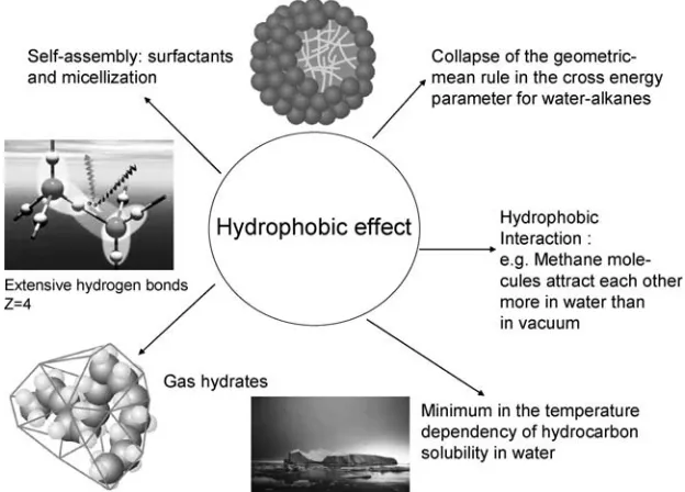
2.3.1 Hydrogen bonding and the hydrophobic effect 26
2.3.2 Hydrogen bonding and phase behavior 29
2.4 Some applications of intermolecular forces
in model development 30
2.4.1 Improved terms in equations of state 31
2.4.2 Combining rules in equations of state 32
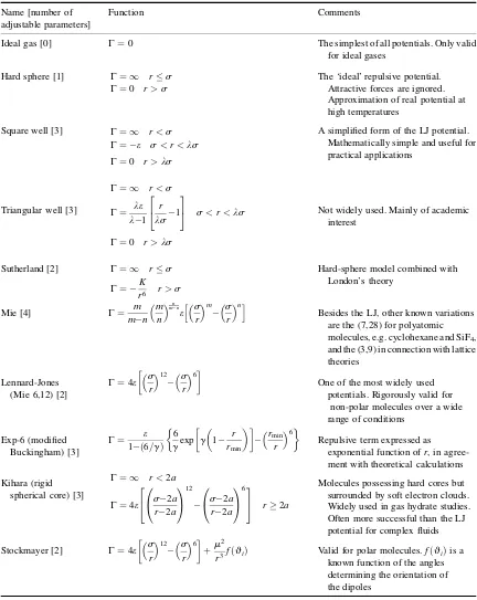
2.4.3 Beyond the Lennard-Jones potential 33
2.4.4 Mixing rules 34
2.5 Concluding remarks 36
References 36
PART B THE CLASSICAL MODELS 39
3 Cubic equations of state: the classical mixing rules 41
3.1 General 41
3.2 On parameter estimation 45
3.2.1 Pure compounds 45
3.3 Analysis of the advantages and shortcomings of cubic EoS 51
3.3.1 Advantages of Cubic EoS 51
3.3.2 Shortcomings and limitations of cubic EoS 52
3.4 Some recent developments with cubic EoS 58
3.4.1 Use of liquid densities in the EoS parameter estimation 59
3.4.2 Activity coefficients for evaluating mixing and combining rules 61
3.4.3 Mixing and combining rules – beyond the vdW1f and classical
combining rules 65
3.5 Concluding remarks 67
Appendix 68
References 74
4 Activity coefficient models Part 1: random-mixing models 79
4.1 Introduction to the random-mixing models 79
4.2 Experimental activity coefficients 80
4.2.1 VLE 80
4.2.2 SLE (assuming pure solid phase) 80
4.2.3 Trends of the activity coefficients 81
4.3 The Margules equations 82
4.4 From the van der Waals and van Laar equation to the
regular solution theory 84
4.4.1 From the van der Waals EoS to the van Laar model 84
4.4.2 From the van Laar model to the Regular Solution Theory (RST) 86
4.5 Applications of the Regular Solution Theory 88
4.5.1 General 88
4.5.2 Low-pressure VLE 89
4.5.3 SLE 90
4.5.4 Gas-Liquid equilibrium (GLE) 91
4.5.5 Polymers 92
4.6 SLE with emphasis on wax formation 97
4.7 Asphaltene precipitation 99
4.8 Concluding remarks about the random-mixing-based models 100
Appendix 104
References 106
5 Activity coefficient models Part 2: local composition models, from
Wilson and NRTL to UNIQUAC and UNIFAC 109
5.1 General 109
5.2 Overview of the local composition models 110
5.2.1 NRTL 110
5.2.2 UNIQUAC 112
5.2.3 On UNIQUAC’s energy parameters 113
5.2.4 On the Wilson equation parameters 114
5.3 The theoretical limitations 114
5.3.1 Necessity for three models 116
5.5 On the theoretical significance of the interaction parameters 123
5.5.1 Parameter values for families of compounds 123
5.5.2 One-parameter LC models 123
5.5.3 Comparison of LC model parameters to quantum chemistry
and other theoretically determined values 126
5.6 LC Models: some unifying concepts 126
5.6.1 Wilson and UNIQUAC 127
5.6.2 The interaction parameters of the LC models 128
5.6.3 Successes and limitations of the LC models 128
5.7 The group contribution principle and UNIFAC 129
5.7.1 Why there are so many UNIFAC variants 133
5.7.2 UNIFAC applications 134
5.8 Local-compositon-free–volume models for polymers 135
5.8.1 Introduction 135
5.8.2 FV non-random-mixing models 137
5.9 Conclusions: is UNIQUAC the best local compostion model available today? 140
Appendix 147
References 154
6 The EoS/GEmixing rules for cubic equations of state 159
6.1 General 159
6.2 The infinite pressure limit (the Huron–Vidal mixing rule) 161
6.3 The zero reference pressure limit (the Michelsen approach) 163
6.4 Successes and limitations of zero reference pressure models 165
6.5 The Wong–Sandler (WS) mixing rule 167
6.6 EoS/GEapproaches suitable for asymmetric mixtures 168
6.7 Applications of the LCVM, MHV2, PSRK and WS mixing rules 174
6.8 Cubic EoS for polymers 181
6.8.1 High-pressure polymer thermodynamics 181
6.8.2 A simple first approach: application of the vdW EoS to polymers 182
6.8.3 Cubic EoS for polymers 184
6.8.4 How to estimate EoS parameters for polymers 187
6.9 Conclusions: achievements and limitations of the EoS/GEmodels 187
6.10 Recommended Models – so far 189
Appendix 189
References 190
PART C ADVANCED MODELS AND THEIR APPLICATIONS 195
7 Association theories and models: the role of spectroscopy 197
7.1 Introduction 197
7.2 Three different association theories 197
7.3 The chemical and perturbation theories 198
7.3.1 Introductory thoughts: the separability of terms in chemical-based EoS 198
7.3.2 Beyond oligomers and beyond pure compounds 200
7.3.3 Extension to mixtures 201
7.4 Spectroscopy and association theories 202
7.4.1 A key property 202
7.4.2 Similarity between association theories 204
7.4.3 Use of the similarities between the various association theories 206
7.4.4 Spectroscopic data and validation of theories 207
7.5 Concluding remarks 213
Appendix 214
References 218
8 The Statistical Associating Fluid Theory (SAFT) 221
8.1 The SAFT EoS: a brief look at the history and major developments 221
8.2 The SAFT equations 225
8.2.1 The chain and association terms 225
8.2.2 The dispersion terms 227
8.3 Parameterization of SAFT 233
8.3.1 Pure compounds 233
8.3.2 Mixtures 239
8.4 Applications of SAFT to non-polar molecules 241
8.5 GC SAFT approaches 245
8.5.1 French method 245
8.5.2 DTU method 246
8.5.3 Other methods 247
8.6 Concluding remarks 248
Appendix 249
References 256
9 The Cubic-Plus-Association equation of state 261
9.1 Introduction 261
9.1.1 The importance of associating (hydrogen bonding) mixtures 261
9.1.2 Why specifically develop the CPA EoS? 262
9.2 The CPA EoS 263
9.2.1 General 263
9.2.2 Mixing and combining rules 264
9.3 Parameter estimation: pure compounds 265
9.3.1 Testing of pure compound parameters 266
9.4 The First applications 272
9.4.1 VLE, LLE and SLE for alcohol–hydrocarbons 272
9.4.2 Water–hydrocarbon phase equilibria 273
9.4.3 Water–methanol and alcohol–alcohol phase equilibria 276
9.4.4 Water–methanol–hydrocarbons VLLE: prediction of methanol
partition coefficient 279
9.5 Conclusions 283
Appendix 284
References 296
10 Applications of CPA to the oil and gas industry 299
10.2 Glycol–water–hydrocarbon phase equilibria 300
10.2.1 Glycol–hydrocarbons 300
10.2.2 Glycol–water and multicomponent mixtures 303
10.3 Gas hydrates 306
10.3.1 General 306
10.3.2 Thermodynamic framework 307
10.3.3 Calculation of hydrate equilibria 308
10.3.4 Discussion 312
10.4 Gas phase water content calculations 315
10.5 Mixtures with acid gases (CO2and H2S) 316
10.6 Reservoir fluids 323
10.6.1 Heptanes plus characterization 324
10.6.2 Applications of CPA to reservoir fluids 325
10.7 Conclusions 329
References 329
11 Applications of CPA to chemical industries 333
11.1 Introduction 333
11.2 Aqueous mixtures with heavy alcohols 334
11.3 Amines and ketones 336
11.3.1 The case of a strongly solvating mixture: acetone–chloroform 338
11.4 Mixtures with organic acids 341
11.5 Mixtures with ethers and esters 348
11.6 Multifunctional chemicals: glycolethers and alkanolamines 352
11.7 Complex aqueous mixtures 357
11.8 Concluding remarks 361
Appendix 364
References 366
12 Extension of CPA and SAFT to new systems: worked examples and guidelines 369
12.1 Introduction 369
12.2 The Case of sulfolane: CPA application 370
12.2.1 Introduction 370
12.2.2 Sulfolane: is it an ‘inert’ (non-self-associating) compound? 370
12.2.3 Sulfolane as a self-associating compound 374
12.3 Application of sPC–SAFT to sulfolane-related systems 379
12.4 Applicability of association theories and cubic EoS with advanced mixing
rules (EoS/GEmodels) to polar chemicals 381
12.5 Phenols 383
12.6 Conclusions 387
References 387
13 Applications of SAFT to polar and associating mixtures 389
13.1 Introduction 389
13.2 Water–hydrocarbons 389
13.3 Alcohols, amines and alkanolamines 395
13.3.2 Discussion 396
13.3.3 Study of alcohols with generalized associating parameters 401
13.4 Glycols 402
13.5 Organic acids 403
13.6 Polar non-associating compounds 404
13.6.1 Theories for extension of SAFT to polar fluids 405
13.6.2 Application of the tPC–PSAFT EoS to complex polar fluid mixtures 409
13.6.3 Discussion: comparisons between various polar SAFT EoS 413
13.6.4 The importance of solvation (induced association) 419
13.7 Flow assurance (asphaltenes and gas hydrate inhibitors) 422
13.8 Concluding remarks 424
References 425
14 Application of SAFT to polymers 429
14.1 Overview 429
14.2 Estimation of polymer parameters for SAFT-type EoS 429
14.2.1 Estimation of polymer parameters for EoS: general 429
14.2.2 The Kouskoumvekakiet al. method 431
14.2.3 Polar and associating polymers 435
14.2.4 Parameters for co-polymers 438
14.3 Low-pressure phase equilibria (VLE and LLE) using
simplified PC–SAFT 439
14.4 High-pressure phase equilibria 447
14.5 Co-polymers 450
14.6 Concluding remarks 451
Appendix 454
References 458
PART D THERMODYNAMICS AND OTHER DISCIPLINES 461
15 Models for electrolyte systems 463
15.1 Introduction: importance of electrolyte mixtures and modeling challenges 463
15.1.1 Importance of electrolyte systems and coulombic forces 463
15.1.2 Electroneutrality 464
15.1.3 Standard states 464
15.1.4 Mean ionic activity coefficients (of salts) 466
15.1.5 Osmotic activity coefficients 467
15.1.6 Salt solubility 468
15.2 Theories of ionic (long-range) interactions 468
15.2.1 Debye–H€uckel vs. mean spherical approximation 468
15.2.2 Other ionic contributions 472
15.2.3 The role of the dielectric constant 473
15.3 Electrolyte models: activity coefficients 473
15.3.1 Introduction 473
15.3.2 Comparison of models 476
15.4 Electrolyte models: Equation of State 483
15.4.1 General 483
15.4.2 Lewis–Randall vs. McMillan–Mayer framework 486
15.5 Comparison of electrolyte EoS: capabilities and limitations 486
15.5.1 Cubic EoSþelectrolyte terms 486
15.5.2 e-CPA EoS 488
15.5.3 e-SAFT EoS 492
15.5.4 Ionic liquids 500
15.6 Thermodynamic models for CO2–water–alkanolamines 500
15.6.1 Introduction 500
15.6.2 The Gabrielsen model 505
15.6.3 Activity coefficient models (g wapproaches) 507
15.6.4 Equation of State 512
15.7 Concluding remarks 519
References 520
16 Quantum chemistry in engineering thermodynamics 525
16.1 Introduction 525
16.2 The COSMO–RS method 527
16.2.1 Introduction 527
16.2.2 Range of applicability 527
16.2.3 Limitations 528
16.3 Estimation of association model parameters using QC 531
16.4 Estimation of size parameters of SAFT-type models from QC 540
16.4.1 The approach of Imperial College 540
16.4.2 The approach of Aachen 542
16.5 Conclusions 547
References 547
17 Environmental thermodynamics 551
17.1 Introduction 551
17.2 Distribution of chemicals in environmental ecosystems 552
17.2.1 Scope and importance of thermodynamics in environmental calculations 552
17.2.2 Introduction to the key concepts of environmental thermodynamics 557
17.2.3 Basic relationships of environmental thermodynamics 559
17.2.4 The octanol–water partition coefficient 566
17.3 Environmentally friendly solvents: supercritical fluids 572
17.4 Conclusions 573
References 574
18 Thermodynamics and colloid and surface chemistry 577
18.1 General 577
18.2 Intermolecular vs. interparticle forces 577
18.2.1 Intermolecular forces and theories for interfacial tension 577
18.2.2 Characterization of solid interfaces with interfacial tension theories 582
18.3 Interparticle forces in colloids and interfaces 585
18.3.1 Interparticle forces and colloids 585
18.3.2 Forces and colloid stability 587
18.3.3 Interparticle forces and adhesion 590
18.4 Acid–base concepts in adhesion studies 591
18.4.1 Adhesion measurements and interfacial forces 591
18.4.2 Industrial examples 593
18.5 Surface and interfacial tensions from thermodynamic models 594
18.5.1 The gradient theory 594
18.6 Hydrophilicity 597
18.6.1 The CPP parameter 598
18.6.2 The HLB parameter 598
18.7 Micellization and surfactant solutions 600
18.7.1 General 600
18.7.2 CMC, Krafft point and micellization 601
18.7.3 CMC estimation from thermodynamic models 602
18.8 Adsorption 604
18.8.1 General 604
18.8.2 Some applications of adsorption 605
18.8.3 Multicomponent Langmuir adsorption and the vdW–Platteeuw
solid solution theory 608
18.9 Conclusions 609
References 610
19 Thermodynamics for biotechnology 613
19.1 Introduction 613
19.2 Models for Pharmaceuticals 613
19.2.1 General 613
19.2.2 The NRTL–SAC model 615
19.2.3 The NRHB model for pharmaceuticals 618
19.3 Models for amino acids and polypeptides 619
19.3.1 Chemistry and basic relationships 619
19.3.2 The excess solubility approach 624
19.3.3 Classical modeling approaches 624
19.3.4 Modern approaches 627
19.4 Adsorption of proteins and chromatography 631
19.4.1 Introduction 631
19.4.2 Fundamentals of adsorption related to two chromatographic separations 631
19.4.3 A simple adsorption model (low protein concentrations) 633
19.4.4 Discussion 635
19.5 Semi-predictive models for protein systems 637
19.5.1 The osmotic second virial coefficient and protein solubility: a
tool for modeling protein precipitation 638
19.5.2 Partition coefficients in protein–micelle systems 639
19.5.3 Partition coefficients in aqueous two-phase systems
19.6 Concluding Remarks 644
Appendix 644
References 652
20 Epilogue: thermodynamic challenges in the twenty-first century 655
20.1 In brief 655
20.2 Petroleum and chemical industries 656
20.3 Chemicals including polymers and complex product design 658
20.4 Biotechnology including pharmaceuticals 659
20.5 How future needs will be addressed 660
References 661
Preface
Thermodynamics plays an important role in numerous industries, both in the design of separation equipment and processes as well as for product design and optimizing formulations. Complex polar and associating molecules are present in many applications, for which different types of phase equilibria and other thermodynamic properties need to be known over wide ranges of temperature and pressure. Several applications also include electrolytes, polymers or biomolecules. To some extent, traditional activity coefficient models are being phased out, possibly with the exception of UNIFAC, due to its predictive character, as advances in computers and statistical mechanics favor use of equations of state. However, some of these ‘classical’ models continue to find applications, especially in the chemical, polymer and pharmaceutical industries. On the other hand, while traditional cubic equations of state are often not adequate for complex phase equilibria, over the past 20–30 years advanced thermodynamic models, especially equations of state, have been developed.
The purpose of this work is to present and discuss in depth both ‘classical’ and novel thermodynamic models which have found or can potentially be used for industrial applications. Following the first introductory part of two short chapters on the fundamentals of thermodynamics and intermolecular forces, the second part of the book (Chapters 3–6) presents the ‘classical’ models, such as cubic equations of state, activity coefficient models and their combination in the so-called EoS/GEmixing rules. The advantages, major applications and reliability are discussed as well as the limitations and points of caution when these models are used for design purposes, typically within a commercial simulation package. Applications in the oil and gas and chemical sectors are emphasized but models suitable for polymers are also presented in Chapters 4–6.
The third part of the book (Chapters 7–14) presents several of the advanced models in the form of association equations of state which have been developed since the early 1990s and are suitable for industrial applications. While many of the principles and applications are common to a large family of these models, we have focused on two of the models (the CPA and PC–SAFT equations of state), largely due to their range of applicability and our familiarity with them. Extensive parameter tables for the two models are available in the two appendices on the companion website at www.wiley.com/go/Kontogeorgis. The final part of the book (Chapters 15–20) illustrates applications of thermodynamics in environmental science and colloid and surface chemistry and discusses models for mixtures containing electrolytes. Finally, brief introductions about the thermodynamic tools available for mixtures with biomolecules as well as the possibility of using quantum chemistry in engineering thermodynamics conclude the book.
The book is based on our extensive experience of working with thermodynamic models, especially the association equations of state, and in close collaboration with industry in the petroleum, energy, chemical and polymer sectors. While we feel that we have included several of the exciting developments in thermodynamic models with an industrial flavor, it has not been possible to include them all. We would like, therefore, to apologize in advance to colleagues and researchers worldwide whose contributions may not have been included or adequately discussed for reasons of economy. However, we are looking forward to receiving comments and suggestions which can lead to improvements in the future.
graduate courses on applied chemical engineering thermodynamics, provided that a course on the funda-mentals of applied thermodynamics has been previously followed. For this reason, problems are provided on the companion website at www.wiley.com/go/Kontogeorgis. Answers to selected problems are available, while a full solution manual is available from the authors.
Georgios M. Kontogeorgis Copenhagen, Denmark
About the Authors
Georgios M. Kontogeorgis has been a professor at the Technical University of Denmark (DTU), Department of Chemical and Biochemical Engineering, since January 2008. Prior to that he was associate professor at the same university, a position he had held since August 1999. He has an MSc in Chemical Engineering from the Technical University of Athens (1991) and a PhD from DTU (1995). His current research areas are energy (especially thermodynamic models for the oil and gas industry), materials and nanotechnol-ogy (especially polymers – paints, product design, and colloid and surface chemistry), environment (design CO2capture units, fate of chemicals, migration of plasticizers) and biotechnology. He is the author of over 100
publications in international journals and co-editor of one monograph. He is the recipient of the Empirikion Foundation Award for ‘Achievements in Chemistry’ (1999, Greece) and of the Dana Lim Price (2002, Denmark).
Acknowledgments
We wish to thank all our students and colleagues and especially the faculty members of IVC-SEP Research Center, at the Department of Chemical and Biochemical Engineering of the Technical University of Denmark (DTU), for the many inspiring discussions during the past 10 years which have largely contributed to the shaping of this book. Our very special thanks go to Professor Michael L. Michelsen for the endless discussions we have enjoyed with him on thermodynamics.
In the preparation of this book we have been assisted by many colleagues, friends, current and former students. Some have read chapters of the book or provided material prior to publication, while we have had extensive discussions with others. We would particularly like to thank Professors J. Coutinho, G. Jackson, I. Marrucho, J. Mollerup, G. Sadowski, L. Vega and N. von Solms, Doctors M. Breil, H. Cheng, Ph. Coutsikos, J.-C. de Hemptinne, I. Economou, J. Gabrielsen, A. Grenner, E. Karakatsani I. Kouskoumvekaki, Th. Lindvig, E. Solbraa, N. Sune, A. Tihic, I. Tsivintzelis and W. Yan, as well as the current PhD and MSc students of IVC-SEP, namely A. Avlund, J. Christensen, L. Faramarzi, F. Leon, B. Maribo-Mogensen and A. Sattar-Dar.
List of Abbreviations
AAD % percentage average absolute deviation:
AAD %¼ 1
NP
XNP
i¼1
ABS xexp;i xcalc;i xexp;i
100
for a propertyx
AM arithmetic mean rule (for the cross co-volume parameter,b12)
AMP 2-amino-2-methyl-1-propanol
ATPS aqueous two-phase systems
BCF bioconcentration factor
BR butadiene rubber (polybutadiene)
BTEX benzene–toluene–ethylbenzene–xylene
CCC critical coagulation concentration
CDI chronic daily intake
CK–SAFT Chen–Kreglewski SAFT
CMC critical micelle concentration
Comb-FV combinatorial free volume (effect, term, contributions)
COSMO conductor-like screening model
CPA cubic-plus-association
CPP critical packing parameter
CS Carnahan–Starling
CSP corresponding states principle
CTAB hexadecyl trimethylammonium bromide
DBE dibutyl ether
DDT dichlorodiphenyltrichloroethane
DEA diethanolamine
DEG diethylene glycol
DFT density functional theory
DH Debye–H€uckel
DiPE diisopropyl ether
DIPPR Design Institute for Physical Property (database)
DLVO Derjaguin–Landau–Verwey–Overbeek (theory)
DME dimethyl ether
DPE dipropyl ether
ECR Elliott’s combining rule
EoS Equation of state
EPA Environmental Protection Agency
EPE ethyl propyl ether
ESD Elliott–Suresh–Donohue (EoS)
EU European Union
FH Flory–Huggins
FOG first-order groups
FV Free volume
GC group contribution (methods, principle)
GCA group contribution plus association
GCVM group contribution of Vidal and Michelsen mixing rules
GERG Group Europeen de Recherche Gaziere
GLC gas–liquid chromatography
GLE gas–liquid equilibria
GM geometric mean rule (for the cross-energy parameter,a12)
HB hydrogen bonds/bonding
HCB hexachlorobenzene
HF Hartree–Fock
HIC hydrophobic interaction chromatography
HLB hydrophilic–lipophilic balance
HSP Hansen solubility parameters
HV Huron–Vidal mixing rule
IEC ion-exchange chromatography
LALS low-angle light scattering
LC local composition (models, principle, etc.)
LCST lower critical solution temperature
LCVM linear combination of Vidal and Michelsen mixing rules
LGT linear gradient theory
LJ Lennard-Jones
LLE liquid–liquid equilibria
LR Lewis–Randall; long range
mCR-1 modified CR-1 combining rule (for the CPA EoS), equation (9.10)
MC–SRK Mathias–Copeman SRK
MDEA methyl diethanolamine
MEA monoethanolamine
MEG (mono)ethylene glycol
MEK methyl ethyl ketone
MHV1 modified Huron–Vidal first order
MHV2 modified Huron–Vidal second order
MM McMillan–Mayer
MO molecular orbital
MSA mean spherical approximation
MW molecular weight
NLF–HB lattice–fluid hydrogen bonding (EoS)
NP number of experimental points
NRHB non-random hydrogen bonding (EoS)
NRTL non-random two liquid
PAHs polynuclear aromatic hydrocarbons
PBA poly(butyl acrylate)
PBD polybutadiene
PBMA poly(butyl methacrylate)
PC–SAFT perturbed-chain SAFT
PDH Pitzer–Debye–H€uckel
PDMS poly(dimethyl siloxane)
PEA poly(ethyl acrylate)
PEG (poly)ethylene glycol
PIB polyisobutylene
PIPMA poly(isopropyl methacrylate)
PM primitive model
PMA poly(methyl acrylate)
PMMA poly(methyl methacrylate)
PP polypropylene
PPA poly(propyl acrylate)
PR Peng–Robinson
PS polystyrene
PSRK predictive Soave–Redlich–Kwong
PVAc poly(vinyl acetate)
PVAL poly(vinyl alcohol)
PVC poly(vinyl chloride)
PVT pressure, volume, temperature
PZ piperazine
QC quantum chemistry
QM quantum mechanics
QSAR quantitative structure–activity relationships
RDF radial distribution function
RK Redlich–Kwong
RP-HPLC reversed-phase high-pressure liquid chromatography
RPM restrictive primitive model
RST regular solution theory
SAFT statistical associating fluid theory
SCFE supercritical fluid extraction
SDS sodium dodecyl sulfate
SGE solid–gas equilibria
SL Sanchez–Lacombe
SOG second-order groups
SLE solid–liquid equilibria
SR short range
SRK Soave–Redlich–Kwong (EoS)
SVC second virial coefficients
SWP Sako–Wu–Prausnitz (EoS)
TEG triethylene glycol
THF tetrahydrofurane
UCST upper critical solution temperature
UMR–PR universal mixing rule (with the PR EoS)
UNIFAC universal quasi-chemical functional group activity coefficient
UNIQUAC universal quasi-chemical
vdW van der Waals (EoS)
VLE vapor–liquid equilibria
VLLE vapor–liquid–liquid equilibria
VOR volatile organic compound
VR variable range
VTPR volume-translated Peng–Robinson (EoS)
WHO World Health Organization
WS Wong–Sandler
WWF World Wide Fund for Nature
DP% average absolute percentage error:
DP%¼ 1 NP
XNP
i¼1
ABS Pexp;i Pcalc;i Pexp;i
100
in bubble point pressurePof componenti
Dy average absolute percentage deviation:
Dy¼ 1 NP
XNP
i¼1
ABS yexp;i ycalc;i
in the vapor phase mole fraction of componenti
Dr% average absolute percentage deviation:
Dr%¼ 1
NP
XNP
i¼1
ABS rexp;i rcalc;i rexp;i
!
100
List of Symbols
a energy term in the SRK term (bar l2/mol2)oractivityorparticle radius
a0 surfactant head area
aij non-randomness parameter of molecules of typeiaround a molecule of typej
amk,amk;1,
amk;2,
amk;3 UNIFAC temperature-dependent parameters, K
A surface areaorHelmholtz energyorHamaker constant
Aeff effective Hamaker constant
Ai siteAin moleculei
Aii Hamaker constant of particle/surfacei–i
Am;i parameter in Langmuir constant, K/bar
Aspec specific surface area, typically in m2/g
A0 area occupied by a gas molecule
~
a reduced Helmholtz energy
a0 parameter in the energy term of CPA (bar L2/mol2)orarea of the head of a surfactant molecule
A1,A2,A3 parameters in GERG model for water
A123 Hamaker constant between particles (or surfaces) 1 and 3 in medium 2
b co-volume parameter (l/mol) of cubic equations of state
B second virial coefficient
Bj siteBin moleculej
Bm;i parameter in Langmuir constant, K
C molar concentration (often in mol/l or mol/m3)orconcentration (in general)or the London coefficient
c1 parameter in the energy term of CPA
Cm;i Langmuir constant for componentiin cavitym
d density (eq. 4.29)ortemperature-dependent diameter
D Diffusion coefficientordielectric constant
E modulus of Elasticity
f fugacity, bar
f fugacity, bar
F Force
G Gibbs energy
GE,gE
excess Gibbs energy
gji=R Huron–Vidal energy parameter, characteristic of thej iinteraction, K
g radial distribution function
h Planck’s constant, 6.62610 34J s
H enthalpy
H interparticle or interface distanceor(Hi) Henry’s law constant
k Boltzmann’s constant, J/K
Ki Distribution factor e.g. Table 1.3
K chemical equilibrium constant
k12,kij binary interaction parameter (in equations of state)
KOW octanol–water partition coefficient
Kref chemical equilibrium constant at the reference temperature
l parameter in the Hansen–Beerbower–Skaarup equation (eq. 18.8)ordistance between charges in a molecule (eq. 2.2a or 2.2b)
lc length of a surfactant molecule
m segment numberormolality
MW;M molecular weight (molar mass)
NA Avogadro’s number¼6.02251023mol/mol
Nagg aggregation (or aggregate) number
n refractive index
nT true number of moles
no apparent number of moles
P pressure, bar
Psat saturated vapor pressure
q charge
Q quadrupole moment, C m2
Qk surface area parameter for groupk
Qw van der Waals surface area
R gas constant, bar l/mol/Kormolecular radius
r radial distance from the center of the cavity, A orintermolecular distance
Ri the radius of cagei, A
Rk volume parameter for groupk
S Harkins spreading coefficientorentropy
T temperature, K
Tc critical temperature, K
Tm;i melting temperature of the componenti, K
Tr reduced temperature
Tref reference temperature, K
T0 arbitrary temperature for linear UNIFAC (in the temperature dependency of the
energy parameters), see Table 5.7
U composition variableorinternal energy
VA (van der Waals) potential energy
~
V reduced volume
V hard-core volume
V volume
Vc critical volume
Vf free volume
Vg gas volume at STP conditions (¼22 414 cm3/mol)
Vi partial molar volume
Vm molar volume (L mol 1)ormaximum volume occupied by a gas (in adsorption in a solid)
VICE
W molar volume of ice, l mol
1
Vw van der Waals volume
X monomer fraction
XAi fraction of A-sites of moleculeithat are not bonded
xi liquid mole fraction of componenti
y reduced density, eq. 2.11or9.12
yi vapor mole fraction of componenti
Z compressibility factororco-ordination number
Zi ionic valence
DCpi heat capacity change of the componentiat the melting temperature, J/mol/K
DG Gibbs free energy change (also of micellization)
DH enthalpy change (also of micellization)
DhEH L0
w enthalpy differences between the empty hydrate lattice and liquid water, J/mol
DHifus heat of fusion of the componentiat the melting temperature, J/mol
Dm0
w chemical potential difference between the empty hydrate and pure liquid water, J/mol
DS entropy change (also of micellization)
DVEH L0
w molar volume differences between the empty hydrate lattice and liquid water, J/mol
Greek letters
a0 electronic polarizability
a polarizabilityorKamlet acid parameterordistance of closest approach (Chapter 15)
a reduced energyð¼ a
bRTÞ, eq. (3.16) & Table 6.3
b Kamlet base parameter
bAiBj association volume parameter between siteAin moleculeiand siteBin moleculej
(dimensionless) [in CPA]
g mole-based activity coefficientorsurfaceorinterfacial tension gCi combinatorial part of activity coefficient for the componenti gr
i residual part of activity coefficient for the componenti
g1 infinite dilution coefficient
GðrÞ potential energy–distance function
Gk activity coefficient of groupkat mixture compositionoradsorption of compound (k) Gi
k activity coefficient of groupkat a group composition of pure componenti
Gmax maximum adsorption (often in mol/g)
d solubility parameter, (J/cm3)½
D association strength, l/mol
e dispersion energy parameter, association energy, J
e0 permittivity of vacuum (free space), 8.85410 12C2/J/m
er dielectric constant (dimensionless)
eAiBj association energy parameter between siteAin moleculeiand siteBin moleculej, bar l/mol
z partial volume fractionorzeta potential
h the reduced fluid density of CPAorvolume fraction of PC–SAFT
q contact angleorsurface area fraction
ui surface area fraction for componentiin the mixture
Q occupancy of cavitymby componenti
k association volume of PC–SAFTorDebye screening length, eq. 15.25
m dipole moment in Debyeor(mi) chemical potential
v main electronic absorption frequency in the UV region (about 31015Hz)
nki number of groups of typekin moleculei
p surface pressure (¼gw g)
Dw electrical potential difference, eq. 19.35
c0 surface potential
r molar density, mol/l
s segment diameter, A˚´
tji Boltzmann factor (in local composition models), eq. (5.1)
F (volume/segment) fraction
^
wi fugacity coefficient of componentiin a mixture
v acentric factor
x12 Flory-Huggins (interaction) parameter
W weight-based activity coefficient
W1
1 infinite dilution weight-based activity coefficient
Superscripts and subscripts
AB site A–site B
AiBj site A in moleculeiwith site B in moleculej
A;B;C;D site indicators
A anion or attractive
AB acid–base interactions
Adh,A adhesion
attr attractive
assoc association
b boiling point/temperature
corcrit critical
C cation or combinational
chem chemical
cal calculated value
Coh cohesion
comb combinatorial
comb-fv combinatorial free volume
dordisp dispersion
DP data points
DH Debye-H€uckel
E excess
EH empty hydrate
eq equilibrium
excl excluded
exp experimental value
fv, FV free volume
f;fus fusion
FH Flory-Huggins
gorgas gas
H hydrate
horhb, HB hydrogen bonding
hs hard sphere
i gas, solidorliquid in expressions for surface or interfacial tensionsorcomponent index
id ideal
i,j component indexes
j gas, solid or liquid in expressions for surfaceorinterfacial tensionsorcomponent index
Lorl liquid
LW London/van der Waals
m mixtureormolarormolality
max maximum
mix mixing
mol molecular
o,O oil (in the ‘broader’ sense used in colloid and surface science)
ow octanol-water
oc octanal-organic carbon
p polar
PDH Pitzer-Debye-H€uckel
phys physical
r reduced
ref reference
res, R residualorrepulsive
rep repulsive
s, S solid
sat saturated/saturation
sdw sediment-water
seg segment
sl solid–liquid interface
subl; sub sublimation
s1s2 solid 1–solid 2 interface
spec specific (non-dispersion) effects, e.g. due to polar, hydrogen bonding, metallicorspecific (in general)
surf surfactant
sw soil-water
tr transition
t triple point
V,v vapor
VAP,vop vaporization
w,W water
1 infinite dilution
þ acid contribution (acid–base theory)
mean value (in electrolytes)
Part A
1
Thermodynamics for Process
and Product Design
The design of separation processes, chemical and biochemical product design and certain other fields, e.g. material science and environmental assessment, often require thermodynamic data, especially phase equilibria. Table 1.1 summarizes the type of data needed in the design of various separation processes. The importance of thermodynamics can be appreciated as often more than 40% of the cost in many processes is related to the separation units.1
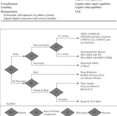
The petroleum and chemical industries have for many years been the traditional users of thermodynamic data, though the polymer, pharmaceutical and other industrial sectors are today making use of thermodynamic tools. Moreover, thermodynamic data are important for product design and certain applications in the environmental field, e.g. estimation of the distribution of chemicals in environmental ecosystems. Already several commercial simulators have a wide spectrum of thermodynamic models to choose from and companies often use the so-called ‘decision or selection trees’, see Figure 1.1, for selecting models suitable for specific applications, either those developed in-house2or those suggested by the simulator providers.3
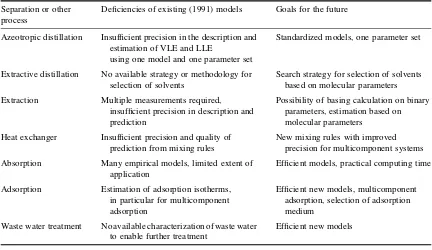
Still, it is often questioned whether sufficient data and/or suitable models are available for a particular process or need. Opinions differ even within the same industrial sector and they should also be seen in relation to the time that the various statements have been made.4,5The needs, even within the same industrial sector, are not always the same. Dohrn and Pfohl6explain why, in the chemical industry, the answer to the question about the availability of thermophysical data can be almost anything from ‘we have enough data’, or ‘we don’t have enough data’, to ‘we have too much data’. These statements can be respectively justified based on the availability of suitable models in process simulators, the existence of difficult separations or the many databases which may be at hand. Data for multicomponent mixtures especially can be scarce and costly even for well-defined mixtures of industrial importance such as water–hydrocarbon–alcohols or glycols. Moreover, Dohrn and Pfohl6illustrate, using examples, how similar models may yield different designs even for rather ‘simple’ mixtures, e.g. in the case of ethylbenzene/styrene with the SRK equation of state. In an earlier study, Zeck7presents thermodynamic difficulties and needs, as seen from the chemical industry’s point of view. These are summarized in Table 1.2.
As both Tables 1.1 and 1.2 illustrate, different types of phase equilibria data or calculations are needed depending on the problem, especially the separation type involved. The fundamental phase equilibria
Thermodynamic Models for Industrial Applications: From Classical and Advanced Mixing Rules to Association Theories
Table 1.1 Phase equilibria data needed in the design of specific unit operations
Unit operation phase equilibria type
Distillation Vapor–liquid equilibria (VLE)
Azeotropic distillation VLE, liquid–liquid equilibria (LLE)
Extractive distillation LLE
Evaporation, drying Gas–liquid equilibria
Absorption VLE
Reboiled absorption Gas–liquid equilibria
Stripping Gas–liquid equilibria
Extraction LLE
Supercritical fluid extraction Gas–liquid and solid–gas equilibria
Adsorption Vapor–solid equilibria
Liquid–solid equilibria
Crystallization Liquid–solid (vapor) equilibria
Leaching Liquid–solid equilibria
Bioseparations LLE
Extraction with aqueous two-phase systems Liquid–liquid extraction with reverse micelles
PL?
R?
P? E?
PL? R? E? P?
Polar
Non-electrolyte
Electrolyte Electrolyte NRTL or Pitzer
Peng–Robinson, Redlich–Kwong–Soave Lee–Kesler–Plocker Real
Pseudo & Real
Chao–Seader, Grayson–Streed or Braun K-10
Vacuum
Braun K-10 or Ideal
Polarity Real or Pseudo-components Electrolyte Pressure Symbols:
P?
P < 10 bar
P > 10 bar
NRTL, UNIQUAC, WILSON and their variations, UNIFAC LLE, UNIFAC and its extensions
Schwartentruber–Renon, PR or RKS with WS, PR or RKS with MHV2, PSRK
All Non-polar
Figure 1.1 Available thermodynamic models in commercial process simulators and an example of a selection tree for
equation, which is the usual starting point for all phase equilibria problems, is the equality of the fugacities of all components at all phases (a,b,g,. . .):
^
fai ¼^fib¼^fgi ¼. . . withi¼1;2;. . .;N ð1:1Þ
whereNis the number of components.
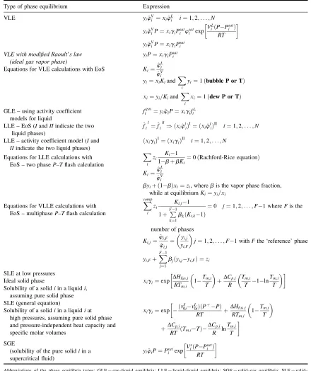
Equation (1.1) holds at equilibria for all compounds in a multicomponent mixture and for all phases (a,b, g, . . .). Using this equation, the ‘formal’ (mathematical) problem is solved. Fugacity coefficients can be calculated from volumetric data or alternatively from an equation of state (functions ofP–V–T). Physically, we can imagine that the fugacity is the ‘tendency’ of a molecule to leave from one phase to another. Phase equilibrium is a dynamic one, e.g. for VLE the number of liquid molecules going to the vapor phase is, at equilibrium, equal to the number of vapor molecules going to the liquid phase. The basic equation (1.1) may appear in different forms depending on the type of phase equilibria and even the nature of the thermodynamic model used (equation of state, activity coefficient). These forms are sometimes easier to use in practice than the general equation (1.1), although they are naturally all derived from this equation upon well-defined assumptions. The various forms of phase equilibria are summarized in Table 1.3, while Appendix 1.A presents some of the most important fundamental equations in thermodynamics which will find applications in the coming chapters. The principal thermodynamic models are the equations of state (EoS), which can be expressed as functions ofPðV;TÞorVðP;TÞ. The fugacity coefficient of a compound in a mixture can be calculated from any of the
Table 1.2 Thermodynamic challenges of interest to the process industry. After Zeck7 Separation or other
process
Deficiencies of existing (1991) models Goals for the future
Azeotropic distillation Insufficient precision in the description and estimation of VLE and LLE
using one model and one parameter set
Standardized models, one parameter set
Extractive distillation No available strategy or methodology for selection of solvents
Search strategy for selection of solvents based on molecular parameters
Extraction Multiple measurements required,
insufficient precision in description and prediction
Possibility of basing calculation on binary parameters, estimation based on molecular parameters
Heat exchanger Insufficient precision and quality of prediction from mixing rules
New mixing rules with improved precision for multicomponent systems
Absorption Many empirical models, limited extent of
application
Efficient models, practical computing time
Adsorption Estimation of adsorption isotherms,
in particular for multicomponent adsorption
Efficient new models, multicomponent adsorption, selection of adsorption medium
Waste water treatment No available characterization of waste water to enable further treatment
Table 1.3 Phase equilibrium equations in specific cases including basic equations for equilibrium calculations with equations of state (EoS). The fugacity coefficient of a compound in a mixture is defined asw^i¼^f=xiPi, where xican be the concentration in the liquid, vapor or solid phase. The vapor pressure Psatis obtained from correlations based, for example, on the Antoine equation or the DIPPR correlations
Type of phase equilibrium Expression
VLE yiw^Vi ¼xiw^Li i¼1;2;. . .;N VLE with modified Raoult’s law
(ideal gas vapor phase)
yiP¼xigiPsati
Equations for VLE calculations with EoS Ki¼^ wLi GLE – using activity coefficient
models for liquid LLE – activity coefficient model (Iand
IIindicate the two liquid phases)
ðxigiÞ I
¼ ðxigiÞ II
i¼1;2;. . .;N
Equations for LLE calculations with EoS – two phaseP–Tflash calculation
X
i zi
Ki 1 1 bþbKi¼
0ðRachford-Rice equationÞ
Ki¼
Equations for VLLE calculations with EoS – multiphaseP–Tflash calculation
X
Solubility of a solidiin a liquidi, assuming pure solid phase SLE (general equation)
Solubility of a solidiin a liquidiat high pressures, assuming pure solid phase and pressure-independent heat capacity and specific molar volumes
RTlnw^i¼RTln
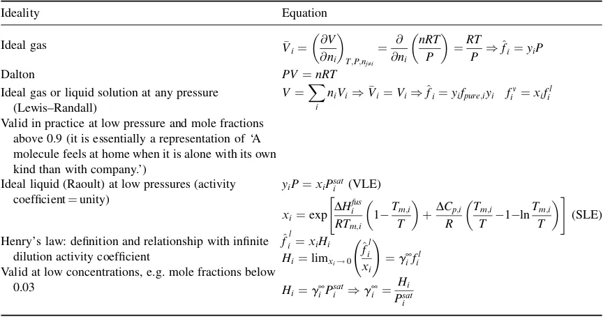
Equation (1.2) is most suitable for EoS of the typePðV;TÞ, while Equation (1.3) is suitable for EoS of the formVðP;TÞ. In principle, they are suitable for all types of fluid phases, conditions (T,P,concentration) and mixtures of any number of components. In practice, however, the situation can be quite different and equilibria types such as SLE, LLE and even complex VLE can often be conveniently handled with activity coefficient models, specifically developed for condensed phases (Table 1.3). Activity coefficients are useful means of representing deviations from ideality. In thermodynamics we picture as ideal the solutions which contain compounds with similar sizes and shapes and where the forces between like and unlike molecules are essentially the same, e.g. methanol/ethanol, pentane/hexane, benzene/toluene or mixtures of isomers. However, the phase equilibrium equations (for VLE and SLE) can take various forms depending on the precise conditions under which the solution is ideal. Ideal solutions do not separate into two liquid phases (i.e. no LLE is present). Table 1.4 summarizes the various definitions of ideality in thermodynamics.
We often use the terminologygamma–phi(g w) andphi–phi(w w) for the approaches, with the latter implying that an EoS is used for all phases, while in the former case an activity coefficient model is used for the liquid or solids phases. It is apparent from the above discussion that the distinction between thegamma–phi (g w) and phi–phi (w w) approaches is not of a fundamental character but rather a traditional (and somewhat old-fashioned) one. Such a distinction largely exists due to the fact that classical cubic equations of state EoS, which were the ‘first’ EoS in the market, in combination with the widely used van der Waals one-fluid mixing rules, are typically suitable ‘only’ for describing VLE of rather simple systems (e.g. mixtures of hydrocarbons and gases). Thus, numerous activity coefficient models have been developed since the early twentieth century, particularly for complex mixture VLE, LLE and SLE. Moreover, they provided a way for
Table 1.4 Ideality in thermodynamics. The Dalton, Raoult, Henry and Lewis–Randall ‘laws’
Ideality Equation
Ideal gas or liquid solution at any pressure (Lewis–Randall)
V¼X i
niVi)Vi¼Vi)^fi¼yifpure;iyi fiv¼xifil Valid in practice at low pressure and mole fractions
above 0.9 (it is essentially a representation of ‘A molecule feels at home when it is alone with its own kind than with company.’)
Ideal liquid (Raoult) at low pressures (activity coefficient¼unity)
Henry’s law: definition and relationship with infinite dilution activity coefficient
^
fil¼xiHi Valid at low concentrations, e.g. mole fractions below
fast, simple calculations in the mid twentieth century, when computers were not as powerful as they are today. In addition, activity coefficients help visualize the deviations from ideality, and, as Table 1.5 illustrates, activity coefficients can vary enormously, from far below unity, e.g. for polymer solutions, up to several million for ‘complex’ pollutants in water. This variation indicates the wide range of intermolecular forces, which are discussed in Chapter 2. In most cases, activity coefficient values are above unity (positive deviations from Raoult’s law). Negative deviations from Raoult’s law (activity coefficients below one) are present in mixtures exhibiting strong cross-interactions, e.g. chloroform–acetone and nearly athermal hydrocarbon and polymer solutions (mixtures with almost zero heat of mixing). Some common phase diagrams for binary mixtures are presented in Appendix 1.B.
The purpose of this book is not to discuss the ‘fundamentals of thermodynamics’, i.e. derivations and background of the equations shown in Table 1.3 or the numerical aspects of solving these equations. Excellent textbooks are available8–13with the last, by Michelsen and Mollerup, focusing especially on computational aspects of thermodynamic models. It is rather the purpose of this textbook to address how thermodynamics assisted by disciplines like physical chemistry and statistical thermodynamics ‘attempt’ to identify the ‘best’ model (EoS, activity coefficient) for specific applications, taking into account the peculiarities of the applications considered:
. For which phases can the model be applied (VLE, LLE, VLLE, SLE, SGE, etc.)? Is there a possibility for the existence of more than two phases at the same or different conditions (e.g. VLE at high temperatures and LLE at low temperatures)?
. Conditions (T,P, concentration).
. Peculiarities (e.g. azeotropic behavior, negative deviations from Raoult’s law). . Type of compounds (hydrocarbons, alcohols, water, polymers, electrolytes, etc.). . Number and nature of interaction parameters – how can they be obtained?
Table 1.5 Typical values of infinite dilution activity coefficients in aqueous systems. Activity coefficient values can be sometimes useful in determining whether phase splitting will occur, as miscible systems have in most cases activity coefficients below 10, while very immiscible systems have activity coefficients above 200, and the activity coefficients of partially miscible systems typically lie in between these two values
Compound Activity coefficient of water at
infinite dilution in the compound
Methyl ethyl ketone 32
Diethyl ether 160
Chloroform 860
Carbon tetrachloride 10 000
Ethyl acetate 150
Octanol 3700
Benzene 2400
Toluene 12 000
Naphthalene 140 000
Phenanthrene 7 400 000
Hexachlorobenzene 980 000 000
Adenine 7200
. Are the models suitable for correlation (description) and/or prediction of phase behavior (i.e. calculations when no experimental data are available for determining the model parameters)?
. Simplicity vs. complexity – speed of calculations.
. Performance for multicomponent systems (parameters obtained from binary data).
While specific thermodynamic models often ‘come and go’, certain general theories, concepts and principles do stay or apply in many models. Examples of such theories and concepts are: group contribution, local composition, corresponding states principle, solubility parameters, free volumes, mixing and combining rules, and association theories (chemical-like, lattice and perturbation theories). It is also the purpose of this book to highlight these concepts and their use in thermodynamic models.
Clearly, a thorough understanding of intermolecular forces is useful both in the interpretation of phase behavior and in the choice and in some cases development of improved models. A short ‘practical’ introduction on the intermolecular and interparticle forces is presented in the next chapter.
In conclusion, chemical engineering thermodynamics and in particular phase equilibria are important in both process and product design. Different types of phase equilibria (VLE, LLE, SLE, etc.) are important, depending on the application, especially the type of separation method used. The starting point for representing phase equilibria with thermodynamic models is the concept of equality of fugacities in all phases, a criterion which can take more readily used forms depending on the equilibrium type, as shown in Table 1.3. VLE is often easier to represent with thermodynamic models than LLE and VLLE provided that the ‘end-points’ of a VLE phase diagram (vapor pressures) are well reproduced. Azeotropic mixtures may be more difficult to represent than non-azeotropic ones. LLE phase diagrams for non-polymeric mixtures are typically of the upper critical solution temperature (UCST) type and often rather symmetric with respect to concentration, while LLE for polymer solutions is concentration asymmetric and often both UCST and LCST (Lower Critical Solution Temperature) types of behaviors are present. An auxiliary property typically used for representing phase equilibria of complex mixtures is the activity coefficient, which represents deviations from the ideal behavior as expressed by Raoult’s law. Experimental activity coefficient data can be obtained from VLE or SLE data. There are no general thermodynamic models which can describe equally successfully all types of phase equilibria at all conditions. Suitable models for high- and low-pressure phase equilibria for simple as well as complex mixtures including those with solids, polymers, electrolytes and associating fluids will be presented in this book.
1.1
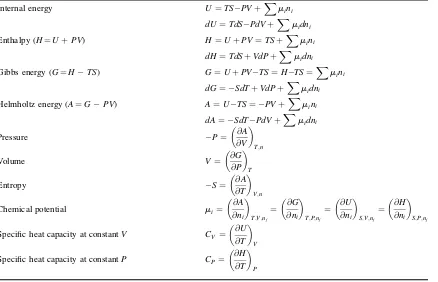
Appendix 1.A
Important equations from the framework
of thermodynamics
1.A.1 Excess and mixing properties
For any propertyM, e.g.V,H,S, etc., the excess (E) and mixing (mix) values are defined as:
DMmix¼M PixiMi
ME ¼DM
mix DMidealmix
ð1:4Þ
This means that forVandH, whereDVideal
mix ¼0;DHidealmix ¼0, we have:
DVmix¼VE
DHmix¼HE
This is not the case for the Gibbs energy or Helmholtz energy, because of the entropy term:
1.A.2 Excess Gibbs energy, fugacities and activity coefficients
These are as follows:
Table 1.6 Thermodynamic functions and partial derivatives
Internal energy U¼TS PVþXmini
Specific heat capacity at constantV CV ¼
@U
@T
V
Specific heat capacity at constantP CP¼
@H
@T
1.A.3 Deriving activity coefficients (gi) and activities (ai) from the excess Gibbs energy and the Gibbs energy change of mixing
The equations are:
RTlngi¼
@GE
@ni
T;P;nj„i
¼ @ng
E
@ni
T;P;nj„i
ð1:12Þ
lnai¼
@ @ni
nDGmix
RT
T;P;nj„i
ð1:13Þ
1.2
Appendix 1.B
Common phase diagrams for binary mixtures
and phase envelopes
Figure 1.2 (left) presents aPxydiagram for the binary mixturen-propanol–water at 363.15 K. The lower curve is the dew point curve; below this curve and for any concentration ofn-propanol the mixture is vapor. The upper curve is the bubble point curve and for any pressure higher than the bubble point curve the mixture is liquid. At a given composition the pressure along the bubble point curve is the pressure where an infinitesimal bubble of vapor coexists with the liquid, while for pressures between the dew point and bubble point curve the two different phases (vapor and liquid) coexist. Similar observations can be made for theTxydiagram presented in Figure 1.2 (right).
The shape of thePxyorTxydiagram indicates the deviation from the ideal solution behavior. For mixtures that exhibit moderate deviations from ideal solution behavior such as methanol–ethanol (see Figure 1.7 of Problem 2 on the companion website at www.wiley.com/go/Kontogeorgis) no azeotrope is formed. In the case of larger deviations, and in particular when the mixture components have comparable pure component vapor
pressures, an azeotrope may form. A typical example is shown in Figure 1.2 for mixtures that exhibit positive deviations from Raoult’s law; this azeotrope is called minimum boiling since the azeotropic composition at a given pressure has the lowest boiling temperature, as shown in Figure 1.2 (right). Negative deviations from Raoult’s law are rather rare; they are found in cases where the components form hydrogen bonds with each other, e.g. when one compound is an electron acceptor and the other an electron donor. Chloroform–acetone is a classical example of a maximum boiling azeotrope, as presented in Figure 1.3.
A more complex phase diagram is presented in Figure 1.4, for the mixture methanol–n-heptane at atmospheric pressure. The VLE of the mixture is similar to the one presented in Figure 1.2 exhibiting positive deviations from Raoult’s law. As already mentioned, below the bubble point curve a single liquid phase is formed. However, when the temperature is further decreased, and depending on the relative concentration of methanol andn-heptane, the mixture becomes partly immiscible and an additional liquid phase is formed. The left part of the LLE curve corresponds to the solubility of methanol in the hydrocarbon phase (i.e.n-heptane-rich phase), while the right part represents the solubility of methanol in the polar phase (i.e. methanol-rich phase). The LLE curve is called binodal and ends at the upper critical solution temperature, which is the highest temperature where the mixture is still partly immiscible.
Figure 1.5 presents the phase envelope (PTdiagram) of the binary mixture ethane–heptane (C2–n-C7)
with the SRK EoS. As can be seen, a typical phase envelope consists of two lines, the dew point line and the bubble point line. The phase envelope separates the single phase region from the two-phase region. At pressures above the bubble point the fluid is in liquid form. At pressures below the bubble point curve, the mixtures separate into two phases, a vapor phase and a liquid phase. The remaining part of the curve is the dew point line. The effect of varying concentration on the phase envelope is also apparent, since different concentrations result in different curves and different critical points. The critical line (or critical locus) of the binary system is also presented on the phase diagram. The critical line represents thePTcurve through all possible critical points for mixtures of the two components, from pure ethane to pure heptane. The dew point line and the bubble point line are the same curve for a pure component, called the vapor pressure curve.
Figure 1.6 presents a classical phase envelope for a seven-component natural gas mixture. At the critical point the liquid and the vapor have identical properties. The point of maximum pressure on the phase diagram (140.3 bar) is called cricondenbar and the point of extreme temperature cricondentherm (336 K). The phase diagram of Figure 1.6 shows an interesting phenomenon, called retrograde condensation. Normally, an
0 10 20 30 40 50 60 70 80 90 100
550 450
350 250
150
T / K
P / bar
Dew point line Bubble point line Critical point pure heptane pure ethane critical line
Figure 1.5 Phase envelopes for the ethane–heptane binary mixture with the SRK EoS and kij¼0 at different
concentrations. The vapor pressure curves of pure ethane (solid curve) and heptane (dashed curve) are also presented: for a pure component, the bubble point and the dew point lines merge in the vapor pressure curve
increase in pressure leads to increased condensation (formation of liquid) and a reduction to reduced liquid formation. Consider now the natural gas mixture in the figure at a temperature of 320 K. As can be seen in Figure 1.6, at a pressure of 130 bar we are in the single phase (vapor) region; a decrease in pressure leads to the formation of a liquid phase, while upon further reduction of the pressure we observe the usual behavior, i.e. the condensed liquid re-evaporates, and below the dew point curve a single vapor phase is again obtained. Retrograde phenomena are common in gas reservoirs and a proper understanding of retrograde behavior is important for efficient production.
This discussion is limited to common phase envelopes. Unusual phase envelopes, however, also exist. Atypical phase envelopes can have two critical points: phase envelopes with an almost vertical increase in pressure at a given temperature (as a result of an LLE) at the phase boundary, or phase envelopes with no critical point location (as a result of a phase split in three phases in the area where the critical point would have been located in case the mixture were a two-phase one). Michelsen and Mollerup13discuss such unusual phenomena in more detail.
References
1. J.M. Prausnitz, R.N. Lichtenthaler, E.G. de Azevedo,Molecular Thermodynamics of Fluid-Phase Equilibria( 3rd edition). Prentice Hall International, 1999.
2. G.M. Kontogeorgis, R. Gani, Introduction to computer aided product design. In: G.M. Kontogeorgis, R. Gani,
Computer-Aided Property Estimation for Process and Product Design. Elsevier, 2004. 3. E.A. Carlson,Chem. Eng. Prog.,1996, October, 35–46.
4. C. Tsonopoulos, J.L. Heidman,Fluid Phase Equilibr.,1986,29, 391–414. 5. S. Gupta, J.D. Olson,Ind. Eng. Chem. Res.,2003,42(25), 6359–6374. 6. R. Dohrn, O. Pfohl,Fluid Phase Equilib.,2002,194–197, 15–29. 7. S. Zeck,Fluid Phase Equilib.,1991,70, 125–140.
8. J.M. Smith, H.C. van Ness, M.M. Abbott,Introduction to Chemical Engineering Thermodynamics(7th edition). McGraw-Hill International, 2005.
0 20 40 60 80 100 120 140 160
350 300
250 200
150 100
T / K
P / bar
Dew point line Bubble point line Critical point Cricondenbar Cricondentherm