Advanced Excel Essentials Ebook free dowwnload

(1)

•฀฀How฀to฀write฀optimized฀code฀and฀formulas฀that฀are฀easily฀understood฀

•฀฀How฀to฀turn฀a฀spreadsheet฀into฀a฀powerhouse฀application฀that฀rivals฀

(2)

For your convenience Apress has placed some of the front

matter material after the index. Please use the Bookmarks

(3)

Contents at a Glance

Chapter 1: Introduction to Advanced Excel Essentials

■

...3

Chapter 2: Visual Basic for Applications for Excel, a Refresher

■

...11

Chapter 7: Storage Patterns for User Input

(4)

PART I

Core Advanced Excel Concepts

In this part, I’ll review the core concepts that make up the essentials of advanced Excel.

Chapter 1 explains what is meant by advanced Excel development, and how this book differs from many others. For instance, several books place significant emphasis on Visual Basic for Applications code, believing macros to be the most important feature of Excel development. This chapter will challenge that notion and present advanced concepts as a product of many different Excel features, including code. Additionally, I discuss the most important required skill—creativity.

Chapter 2 provides a brief Visual Basic for Applications refresher. I’ll discuss how best to set up the coding environment to make it conducive to headache-free coding. I’ll also challenge conventional coding conventions and propose alternatives that will prove more effective.

Chapter 3 introduces the formula concepts that will be used in this book. The chapter starts with tips that will make your experience developing advanced formulas run more smoothly. I’ll then show you how to perform advanced calculations by simply using range operators. You’ll develop advanced alternatives to the IF function that will prove more powerful in practice and more readable later on. In addition, you’ll

investigate the full extent of Excel’s Boolean logic features.

Chapter 4 continues the discussion of formulas by demonstrating how they can be used with advanced applications. I take you through several examples applying these formula concepts and demonstrate how they can be understood with a little bit of algebra. The chapter concludes by introducing the notion of reusable components, which are spreadsheet mechanics that can be easily reused for other projects.

(5)

Introduction to Advanced Excel

Essentials

I set out to write a book on the essentials of Excel development—that is, a book that concisely presents many of the development principles and practices I’ve discovered through my work and consulting experience.

But whether on purpose or by accident, this book has become something considerably more than that. Indeed, another name for this book could be A Contrarian’s Guide To Excel Development. You see, this book will push back against the wisdom of other terrific Excel books, including my favorite book, Professional Excel Development

(Addison-Wesley 2005). To be sure, the information in those books is terrific, and whatever merits this book might achieve, it will likely never come close to the impact of Professional Excel Development.

At the same time, much of the information in these books, I believe, is somewhat dated. For instance, let’s take the case of Hungarian Notation. Hungarian Notation is a variable naming convention encouraged by virtually all Excel development books. Even if you’ve never heard of Hungarian Notation, you’ve likely seen and used it, if you’ve ever looked at or learned from example code. It basically says a variable’s name should start with a prefix of the variable’s type. For instance, lblCaption, intCounter, and strTitle are all examples of Hungarian Notation: the lbl in lblCaption tells us we’re working with a Label object; the int in intCounter tells us we’re working with an integer type, and the str in strTitle tell us we’re working with a string type. If you’ve done any VBA coding before, this is likely not new information.

You might not know this, however: most modern languages have all but abandoned Hungarian Notation. Microsoft’s .NET style guidelines, for instance, even discourage its use. More than a decade has passed since Microsoft last recommended Hungarian Notation. I argue that it’s time for a more modern naming style, which I introduce in Chapter 2.

But this book is concerned with more than just naming conventions. I argue that we should change the way we think about development. Previous books have placed significant emphasis on user interface with ActiveX objects and UserForms. This book will eschew these bloated controls; rather, this book will show you how to develop complex interactivity using the spreadsheet as your canvas. You’ll see that it’s easier and provides for more control and flexibility compared to conventional methods from other books.

In addition, I’ll place less emphasis on code and a stronger emphasis on formulas (Chapters 3, 4, and 5). Many books have narrowly defined the principles of advanced Excel in terms of VBA code. But formulas can be powerful. And often they can be used in place of VBA code. You might be surprised by how much interactivity you can create without writing a single line of code. And how much quicker your spreadsheet runs because of it.

(6)

CHAPTER 1 ■ INTRODUCTION TO ADVANCED EXCEL ESSENTIALS

However, if you learn anything from my book, it should be that the process of development never stops.

The most important skill you’ll need is creativity. Just as I saw different ways to approach a problem than my predecessors, so too should you analyze what’s being presented to you. Undoubtedly, you’ll find even better approaches than I did. I don’t expect everyone to agree with my approaches, but what’s important is that you understand them, so you can see what works, what doesn’t, and why. Because you won’t become an advanced Excel developer through rote memorization of the material presented herein; you must learn to think like an advanced developer. This book will teach you the essentials of doing just that.

What to Expect from this Book

This is not a beginner level book. I assume you have intermediate level experience with formulas and Visual Basic for Applications. At the very least, you should be able to understand and write both formulas and code. Complete mastery isn’t necessary; because the topics presented in this book are somewhat new, a mastery in these topics might not even help you. All that being said, if you’re an experienced Excel user—and you have the aptitude and thirst to learn new things—there’s no reason you won’t be successful in reading this book! Again, the most important (and cherished) skill that will guarantee your success is creativity.

What’s considered “advanced” may mean different things to different people. Here, we’re interested in the principles that help us become better spreadsheet users and developers. That said, this book will make use of Excel features such as formulas, tables, conditional formatting, Visual Basic for Applications code, form controls, and charts. For the most part, I will present a brief refresher on what these features do and how they are used. However, you’ll find this book moves at a quicker pace than beginner level treatments for these items. Features such as PivotTables, PowerPivot, Power Map, and data tables are not discussed in this book. But you’ll find that the principles presented in these pages are extendable to these topics.

Indeed, this book is most concerned with teaching Excel development as first principles. I will explain what they are and how best they are used in practice. Once you learn underlying concepts, extending their use into applications becomes trivial.

Example Files Used in This Book

This book comes with many examples as a complement to the material presented herein. The example files are organized by chapter. Whenever there is a corresponding example file for the material presented, I’ll provide you the name of the example file in the text. All example files are freely available to download from the book’s Apress web page (www.apress.com/9781484207352). The files are designed to work in Excel 2007 and newer.

The Two Most Important Principles

There are many different ideas and concepts presented in this book. But I’ll be daring and attempt to sum them up as two key concepts:

1. When it make sense, do more with less.

2. Break every rule.

Note

(7)

When It Makes Sense, Do More with Less

You don’t need VBA to do everything. Many times, the reason a spreadsheet is slow is because there is too much reliance on code. Similarly, too many formulas—especially volatile functions like OFFSET and INDIRECT—will almost always slow down a spreadsheet. There are better alternatives to these methods. Often, they require less code and can get more done.

However, we should be wary of brevity for the sake of it. Bill “MrExcel” Jelen and I have a friendly disagreement1 on whether to use Option Explicit in your code. He says he doesn’t need it because he always writes perfect code to start with—and that its use needlessly adds more lines of code. I, of course, respectfully disagree. I strongly encourage you to use Option Explicit. Option Explicit requires that you declare your variables before they’re used. That means that you cannot introduce a new variable in your code on the fly. Listing 1-1 shows code without Option Explicit; Listing 1-2 shows code with Option Explicit.

Listing 1-1. No Option Explicit

Public Sub MyResponse()

ResponseMessage = "Code Executed Successfully!" MsgBox ResponseMessage

End Sub

Listing 1-2. With Option Explicit

Option Explicit

Public Sub MyResponse()

Dim ResponseMessage as String

ResponseMessage = "Code Executed Successfully!" MsgBox ResponseMessage

End Sub

Bill argued using Option Explicit required at least one additional line of code for every variable. And it might appear Listing 1-1 is indeed doing more (or at least the same) with less code. But, as I show in Chapter 2, not using Option Explicit might be more trouble than it is worth. Debugging is much harder without Option Explicit, and not using it even encourages sloppy code. From my standpoint, leaving out Option Explicit (and the required variable declaration) is simply getting less done with less code. But however you feel on this particular issue, it’s worth testing your opinion against that first principle: ask yourself, am I really doing more with less?

Break Every Rule

I truly believe, and stand by, the material presented in this book. But I would have never discovered any of it without departing from conventional wisdom. Again, I’ll keep hammering this point until I am blue in the face: the most important takeway from this book is creativity. And you cannot be creative without pushing a few boundaries. Don’t be scared to crash a spreadsheet or two in the pursuit of learning.

(8)

Most important, you shouldn’t be satisfied with Excel’s perceived limitations. Over the last several years, I’ve been blown away by what I’ve seen others accomplish with Excel. There is a thriving online community dedicated to helping people realize their imaginations with spreadsheets. Whenever I need inspiration, I look to the community.

For your own consideration, I’ll provide two examples of my own work that show what can be done with Excel when we think creatively. Figure 1-1 shows a three dimensional maze I created. It might surprise you to learn there is very little code involved. And the “maze” is simply an area chart formatted to look like a three dimensional plane.

Figure 1-1. A three dimensional maze, made with Excel

(9)

Both the three dimensional maze and periodic table are available for you to investigate in the project files included with this book. While it’s beyond the scope of this book to explain in detail how these particular spreadsheets were created, they are the direct product of the material I present in the rest of the book. However, if you’re interested in reading how these items were developed, see the links in the sidebar.

LINKS ON DEVELOPING A MAZE AND MOUSE OVER MECHANISM

How to Create a Rollover Effect in Excel: Execute a Macro When Your Mouse is Over a Cell

http://optionexplicitvba.blogspot.com/2011/04/rollover-b8-ov1.html

Roll Over Tooltips and Web Actions on a Microsoft Excel Dashboard

www.clearlyandsimply.com/clearly_and_simply/2012/11/roll-over-tooltips-and-web-actions-on-a-microsoft-excel-dashboard.html

Development Principles for Excel Games and Applications

http://optionexplicitvba.com/2013/09/16/development-principles-for-excel-games-and-applications/

Your First Maze

(10)

Available Resources

As I said in the previous section, sometimes you need some inspiration to help get you going. Here’s a list of resources I use regularly.

Google

Google...Google...Google! Google is your best friend. If you’re ever stuck on a problem, simply ask Google the same way you might your friend. Usually, you’ll find the results in Excel forums where folks have asked the very same questions.

Chandoo

This site, by Purna “Chandoo” Duggirala, is a phenomenal resource for every Excel developer, from novice to professional. Chandoo covers many topics including dashboards, VBA, data visualization, and formula techniques. His site is also host to a thriving online forum community.

www.chandoo.org

Cleary and Simply

Clearly and Simply is a site by Robert Mundigl. The site is mainly focused on dashboards and data visualization techniques with Excel and Tableau.

www.ClearlyAndSimply.com

Contextures

Debra Dalgleish runs the Contextures web site, which focuses on Excel development and dashboards, particularly with PivotTables. Her approach to dashboards and the use of PivotTables is different from mine, but well worth a read. She is also the author of these Apress Books:

•฀ Excel Pivot Tables Recipe Book: A Problem-Solution Approach

•฀ Beginning PivotTables in Excel 2007: From Novice to Professional

www.contextures.com

Excel Hero

Excel Hero was created by Daniel Ferry. While his blog is not very active anymore, you will find his older content incredibly useful. Several of his articles have served as the inspiration for the content found in these pages.

www.ExcelHero.com

Peltier Tech

Jon Peltier is a chartmaster. His web site is full of charting tutorials and examples. He provides sage wisdom on data

visualization and proper data analysis. His web site covers every conceivable thing you might want to do with a chart in Excel.

(11)

The Last Word

(12)

CHAPTER 2 Visual Basic for Applications for

Excel, a Refresher

Of course, no advanced book on developing anything in Excel would be complete without a chapter on the interpreter language housed within Excel, Visual Basic for Applications–or better known by its shorthand moniker, VBA.

This chapter won’t be an introduction to VBA but rather a review of VBA programming techniques and development principles found in this book and practiced throughout most of my career. What follows may appear unconventional, at first. Indeed, it may differ somewhat from what you’ve been previously taught. However, I don’t leave you with a few instructions and no guidance. Instead, I’ll explain in detail why I believe what I believe—and why you should believe as I do. If you find that you don’t—and I certainly welcome disagreement—consider the other important—actually, more important—takeaway from this chapter: the code choices and styles we use should always follow from a set of principles, guidelines, and convention. When you code, do so with structure and meaning. Know

why you believe what you believe.

But, the most important thing to do right now is to ready yourself to begin coding. This requires that you set the right conditions in your coding environment.

Making the Most of Your Coding Experience

(13)

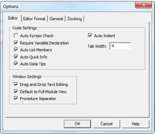
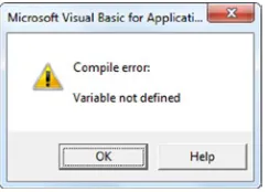
Tell Excel: Stop Annoying Me!

I mean, nobody’s perfect, but you don’t need this popup ruining your coding flow every time you click to another line. So, save yourself from unnecessary popups by disabling Auto Syntax Check from the Options dialog box, which you access by selecting Tools > Options (see Figure 2-2). This will only disable the popup. The offending syntax error is still highlighted in red—in other words, you don’t lose any functionality, just the annoyance.

(14)

CHAPTER 2 ■ VISUAL BASIC FOR APPLICATIONS FOR EXCEL, A REFRESHER

Make Loud Comments

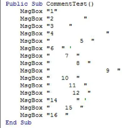
If you comment your code regularly—and you should—you’ve probably noticed comments don’t “stand out” very much. In fact, I’ll be the first to admit I’ve gone through code and missed comments because they’ve “blended in” with their surroundings. Figure 2-3 shows perhaps a more extreme example involving rather busy code, but the point remains: the two comment markers (') I’ve placed in the routine are not easily or immediately found.

Figure 2-3. Comment markers at 6 and 14 blend in with the code

(15)

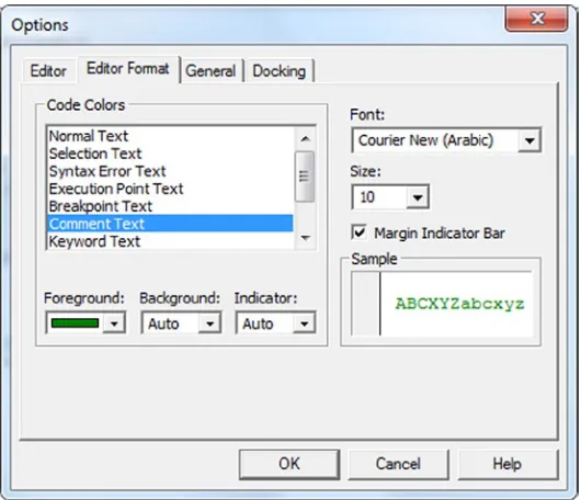
Figure 2-5. Let your comments be heard with bold colors

Figure 2-4. The Editor Format dialog box

Pick a Readable Font

(16)

You can change the font by selecting Normal Text from the list box (Figure 2-4) and using the font dropdown on the side of the dialog box. Excel gives you lots of fonts to choose from, but the best fonts with which to code are those of fixed width. So if you choose something other than Consolas or Courier New, make sure to pick a readable, fixed-width font.

Start Using the Immediate Window, Immediately

The Immediate window is like a handy scratchpad with many uses. If the Immediate window is not already open, go to View ➤ Immediate Window in the Visual Basic Editor. You can type calculations and expressions directly into the Immediate window using the print keyword. Figure 2-8 provides some examples of typing directly into the Immediate window.

Figure 2-6. Sample code with Courier New as the font

Figure 2-7. More readable text with Consolas

(17)

In addition, you can also print the response of a loop or method directly into the Immediate window. To do this, use Debug.Print. Listing 2-1 shows you how.

Listing 2-1. Using Debug.Print to Write to the Immediate Window While in Runtime

For i = 1 to 100

Debug.Print "Current Iteration: " & i Next i

Debug.Print "Loop finished."

Opt for Option Explicit

VBA doesn’t require you declare your variables before using them—that is, unless you place the words Option Explicit at the top of your code module. Without Option Explicit, the For loop from Listing 2-1 would run without problems. When you use Option Explicit, you must declare all variables before they are used. In Listing 2-2, I’ve used the Dim keyword to declare the integer i.

Listing 2-2. A For-Next Loop with Declared Variables

Dim i as Integer For i = 1 to 100

Debug.Print "Current Iteration: " & i Next i

Debug.Print "Loop finished."

If you forgo Option Explicit, as I did in the first instance, Excel will simply create the variable i for you. However, that i won’t be an integer; rather it will be of a variant type. This may not sound like such a bad thing at first, but letting Excel simply make variables for you is a recipe for trouble. What if you misspell a variable, like RecordCount, as I’ve done in Listing 2-3?

Listing 2-3. An Example of a Variable Created on the Spot Because Option Explicit Wasn’t Used

RecordCount = 1 Msgbox RecordCout

Excel won’t alert you to an error. Instead, it will simply create RecordCout as a new variable. Do you trust your ability to find misspellings in your code quickly?

(18)

Seriously, I can’t tell you how important Option Explicit is. I’d repeat “Always use Option Explicit!” 1,000 times here if I could. But I’ll just let Excel do it for me instead. Paste the following formula into an empty cell before moving to the next section.

=REPT("Always use Option Explicit! ",1000)

Naming Conventions

A naming convention is a common identification system for variables, constants, and objects. By definition, then, a good naming convention should be sufficiently descriptive about the content and nature of the thing named. In the next subsections, I’ll talk about two naming conventions. The first, Hungarian Notation, is the most common notation used for VBA coding. Indeed, I’m unaware of any book that has argued against its use—that is, until now. The second, my preferred notation, is what I call “loose” CamelCase notation, and it’s similar to the standard for just about all modern object-oriented languages.

Hungarian Notation

In this section, I’ll talk about Hungarian Notation. In this notation, the variable name consists of a prefix—usually an abbreviated description the variable’s type—followed by one or two words describing the variable’s function (e.g. its reason for existing). For example, in Listing 2-4, the “s” before Title is used to indicate the variable is of String type. The term “title,” as I’m sure you can guess, describes to the string’s function—in other words, its reason for existing.

Listing 2-4. An Example of Hungarian Notation

Dim sTitle as String

sTitle = “The new spreadsheet.!”

Table 2-1 shows some suggested prefixes for common variables and classes.

Table 2-1. Prefixes Suggested by Hungarian Notation

(19)

In this book, I will discourage the use of Hungarian Notation in your code. I’m not here to tell you that Hungarian Notation is terrible because it does have its uses. For instance, VBA code isn’t known for having very strict data type rules. This means you can assign integers to strings without casting from one type to the other. So including the type in a variables name isn’t a terrible idea at all.

But much of this type confusion can be resolved by using descriptive and proper variables names, as you’ll see in the next few pages. For now, however, it’s a good idea to at least familiarize yourself with Hungarian Notation if you haven’t done so already. Hungarian Notation is still widely used in VBA to this day, so it’s important that you can read it proficiently even if you decide in this moment to never use it again. (Good choice!)

The fact is, Hungarian Notation is old. Indeed, in many ways, it’s a relic of a bygone era–namely, the era in which people still used Visual Basic 6.0. (Those were the days, right?) In fact, Microsoft’s Design Guidelines for .NET libraries has discouraged its use for more than decade. So what I’m proposing in this next section might feel new, but it’s actually been around for quite some time.

“Loose” CamelCase Notation

In this section, I’ll talk about loose CamelCase notation as my preferred alternative. CamelCase notation begins with a description (with the first letter in the “lower case,” when it’s a local, private variable—hence the name “CamelCase”) and usually ends with the object type unabbreviated. For example, the variable in Listing 2-5 refers to chart on a worksheet for sales.

Listing 2-5. A Demonstration of Camel Back Notation

Dim salesChart as Excel.Chart

Set salesChart = Sheet1.ChartObjects(1).Chart

I’ll be honest and admit I’m not always such a stickler about that lower case descriptor, which is why I call my use of this notation “loose.” The important takeaway when using this notation is to use very descriptive names. It’s unlikely a variable name like ChartTitle will be confused for an integer in your code. Whether it’s recordCount or RecordCount, you’ll likely understand that count refers to a nonnegative integer.

My rule of thumb is, local primitive types should start with a lower case, if you feel so inclined. Variables that represent objects should end with the object name unabbreviated. Notice in Listing 2-5 that the variable name ends with Chart. Ranges should end with Range, etc.

Descriptive names are important. Use a variable name that describes what the variable does so when you come back to it later, you can remember what you did. If you have a test variable, then (please, for the love of God) call it “test,”; don’t just call it “t.” It’s OK to use i in a For/Next loop where the i is simply an iterator and is not used later in the code, but don’t name variables used to count objects with short names like i,j,k,a,b,c. Finally, there’s really no good reason to use an underscore in your variable names. They’re not easier to read.

Named Ranges

As I said above, naming convention goes beyond just VBA. Indeed, a proper naming convention should be applied to all Excel objects, including those that reside on a spreadsheet. Therefore, in this section, I’ll talk about naming objects on the spreadsheet in the form of named ranges.

(20)

In Figure 2-10, the name of the tab is combined with the variable. Aside from being more object-oriented-ish, this type of naming brings other distinct advantages. For one, you can more easily and logically group named ranges that exist on the same worksheet tab. In addition, as you’ll see in the next section, this type of convention works very well when interfacing between named ranges and VBA.

Sheet Objects

In this section, I’ll focus on naming conventions for sheet objects. There’s one property of the sheet object that I’m a big fan of changing, and it’s the name of the object itself. When you change the name of a worksheet tab on the spreadsheet, you’re actually changing the name of the tab (think of it as changing a caption); you are not, in fact, changing the name of the worksheet object itself.

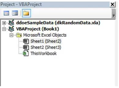
If for nothing else, changing the name of the worksheet object is a great way to clear up confusion when looking at the Project Explorer window. For example, Excel seems to have a problem keeping the names of worksheet tabs and the names of the objects themselves straight, as I’m sure you’ve noticed before. Take a look at Figure 2-11 to see what I mean.

Figure 2-10. An object-oriented like naming convetion for named ranges

(21)

The object name is the item outside the parenthesis; the tab name is the one inside the parenthesis. If I were to write MsgBox Sheet1.Name in the Immediate window, I would see a response of “Sheet2.”

To change the name of the object itself, go to the Properties window from within the editor (View ➤ Properties Window, if it’s not already visible) and change the line that says (name). In Figure 2-12, my worksheet tab’s caption is “Financial Data,” so I’m going to change its object name to FinancialData.

Figure 2-12. The Properties Explorer showing how to change the worksheet object’s name

YES, I KNOW IT’S CONFUSING

If you look at the Project Explorer window (Figure

2-12

, above), you’ll see that the worksheet object name comes

first and the tab name follows in parenthesis. The Properties Explorer window appears to do just the opposite;

the first name in parenthesis, “(name)”, refers to the object’s name, while the second name item (under Enable

Selection) refers to its name as it appears on the tab. Why did Microsoft choose to do it this way? Your guess is as

good as mine.

Referencing

In this section, I’ll talk about referencing. Referencing refers to interacting with other worksheet elements from within VBA code and also on the worksheet. This is where a good naming convention and proper coding style really makes the difference.

(22)

Shorthand References

This section discusses shorthand references, a syntax you can use in your code to refer named range on a sheet. Here is where the advantage of the latter notation proves its worth. As you know, you can refer to a named range through the sheet object where the name resides (technically, you can refer to it through any sheet object, but only on the worksheet in which it was created will it return the correct information). So, the typical way to read from or assign to the Cost of Goods Sold named range above using Hungarian Notation might look like this this:

Worksheets("Income Statement").Range("valCoGS").Value

On the other hand, if you use my method, you can employ the shorthand range syntax as follows:

[IncomeStatement.CostOfGoodsSold].Value

That’s right! These two lines of code mean and do the exact same thing. Now, which do you think is easier to read and is more descriptive of what it represents? Which more easily captures the worksheet in which it resides? Which would you rather use in your code?

Ok, so before you go off using the shorthand notation for everything, I should point out a significant caveat. Using the shorthand brackets method can become, in certain situations, slow. Technically, it’s a slower operation for Excel to complete than using a Worksheet object. However, you would really only notice this if you use the shorthand notation during a very long and computationally expensive loop. For typical code looping, you’re not likely to see the difference, but if you’re looking to speed things up inside a loop, it’s best to forgo the shorthand.

Worksheet Object Names

In the previous section, I showed you how to change the worksheet object names. In this section, you’ll see why I think it’s such a good idea.

Think about what you can do with this change. Because the new name reflects some descriptive information about the worksheet tab, you can use the object itself instead of the Worksheets() function to return the one you’re interested in. Confused? Let’s take a look. Here’s the old way, which takes in the Worksheet’s tab name to return the worksheet object:

Worksheets("Income Statement").Range("A1")

And here’s what you can do instead:

IncomeStatement.Range("A1")

Again, which do you think easier to understand and work with?

Procedures and Macros

In this section, I’ll talk about the benefit of changing sheet names on procedures. Once you’ve changed the procedure name, you can also place your macro into the sheet object itself.

(23)

Development Styles and Principles

Now that you’ve set up your coding environment and I’ve talked about naming conventions, I need to talk development styles and principles. The following is a list of simple coding guidelines that if you stick to, you’ll be creating self-contained, easy-to-follow code and design in no time. The first principle follows naturally from the last section.

Strive to Store Your Commonly Used Procedures in

Relevant Worksheet Tabs

If you’re an avid user of the Macro Recorder you know that Excel writes what you do to an open module. In many ways, a module feels like a natural place for a procedure. But ask yourself, is there any real reason why you’re storing the procedure there?

(24)

If you create this direction mechanism via the module method, you get ugly navigational code like in Listing 2-6. I also assume in Listing 2-6 that you’re doing some type of processing work where the user goes from a different worksheet tab back to Main.

'Link back to Main from each screen Public Sub From_Config_Goto_Main()

(25)

What do I mean by ugly? Well, creating this mechanism in a module requires you use funky procedure names to differentiate one from the other. And just take a look at what each of these procedures look like in the Macro dialog box (Figure 2-15). Each of these names looks so similar. It would be very easy to accidentally assign the wrong macro. (Are you nodding your head because you’ve done it before!? I know your pain.) In addition, even if you store procedures in separate modules, there’s nothing in the Macro dialog box to differentiate for this type of organization.

Figure 2-15. A mess in the Macro dialog box

(26)

As well, you can use much cleaner-looking procedure headings, as shown in Listing 2-7.

Listing 2-7. Cleaner Code Now Stored in the Main Worksheet Object

Public Sub SendToConfig()

Next, in each separate worksheet object you would simply use something like the following procedure in Listing 2-8. As a matter of proper style, you should use the same name, BackToMain, in each worksheet object. Remember, unlike in modules, procedure names in worksheet objects aren’t global. Because of this, you can use the same name across different worksheets.

Listing 2-8. BackToMain Stored in Each Separate Procedure. Takes the User Back to the Main Page

Public Sub BackToMain()

(27)

And another thing...

(28)

THE ACTIVE OBJECT STRESS TEST

Circle all that apply.

I ran a macro that uses the

Selection

object. However, I (or the user) selected the wrong worksheet item (either

manually or in the code) and accidentally made undoable changes to everything. This makes me feel

a. Annoyed

b.

REPT("I want to scream!", 1000)

c. Like I never want to use the

Selection

object again!

I ran a macro that uses the

ActiveSheet

object, but accidentally I was looking at the wrong sheet before running

the macro. Also, I forgot to save everything before running the macro, so now I have start over. I feel

a. Exhausted

b.

c. Totally done using

ActiveSheet

, forever!

I ran a macro that uses

ActiveCell

, but the wrong cell was selected for some unforgivable reason. The code

made changes to that cell and a whole bunch of cells around it. Unwittingly, I ended up making incorrect and

undoable changes to the entire spreadsheet. I feel

a. Terrible

b.

c. I’m so over using

ActiveCell

.

Now take a look at your answers. If you circled C for any of the above questions, you’re in luck. I have some really

great news for you in the next section.

No More Using the ActiveSheet, ActiveCell, ActiveWorkbook, and

Selection Objects

You don’t need these objects; in this section, you’ll see why. It’s often the case that coding inside a module encourages you to use these objects, since the procedures themselves aren’t worksheet-specific. But if you’re already working inside the procedure (as I suggest above) you can use the Me object. Me is always the container object in which your code is housed. For example, if the following code were in Sheet1, the Me object refers to Sheet1.

Me.Range("A1").Value = "Hello Me!"

(29)

Listing 2-9. Using Selection and Active Objects

Isn’t VBA great? It sure is, but not for everything. That brings me to the next principle.

Render Unto Excel the Things that are Excel’s, and Unto VBA

the Things that Require VBA

VBA lets you do a lot, but it’s not a great idea to do everything in VBA, especially when it involves reinventing the wheel. For instance, it’s tempting to store your all your program’s global variables in a module. This method brings the advantage of total and complete accessibility: the variables can be accessed anywhere at any time by any procedure.

However, these variables are also “freed” from memory whenever your code errors out or whenever you tell Excel to “reset (Figure 2-18). When this memory is dumped, you must start over—those variables once again become zeros or blanks. Often those who use this method must create an Initialize or Restore procedure to restore the correct values to these variables before one can do anything else in the spreadsheet.

Figure 2-18. Hitting OK will reset the values of all those public variables stored in procedures

(30)

Encapsulating Your Work

Encapsulation is a tenant of object-oriented programming that argues (1) associated data and procedures should be organized together, and (2) access to and manipulation of the former items should be restricted or granted in only certain circumstances. By coupling together relevant procedures into a relevant worksheet tab, you fulfill the first item.

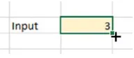
The second item is fulfilled when you store application variables on the worksheet. This is because the only way to change these variables is by either writing to them with code or updating them manually behind the scenes. Let’s say you have a named ranged called Calculate.Input. I can change this variable’s value in the code (see below), which requires I run a macro.

[Calculate.Input] = 1

Or I can change its value by finding it on the spreadsheet and typing in something new, as in Figure 2-19.

Figure 2-19. A worskheet named range variable called Calc.Input

However, if I want to access this variable somewhere else on the worksheet, I must access it through a formula, like this:

= Calc.Input – 1

Notice that this simply accesses the value stored in Calc.Input—it doesn’t change the value itself. However, it’s impossible with a formula to change the value of Calc.Input. Like I said above, there are only two ways to change its value, a macro or a human. This is an example of encapsulation.

The Last Word

(31)

Introducing Formula Concepts

Q: What does every newborn spreadsheet need?

A: Formula

Spreadsheet formulas hold a unique place in advanced Excel development. Most of us are familiar with formulas as a means to produce results more quickly than with manual calculation. For example, if we want to find the arithmetic sum of a range, does it make sense to pull out the Burroughs Adding Machine and punch in each item one by one? No. The very nature of a spreadsheet provides a built-in means to manipulate its elements.

Most of us are used to this type of manipulation with formulas; that is, we use formulas as a means to find and return results. Spreadsheet formulas, when used for Excel development, however, do much more. They form the infrastructure upon which much of our work is based.

Throughout this book we will be working with formulas. Some of these formulas will be very complex. When you first start, they may appear daunting. However, practice makes perfect, and experience is your greatest teacher. The more you use them, the more you develop a formula literacy. What may have appeared hard to read at first glance should become easier. But more important than knowing the formulas themselves is understanding the concepts behind what drives them.

And, of course, Excel includes a few tools and features to help you understand your formulas. Let’s go through a few of them you can start using now.

Formula Help

In this section, I’ll talk about making the most of your formula experience. The following tips should make your life easier, especially when working with complex formulas.

F2 to See the Formula of a Select Cell

(32)

CHAPTER 3 ■ INTRODUCING FORMULA CONCEPTS

Listing 3-1. An Example of a Long, Complex Formula

=IF(SUMPRODUCT(A1:A3*(B1:B3>2))>7, CONCATENATE(A2 & L3), IFERROR(C6, "An error occurred."))

Let’s say you want to evaluate only a part of this formula, specifically the highlighted portion of the same formula but now in Excel’s formula bar (Figure 3-1).

Figure 3-1. You can select a portion of the formula to be evaluated immediately

Figure 3-2. Pressing F9 on the highlighted portion evaluates the highlighted portion immediately

Figure 3-3. The Evaluate Formula button

In fact, you can tell Excel to evaluate just that easily. If you highlight the portion as I’ve done in Figure 3-1, you can press F9 to see what it evaluates to (see Figure 3-2).

You now see this portion evaluates to False. In the formula bar, Excel just rewrites this portion of highlighted text to read “FALSE.” And you can do this to any portion of the formula. If you click outside the formula bar or press the escape key, the formula will return to its original, unevaluated text. F9 then, when used with formulas, is the ultimate on-demand approach for quick formula evaluation.

Evaluate Formula Button

The Evaluate Formula button allows you to step through an entire formula. Here’s how it works. First, click the cell you’re interested in investigating. Then, click the Formulas tab on the ribbon. Go to Evaluate Formulas in the Formula Auditing group. Take a look at Figure 3-3.

(33)

Excel Formula Concepts

In this section, I’ll talk about formula concepts you’ll be using throughout the rest of this book. To begin, Excel formulas are made up of four main types:

Functions, such as

•฀ AVERAGE( ), SUM( ), IF( )

Constants and literals, such as number, string, and Boolean values like 2, 100, 1E7, •฀

You’re probably already familiar with several of these types. Obviously, functions make up a huge part of formula use. Constants that are numbers are also probably familiar. However, did you know that Boolean values like TRUE and FALSE are also constants? Finally, you’ve probably used references and operations many times by now, but did you know the colon (:) that forms the range A$1$:A$20$ is also an operator?

Operators, in Depth

This section will discuss Excel operators. You’re probably familiar with Excel’s arithmetic operators, plus (+), minus (-), times (*), and divide (/). But besides arithmetic operators, Excel has a text and three reference operators.

Excel’s text operator is the ampersand (&), which stands in for the CONCATENATE function. For instance, the formulas =A1&B1 and =CONCATENATE(A1,B1) do the exact same thing. You’ve probably also used Excel’s reference operators many times, the colon (:) in particular, without thinking of them as operators. Excel’s two other reference operators are the comma (,) and space ( ) characters. Table 3-1 talks about what they do.

(34)

In the next few sections, I’ll go through examples of what you can do with these reference operators.

The Range Operator (:)

In this section, I discuss the range operator. The range operator (:) is one of the most used operators in Excel. It’s an operator in every sense of the word in that it acts upon two different ranges (which are the operands, if you want to get technical) and returns a contiguous range. What’s so great about the range operator is that you can actually combine functions, like

= A1:INDEX(A:A, COUNTA(A:A))

and

= B1:OFFSET(B:B, COUNTA(B:B), 0)

So let’s take a look at an example that shows the power of the range operator.

EXAMPLE: DYNAMICALLY SIZED RANGES

Using the range operator, you can create dynamically sized ranges. This means you can create a range that can

grow and shrink as the list they represent is added to or subtracted from. Both the

INDEX

and

OFFSET

formulas

can help you with this mechanism. In this example, they both work about the same way.

Consider the range in Figure

3-5

.

Table 3-1. Reference Operators and Their Descritions

Reference Operator

Nomenclature

Definition

: (colon) Range operator Combines all cells between two ranges, and the two cells into one contiguous range.

, (comma) Union operator Combines multiple references into one reference.

(space) Intersection operator Returns only the overlapping cells of one or more ranges.

(35)

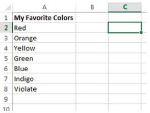
If I want a count of all my favorite colors in this example (in real life, I have only one favorite color, and

it’s black

), I can use the

COUNTA

function on the range A2 to A8. But what if I want to add to the list? In that case,

I must reapply my formula to accommodate the next color in cell A9. Alternatively, I can just say something like

A2:A1000

, where the second range is an arbitrarily large number. Neither the former’s formula reapplication nor

the latter’s arbitrarily high number are very good fixes.

The best solution is to use a dynamically sized range. To do this with the

INDEX

formula, you can write

=$A$2:INDEX($A:$A,COUNTA($A:$A))

like in Figure

3-6

.

Figure 3-6. A demonstration of the formula that will ultimately help you create a dynamically sized range

Here’s how it works. You supply the entire column range A:A to the

INDEX

formula. In the row argument of the

INDEX

formula, you’re interested in the last row of content in the column range of A:A.

COUNTA

, which counts

every filled cell in the range supplied to it, will return an 8, since the last row of content is the eighth row down.

When you use

INDEX

, you’re probably used to its returning values. If you hadn’t added that A1 at the beginning of

the formula, the

INDEX

function by itself would have simply returned the word “Violate.” But behind the scenes,

Excel is actually returning a

reference

to the cell containing “Violate,” not just its value. So, effectively, Excel is

returns A8, which becomes A1:A8 in the formula.

(36)

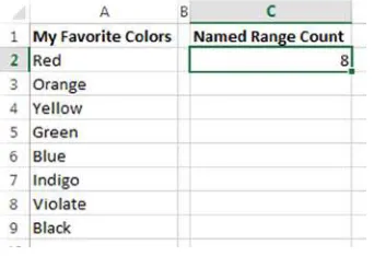
You can then use that named range elsewhere on your spreadsheet. For example, in cell C8 in Figure

3-8

, I’ve

used the formula

=COUNTA(myNamedRange)

. As you can see, I’ve added to my list, and the count has updated

automatically. Just imagine using these dynamically sized ranges in charts, dropdowns, and formulas! You’ll get

to do that in the next chapter.

Figure 3-8. Using the Name Range elsewhere

You can do the same with

OFFSET

, using this formula:

=$A$2:OFFSET($A$1,COUNTA($A:$A),0)

Experiment a little and see if you can figure this one out. Remember, if you need help, use the formula help

suggestions from the beginning of the chapter.

A final note is in order. There’s also some argument on whether

INDEX

is faster than

OFFSET

, since

OFFSET

is a

volatile function (that means it will recalculate every time the sheet recalculates) and

INDEX

is not. In general,

I prefer

INDEX

for this reason.

The Union Operator (,)

The union operator (,) is also likely familiar to you. The formula =SUM(A1:A10,C1:C5) employs the union operator to combine the two disparate ranges into one range upon which to take the sum. Unlike the range operator, which forms a contiguous range between two cells, the union operator essentially turns the two noncontiguous ranges into one long range. Think of it like this:

In this next section, I’ll talk about how you can use the union operation to your advantage. A1:A10 C1:C5

(37)

EXAMPLE: PULLING RANK

Let’s say you wanted to find where a certain number ranks within a series of numbers, when they’re ordered.

For example, if you have an unsorted series of numbers (8,4,6,1, and 2), you can use Excel’s

RANK

function to find

where the number 6 resides in a descending list of these numbers.

In Figure

3-9

, I have the formula

=RANK(D2,$A$2:$A$6)

in cell D2.

Figure 3-9. A demonstration of finding the rank of a given number within an unsorted list

8

6 4 1 2

Six is highlighted and is in the second place in the region.

Figure 3-10. A visual representation of how this example works

RANK

will automatically turn the range in the given series in descending order (by default, descending is selected;

however, this can be changed in

RANK’s

third, optional parameter). The rank of the number 6 then is 2, as shown

in Figure

3-10

.

This function only works when the input number (in D2 above) is a number in the set of the five given numbers.

But what if you want to find where the number 4.4 resides in the ordered series? The formula, left as is, will

return an NA( ) error if D2 is set to 4.4. To get around this, you need to add the input number to the set of

numbers. You can do this with the union operator, like so:

=RANK(D2,($A$2:$A$6,D2))

If D2 = 4.4, the series

($A$2:$A$6,D2)

becomes

8, 6,4.4, 4, 1, 2

, which returns the number 3. Consider

how this formula might be useful. If you have a list times, dates, or temperatures and want to return certain

information when an input value is between two boundaries, you can do that with this formula.

(38)

You’ll learn a creative use for the intersection operator in this next example.

INTERSECTING REGIONS AND MONTHS

Let’s say you have a table of units sold by month and region, like in Figure

3-12

.

Figure 3-12. A sample set of regional and monthly data

Figure 3-13. An application of the union operator on sample regional and monthly data

Figure 3-11. The intersection operator in action

To save time, you’ve had a macro assign columns B through H to be the named ranges Jan, Feb, Mar... etc. You’ve

done the same thing for each region, assigning the row ranges to North, South, East, and West.

(39)

The formula returns 1366, which is the sum of 201, 747, and 388. If you want to see the performance for the

eastern region for just the months of January and March but not February, you can use the following formula:

=SUM(East Jan + East March)

If you’re particularly mathematically minded, and hopefully you will be somewhat by the end of the next chapter,

you can simplify this formula like so:

=SUM(East (Jan, March))

Note that

East Jan + East March = East (Jan, March)

, which parallels the Distributive Law of algebra.

I’ll go into this in a little more detail later in the next chapter.

When to Use Conditional Expressions

In this section, you’re going to dive deeper into conditional expressions. If you’ve used IF, then you’ve used a conditional expression before. Conditional expressions are all about testing things. For example, in the formula =IF(AB>2, "Yes", "No"), the first argument, AB>2, is the conditional expression. Any expression that uses the logic operators, =, <, >, etc., is a conditional expression.

So you want to test the value of a cell and return a result if it passes a test or another result if it fails. Quick: which function should you use?

Was your answer IF? If it was, then you’re not alone. The IF function feels like a natural choice, especially because the first parameter of the IF function calls for a logical expression. But there are also some instances where IF isn’t the best choice. The Excel MVP, Daniel Ferry, has gone so far as to argue that the IF function is the most overused function of all. And, as this chapter will demonstrate, there’s good reason to believe this.

Deceptively Simple Nested IF Statements

One supposed advantage to using the IF function is the ability to make use of nesting conditions. For example, if I have multiple compounding conditions, I can place IF statements inside the value_if_true and value_if_false parameters (Listing 3-2). In my experience, however, IF statements are nested far more often than they need to be.

Listing 3-2. A Prototype of the IF Function

IF(logical_test, value_if_true, value_if_false)

Even I have to admit that nested IF statements are unavoidable. But I like to save them for formulas that exhibit natural branching conditions. Consider

=IF(ProjectStatus = "Stopped", IF(Err_Code=1, "Halted by internal error.","Uknown error."), "Project has NOT finished.")

(40)

Sometimes it’s not always so clear whether the problems represent a compound branching condition. A good rule of thumb is to start from one of the possible results and work backwards. Ask yourself: does the result naturally follow from the test condition? In other words: does this result make sense given the conditions?

Confused? I hear you. Well, let’s consider the following example from Microsoft’s very own help guide, shown in Listing 3-3.

Listing 3-3. An Example of Nested IFs from Microsoft’s Excel Help

=IF(A2>89,"A",IF(A2>79,"B", IF(A2>69,"C",IF(A2>59,"D","F"))))

This formula returns a letter grade based on a student’s raw grade stored in A2. It’s a good example of a problem that makes for a poor branching condition. The grade you receive isn’t the result of not receiving another grade. (I know you’re scratching your head here but bear with me for a moment). Your letter grade is the result of where your score falls within one of five different numerical boundaries. If anything, this is a lookup problem. You could easily employ the RANK function example from above or use the MATCH function. But if you were to frame this problem organically, the reason a student receives an F is not because they didn’t receive a D, C, B, or A. The IF function above turns this lookup problem into a branching condition problem when it needn’t be.

Another common example involves using states as numbers. Consider the formula in Listing 3-4.

Listing 3-4. Another Example Using IFs That Isn’t a Branching Condition

=IF(A2=1, "Small",IF(A2=2,"Med", "Large")).

(41)

In this example, A2 holds an encoded Id or state. For an example like this, the states could be anything, but they usually form some natural ordinal scale. In the example above, the Ids map to the following results: 1=Small, 2=Medium, and 3=Large. We call these categories ordinal because they can be ordered naturally. Here again, IF is not a good choice. The problem presented is not a branching condition but rather a test of scale. Indeed, for formulas like these, the CHOOSE function is a much better choice.

CHOOSE Wisely

In this section, I’ll go through how to use CHOOSE, and why for some situations it makes for a better choice than IF. CHOOSE is much like IF, but it can more naturally deal with ordinal data. Listing 3-5 includes the prototype for CHOOSE.

Listing 3-5. CHOOSE( ) Prototype

CHOOSE(index_num, value1, value2,...)

CHOOSE analyzes the argument supplied to the index_num parameter and returns the value at the given index number. In the example above, when index_num is 1, value1 is returned; when index_num is 2, value2 is returned, and so forth.

In the previous instance, you could simply write =CHOOSE(A2, "Small", "Med", "Large"). This appears to be more closely align with the way this example is naturally formulated. Because of this, CHOOSE makes the data arrangement more easy to read and understand at first glance. Compare the two arrangements:

IF arrangement

=IF(A2=1, "Small",IF(A2=2,"Med", "Large")).

CHOOSE arrangement

=CHOOSE(A2, "Small", "Med", "Large")

GENERATING RANDOM DATA WITH CHOOSE( )

CHOOSE

is also great for generating random categorical or nominal data. This type of random data generation

is particularly useful to create test data for your dashboard backend database. All it takes is the addition of the

RANDBETWEEN

function. Say you have categorical data of Big, Medium, and Little. You could generate data with the

following formula:

=CHOOSE(RANDBETWEEN(1,3), "Big", "Medium", "Little")

Why This Discussion Is Important

(42)

So then why have I made the distinction? Well, using the formula that best matches what you’re trying to accomplish just makes sense. In addition, and perhaps more importantly, when you come back to your formula later after having been away from your spreadsheet for a while, a formula that better matches your test conditions will ultimately be easier to once again comprehend, especially if it’s complex in nature.

Ok, you’re not convinced. I wasn’t at first, either. In the end, there may not be a noticeable difference between using IF or CHOOSE, I admit. But in the previous chapter I turned conventional coding on its head. And I’ll keep doing so throughout this book.

And if you’re tempted to keep using IF, read on. Chances are you’ll find it at least one example in which IF isn’t necessary.

Introduction to Boolean Concepts

In this section, I’ll talk about concepts surrounding Boolean expressions. For the unfamiliar, Boolean formulas use a type of mathematical logic called Boolean algebra and they’re the natural result of conditional expressions.

The most important feature of a Boolean expression is that it always returns one of two mutually exclusive values: either it returns TRUE, or it returns FALSE. Excel, however, brings another important twist to the TRUE/FALSE dynamic. Sometimes TRUE can also mean the number one, and FALSE can also mean the number zero. Let’s take a look in the following example.

FILTERING ODD OR EVEN VALUES

Booleans are great for filtering. Take a look at Figure

3-15

. In this example, I’ve created a mechanism to only

show either odd or even values in the accompanying chart.

(43)

I provide the user a dropdown box to select between either showing odd values or even values. On the left, I’ve

included a table that helps evaluate what the final chart will show. Figure

3-16

shows this table in more detail.

Figure 3-16. The table that allows for chart filtering

In column B, I use the following formula:

=CHOOSE(MOD(A3,2)+1,"Even","Odd")

So let’s break this down.

Nested inside the

CHOOSE

conditional is the

MOD( )

formula.

MOD

performs

modulo division

, which is a technical

way of saying it performs division like a third grader. Remember when you first started learning how to divide,

3 divided by 2

would equal

1 remainder 1

? Well, modulo division performs this same operation but only returns

the remainder part. In the case of

MOD(A3,2)

you’re simply testing whether the list of numbers given in column

A is odd or even. As you might recall, when even numbers are divided by two, there is never a remainder

(think of it as a reminder of zero); for odd numbers there’s always a remainder of one.

What you run into is that you’re using the

CHOOSE( )

formula to tell Excel whether to return the word “Odd,” or to

return the word “Even.”

CHOOSE( )

, however, can’t take in numbers that are less than one, and so far, it’s possible

this could return a zero. So, my solution is to add the one at the end. So going back to the original

CHOOSE

formula,

=CHOOSE(MOD(A3,2)+1,"Even","Odd")

...you can see how all the parts fit together.

(44)

This is achieved by writing the following Boolean formula from cell C3:

=(B3=$L$2)

The parentheses surround the test condition telling Excel to either return a TRUE or FALSE value. When there’s

only one test case, the parentheses are optional. However, it’s good practice to keep parentheses anyway, keeping

in line with the idea presented above that you should match your formulas to manifest the conditions you’re

developing. And, specifically, note that the following two formulas are not equal:

=(B3=$L$2)+1 =\= =B3=$L$2+1

Finally, in Column D you multiply columns A and C (Figure

3-18

). When the number in Column A is multiplied by

a

TRUE

value, it’s the same as multiplying it by the number one. When multiplied by a

FALSE

value, it’s the as

multiplying it by zero. The chart is linked to column D so the outcomes in column D are automatically updated on

the chart.

Figure 3-18. The Final Value column of your table

I have to admit: CHOOSE wasn’t the best function for the example above. By all accounts, if you were thinking I should have used IF instead, you wouldn’t have been off base. The values of "Even" and "Odd" aren’t ordinal. Numbers are either only even or odd. And I’m usually of the belief that the more natural the function mirrors the problem, the easier it is to comprehend. What makes the example above such a good IF problem is because the Boolean dynamic, that TRUE/FALSE = 1/0, goes both ways. Recall in your test for an even or odd value, the MOD function was returning either a zero or a one. You could have written =CHOOSE(MOD(A3,2)+1,"Even","Odd") as =IF(MOD(A3,2),"Odd","Even") which is reasonably easier to read, and it’s probably easier to comprehend when you come back to it later.

Condensing Your Work

What makes =IF(MOD(A3,2),"Odd","Even") so readable is because there are no nested conditions. Once you add more conditions, it becomes much harder to comprehend at first glance. And, when you represent information on your spreadsheet, you’ll sometimes have to condense formulas from different cells into one to save space. In the example above, if you want to condense your work, you can do something like this in column D:

(45)

But now the IF function is longer and harder to understand. Maybe it’s time you dispense with the IF function altogether. But how can you recreate the same conditions without using IF? Well, you can use the exclusive-or function, XOR, like this:

=XOR($L$2="Even",MOD(A3,2))*A3

Note

■

XOR

is available only in Excel 2013.

The Legend of XOR( )-oh

Technically, XOR is not pronounced “zore,” but rather as “ex-or,” which as you’ve likely figured is shorthand for exclusive-or. So what the heck does XOR do? Well it’s a type of truth-testing conditional function. You’re probably somewhat familiar with Excel’s cousin truth functions, AND and OR.

Let’s review them first. AND tests if all the supplied conditional expressions are TRUE. If they are, AND returns TRUE. If one condition is not true, as in FALSE, AND returns FALSE. OR tests if only one argument is TRUE and returns TRUE when at least one conditional expression evaluates to TRUE. If all arguments passed to OR evaluate to FALSE, OR returns FALSE. Table 3-2 shows the outcomes for AND and OR formulas when supplied with only two arguments, x and y.

Table 3-2. A Truth Table for AND and OR Functions

X

Y

=AND(x,y)

=OR(x,y)

XOR adds an extra constraint: only one of the arguments can contain a value of TRUE. That’s what makes it so

(46)

Going back to your condensed formula, let’s see how XOR( ) works by examining this formula:

=XOR($L$2="Even",MOD(A3,2))*A3.

Recall, MOD(A3,2) will return a one when A3 is odd and a zero when A3 is even. In the example above, you’re always testing if the dropdown has “Even” selected. So, let’s say A3 equals an odd value, like the number 3. Listing 3-6 shows a step-by-step evaluation when L2 is even. Listing 3-7 shows a step-by-step evaluation when L2 is odd.

Listing 3-6. Formula Evaluation When L2 Is Even

If $L$2="Even" then

Listing 3-7. Formula Evaluation When L2 Is Odd

If $L$2="Odd" then

So, think about this way: you’re actually interested in the inverse relationship between your two conditions. If $L$2 has "Even" selected, for the value in A3 to show, it must also be even. For even values, MOD(A3,2) will return a zero (which is the opposite result of the test $L$2 = "Even"). If $L$2 has "Odd" selected, the first argument will return FALSE, but MOD(A3,2) will actually return a one.

Do We Really Need IF?

For this section, I’ll combine everything you’ve learned so far to answer the question: do we really need IF? The fact is, many problems that feel like they need IF probably don’t need it. Let’s go through a few quick examples.

Need to test if a cell is blank so you can return a blank instead of a zero?

Use: =--REPT(A2, LEN(A2)>1) Instead of: IF(LEN(A2) > 1, A2, "")

Note: "--" is shorthand to convert a string into a number.

Need to return a certain range based on a dropdown select?

(47)

Use: =CHOOSE(--LEFT(A2, 1), NorthRange, EastRange, SouthRange, WestRange) Instead of: IF(A2 = "North", NorthRange, IF(A2 = "East", EastRange,

IF(A2 = "South", SouthRange, WestRange)

Want to know what grade you got?

Figure 3-20 shows a grade letter calculator.

Figure 3-19. Adding numbers to the dropdown items can help you quickly ascertain which item was selected without using an IF statement

Figure 3-20. A grade calculator that uses INDEX and MATCH instead of nested IFs

Figure 3-21. You can use Boolean functions instead of IF

Use: =INDEX($B$4:$B$8, MATCH(B1,$A$4:$A$8,1))

Instead of: = IF(B1>89,"A",IF(B1>79,"B", IF(B1>69,"C",IF(B1>59,"D","F"))))

Need to return a -1 whenever a test condition is zero; otherwise return the value?

(48)

The Last Word

I realize some of the material in this chapter might be new for you. And perhaps you’re not yet ready to turn your back on IF. Fair enough; although don’t expect me to use it much from here on out! The point of this chapter is to get your mind to think differently about certain problems. IF is a common convention, but the popular choice isn’t always the best. This chapter introduced you to formula concepts you’ve used many times before but might not have realized what they were or what they meant. Empowered with new knowledge, I’m confident you’ll be able to think about formulas differently.

(49)

Advanced Formula Concepts

The previous chapter’s formula examples may have appeared complicated at first, but you should be able to use them with time, practice, and patience. If you followed the advice at the start of Chapter 3, which was to work through formulas with techniques like Excel’s Evaluate Formula feature, you should find them easier to understand.

In this chapter, you will investigate how these formulas are applied. Specifically, I will cover the following:

Filtering and highlighting

Following what you learned about ones and zeros in Chapter 3, you can use formulas for filtering results. In Chapter 3, you employed a mechanism to filter even and odd values using Booleans. Highlighting, as it turns out, isn’t much different than filtering. Let’s take a look.

Filtering with Formulas

Figure 4-1 shows the tables I’ve set up for the example (download Chapter4Ex1.xlsx from the project files to follow along). If you have the example file open, we’re starting on the tab, Project List (incomplete). Throughout the example files, tabs with the suffix “(incomplete)” will refer to the unfinished work we’ll complete together. When available, tabs with the suffix “(complete)” will refer to completed versions I have built into the spreadsheet, so you can see what the final version looks like.

(50)

CHAPTER 4 ■ ADVANCED FORMULA CONCEPTS

Let’s take a better look at the table on the right. For the NPV column, let’s set up a conditional to compare whether the selected NPV is greater than the item in the current row of the Raw Data Table (Figure 4-2). Figure 4-1. An example table to demonstrate applied formula concepts

Figure 4-2. The Raw Data Table

Figure 4-3. You’re testing for what level of Portfolio Risk is selected