Low-Rank Doubly Stochastic Matrix Decomposition
for Cluster Analysis
Zhirong Yang [email protected]
Helsinki Institute of Information Technology HIIT University of Helsinki, Finland
Jukka Corander [email protected]
Department of Mathematics and Statistics
Helsinki Institute for Information Technology HIIT University of Helsinki, Finland
Department of Biostatistics, University of Oslo, Norway
Erkki Oja [email protected]
Department of Computer Science Aalto University, Finland
Editor:Maya Gupta
Abstract
Cluster analysis by nonnegative low-rank approximations has experienced a remarkable progress in the past decade. However, the majority of such approximation approaches are still restricted to nonnegative matrix factorization (NMF) and suffer from the following two drawbacks: 1) they are unable to produce balanced partitions for large-scale manifold data which are common in real-world clustering tasks; 2) most existing NMF-type cluster-ing methods cannot automatically determine the number of clusters. We propose a new low-rank learning method to address these two problems, which is beyond matrix factor-ization. Our method approximately decomposes a sparse input similarity in a normalized way and its objective can be used to learn both cluster assignments and the number of clus-ters. For efficient optimization, we use a relaxed formulation based on Data-Cluster-Data random walk, which is also shown to be equivalent to low-rank factorization of the doubly-stochastically normalized cluster incidence matrix. The probabilistic cluster assignments can thus be learned with a multiplicative majorization-minimization algorithm. Exper-imental results show that the new method is more accurate both in terms of clustering large-scale manifold data sets and of selecting the number of clusters.
Keywords: cluster analysis, probabilistic relaxation, doubly stochastic matrix, manifold, multiplicative updates
1. Introduction
The most popular nonnegative low-rank approximation method is Nonnegative Matrix Factorization (NMF; Lee and Seung, 1999, 2001). It finds a matrix which approximates the pairwise similarities between the data items and can be factorized into two nonnegative low-rank matrices. NMF was originally applied to vector data, for which Ding et al. (2010) did later show that it is equivalent to the classicalk-means method. NMF has also been applied to weighted graph defined by the pairwise similarities of the data items. For example, Ding et al. (2008) presented Nonnegative Spectral Cuts by using a multiplicative algorithm; and Arora et al. (2011, 2013) proposed Left Stochastic Decomposition that approximates a similarity matrix based on Euclidean distance and a left-stochastic matrix. Topic modeling represents another example of a related factorization problem. Hofmann (1999) introduced a generative model in Probabilistic Latent Semantic Indexing (PLSI) for counting data, which is essentially equivalent to NMF using Kullback-Leibler (KL) divergence and tri-factorizations. Bayesian treatment of PLSI by using Dirichlet priors was later introduced by Blei et al. (2001). Symmetric PLSI with the same Bayesian treatment is calledInteraction Component Model (ICM; Sinkkonen et al., 2008).
Despite the remarkable progress, the above NMF-type clustering methods still suffer from one or more of the following problems: 1) they are not accurate for the data in curved manifolds; 2) they cannot guarantee balanced partitions; 3) their learning objectives cannot be used to choose the number of clusters. The first problem is common in many real-world clustering tasks, where data are represented by raw features and simple similarity metrics such as Euclidean or Hamming are only accurate in small neighborhoods. This induces sparse accurate similarity information (e.g. as with the K-Nearest-Neighbor for a relatively small K) as input for clustering algorithms. In the big data era, the sparsity is also necessary for computation efficiency for large amounts of data objects. Most existing clustering methods, however, do not handle well the sparse similarity. The second problem arises due to the lack of suitable normalization of partitions in the objective function. Consequently, the resulting cluster sizes can be drastically and spuriously variable, which hampers the general reliability of the methods for applications. The third problem forces users to manually specify the number of clusters or to rely on external clustering evaluation methods which are usually inconsistent with the used learning objective.
In this paper we propose a new clustering method that addresses all the above-mentioned problems. Our learning objective is to minimize the discrepancy between the similarity matrix and the doubly-stochastically normalized cluster incidence matrix, which ensures balanced clusterings. Different from conventional squared Euclidean distance, the discrep-ancy in our approach is measured by Kullback-Leibler divergence which is more suitable for sparse similarity inputs. Minimizing the objective over all possible partitions automatically returns the most appropriate number of clusters.
We also propose an efficient and convenient algorithm for optimizing the introduced objective function. First, by using a new nonnegative matrix decomposition form, we find an equivalent solution space of low-rank nonnegative doubly stochastic matrices. This provides us a probabilistic surrogate learning objective called Data-Cluster-Data (DCD in short). Next we develop a new multiplicative algorithm for this surrogate function by using the majorization-minimization principle.
clusterings, especially for large-scale manifold data sets containing up to hundreds of thou-sands of samples. We also demonstrate that it can select the number of clusters much more precisely than other existing approaches.
Although a preliminary version of our method has been presented earlier (Yang and Oja, 2012a), the current paper introduces several significant improvements. First, we show that the proposed clustering objective can be used to learn not only the cluster assignments but also the number of clusters. Second, we show that the proposed structural decomposition is equivalent to the low-rank factorization of a doubly stochastic matrix. Previously it was known that the former is a subset of the latter and now we prove that the reverse also holds. Third, we have performed much more extensive experiments, where the results further consolidate our conclusions.
The remainder of the paper is organized as follows. We review the basic clustering objective in Section 2. Its relaxed surrogate, the DCD learning objective, as well as opti-mization algorithm, are presented in Section 3, and the experimental results in Section 4, respectively. We discuss related work in Section 5 and conclude the paper by presenting possible directions for future research in Section 6.
2. Normalized Output Similarity Approximation Clusterability
Given a set of data objects X ={x1, . . . , xN}, cluster analysis assigns them into r groups, called clusters, so that the objects in the same cluster are more similar to each other than to those in the other clusters. The cluster assignments can be represented by acluster indicator matrix F¯ ∈ {0,1}N×r, where ¯F
ik = 1 if xi is assigned to the cluster Ck, and ¯Fik = 0 otherwise. The cluster incidence matrix is defined as ¯M = ¯FF¯T. Then ¯M ∈ {0,1}N×N and ¯Mij = 1 iff xi and xj are in the same cluster.
Let Sij ≥0 be a suitably normalized similarity measure between xi and xj. For a good clustering, it is natural to assume that the matrixSshould be close to the cluster incidence matrix ¯M. Visually, ¯M is a blockwise matrix if we sort the data by their cluster assignment, and S should be nearly blockwise. The discrepancy or approximation error betweenS and
¯
M can be measured by a certain divergenceD(S||M¯), e.g. Euclidean distance or Kullback-Leibler divergence. For example, He et al. (2011); Arora et al. (2011, 2013) used D(S||M¯) with Euclidean distance to derive their respective NMF clustering methods.
Directly minimizing D(S||M¯) can yield imbalanced partitions (see e.g., Shi and Malik, 2000). That is, some clusters are automatically of much smaller size than others, which is undesirable in many real-world applications. To achieve a balanced clustering, one can normalize ¯M to M in the approximation such that PNi=1Mij = 1 and PNj=1Mij = 1, or
equivalently by normalizing ¯F to F with Fik = ¯Fik/qPNv=1F¯vk. The matrix M = F FT then becomes doubly stochastic. Such normalization has appeared in different clustering approaches (e.g., Ding et al., 2005; Shi and Malik, 2000). In this way, each cluster in M
has unitary normalized volume (the ratio between sum of within-cluster similarities and the cluster size; also called normalized association (Shi and Malik, 2000)).
an easy reference within this paper, we call itNormalized Output Similarity Approximation Clusterability (NOSAC) and D(S||M) the NOSAC residual for a specific clustering M. Note that the optimum is taken over partitions which possibly have different values of r. Therefore the optimization can be used to learn not only cluster assignments but also the number of clusters. Similarly, minimizingD(S||M) can also be used to select an optimum among partitions produced by e.g. different hyper-parameters or different initializations.
Minimizing D(S||M¯) orD(S||M) is equivalent to a combinatorial optimization problem in discrete space which is typically a difficult task (see e.g. Aloise et al., 2009; Mahajan et al., 2009; Shi and Malik, 2000). In practice it is customary to first solve a relaxed surrogate problem in continuous space and then perform discretization to obtain ¯F or F. Different relaxations include, for example, nonnegative matrices (Ding et al., 2008; Yang and Oja, 2010) and stochastic matrices Arora et al. (2011, 2013) for the unnormalized indicator ¯F
in D(S||M¯), and orthogonal matrices (Shi and Malik, 2000), as well as nonnegative and orthogonal matrices (Ding et al., 2006; Yang and Oja, 2012b; Yang and Laaksonen, 2007; Yoo and Choi, 2008; Pompili et al., 2013) for the normalized indicatorF inD(S||M).
In this paper we emphasize that the doubly stochasticity constraint is essential for balanced clustering, which cannot be guaranteed by the above relaxations. Besides this constraint, we also keep the nonnegativity constraint to achieve sparser low-rank factorizing matrix. These conditions as a whole provide a tighter relaxed solution space AforM:
A=
To our knowledge, however, there is no existing technique that can minimize a generic cost function over low-rank A or over U. The major difficulty arises because the doubly stochasticity constraint is indirectly coupled with the factorizing matrixU. Note that this optimization problem is different from normalizing the input similarity matrix to be doubly stochastic before clustering (Zass and Shashua, 2006; He et al., 2011; Wang et al., 2012).
3. Low-rank Doubly Stochastic Matrix Decomposition by Probabilistic Relaxation
In this section we show how to minimize D(S||A) over A ∈ A with suitable choice of discrepancy measure and complexity control. First we identify an equivalent solution space of A which is easier for optimization. Then we develop the multiplicative minimization algorithm for finding a stationary point of the objective function.
3.1 Probabilistic relaxation
We find an alternative solution space by relaxingM to another matrix B in the matrix set
B=
Theorem 1 A=B.
The proof is given in Appendix A. Previously it was known that A ⊇ B (Yang and Oja, 2012a). Now this theorem shows thatA⊆Balso holds, which implies that we do not miss any solution inAby usingB. We preferBbecause the minimization inBis easier, as there is no explicit doubly stochasticity constraint and we can work with the right stochastic matrix W. Note that W appears in both the numerator and denominator within the sum overk. Therefore this structural decomposition goes beyond conventional nonnegative matrix factorization schemes.
A probabilistic interpretation of B is as follows. LetWik = P(k|i), the probability of assigning theith data object to thekth cluster.1 In the following,i,j, andvstand for data sample indices (from 1 toN) whilekandlstand for cluster indices (from 1 to r). Without preference to any particular sample, we impose a uniform priorP(j) = 1/N over the data samples. With this prior, we can compute
P(j|k) = PrP(k|j)P(j) v=1P(k|v)P(v)
= PrP(k|j) v=1P(k|v)
(3)
by the Bayes’ formula. Then we can see that
Bij = r X
k=1
WikWjk PN
v=1Wvk
(4)
= r X
k=1
P(k|j) PN
v=1P(k|v)
P(k|i) (5)
= r X
k=1
P(j|k)P(k|i) (6)
=P(j|i). (7)
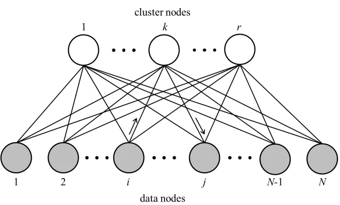
That is, if we define a bipartite graph with the data samples and clusters as graph nodes,
Bij is the probability that the ith data node reaches the jth data node via a cluster node (see Figure 1). We thus call this DCD random walk or DCD decomposition after the Data-Cluster-Data walking paths. Since B is nonnegative and symmetric (which follows easily from the definition), in non-trivial cases it can be seen as another similarity measure between data objects. Our learning target is to find a good approximation between the input similarity matrix S and the low-rank output similarity B.
3.2 Kullback-Leibler divergence
Euclidean distance or Frobenius norm is a conventional choice for the discrepancy measure
D. However, it is improper for many real-world clustering tasks where the raw data features are weakly informative. Similarities calculated with most simple metrics such as Euclidean distance or Hamming distance are then only accurate in a small neighborhood, whereas data
1. We use the abbreviation to avoid excessive notation. In full,P(k|i)def= P(β=Ck|ξ=xi), whereβandξ are random variables with possible outcomes in clusters{Ck}rk=1and data samples{xi}Ni=1, respectively.
SimilarlyP(i)def= P(ξ=xi) andP(i|k) def
Figure 1: Data-cluster bipartite graph for N data samples and r clusters (r < N). The arrows show a Data-Cluster-Data (DCD) random walk path, which starts at the
ith data node (sample) and ends at the jth data node via the kth cluster node.
points from different clusters often become mixed in wider neighborhoods. That is, only a small fraction of similarities, e.g. K-Nearest-Neighbor similarities with a relatively small value of K, are reliable and should be fed as a sparse input to clustering algorithms, while the similarities between the other, non-neighboring samples are set to zero. Least-square fitting with such a sparse similarity matrix is dominated by the approximation to the many zeros, which typically yields only poor or mediocre clustering results.
Here we propose to use (generalized) Kullback-Leibler divergence which is a more suit-able approximation error measure between the sparse input similarity S and the dense output similarityB, because the approximation relies more heavily on the large values inS
(see e.g. F´evotte and Idier, 2011). The underlying Poisson likelihood models more appropri-ately the rare occurrences of reliable similarities. We thus formulate our learning objective in the relaxed DCD space as the following optimization problem:
minimize
W≥0 DKL(S||B) = N X
i=1 N X
j=1
Sijlog Sij
Bij
−Sij+Bij
(8)
subject to Bij = r X
k=1
WikWjk P
vWvk
, (9)
r X
k=1
Dropping the constant terms in DKL(S||B), the objective function is equivalent to maxi-mizing PNi=1PNj=1SijlogBij because PNi=1
PN
j=1Bij =N. Note that this form is similar to PLSI (Hofmann, 1999) except for the decomposition form inB. Therefore we can enjoy the similar complexity control by using a Dirichlet prior (see Section 3.3).
Kullback-Leibler divergence also facilitates optimization, as we shall see in the algorithm development below. In objective and gradient calculation, it is straightforward to involve only the non-zero entries in S which brings an efficient implementation. Moreover, given properties of the logarithm function, we can break the comprehensive structure of B into several additive terms when majorizing the objective with the convex-concave procedure (Hunter and Lange, 2004). As a result, this yields relatively simple update rules in the algorithm. See Section 3.4 and Appendix B for details.
3.3 Regularization
The DCD learning objective function is parameterized by the matrix W whose rows sum to one. Assuming that these rows are observations from a common Dirichlet distribution, we can apply the log-Dirichlet prior to control the complexity in W. This gives the cost function of our DCD clustering method:
J(W) =− N X
i=1 N X
j=1
SijlogBij −(α−1) N X
i=1 r X
k=1
logWik. (11)
This is also equivalent to regularization by using a total Shannon information term. If Sij are integers, the DCD objective is the log-likelihood of the following generative model: 1) draw the rows of W according to uniform Dirichlet distribution with parameter
α; 2) for t= 1, . . . , T, add one to entry (i, j) ∼Multinomial N1B,1. The Dirichlet prior vanishes whenα = 1. By using α >1, the prior gives further relaxation by smoothing the
W entries, which is often desired in early stages of W learning.
Although it is possible to construct a multi-level graphical model similar to the Dirichlet process topic model (Blei et al., 2001; Sinkkonen et al., 2008), we emphasize that the smallest approximation error (i.e. withα= 1) is the final DCD goal. The Dirichlet prior is used only in order to ease the optimization. Therefore we do not employ more complex generative models.
3.4 Optimization
Multiplicative updates are widely used in optimization for nonnegative matrix factorization problems. To minimize an objective J over a nonnegative matrix W, we first calculate the gradient and separate it into two nonnegative parts (∇+ik ≥0 and∇−ik≥0):
∇ikdef=
∂J
∂Wik
=∇+ik− ∇−ik. (12)
Usually the separation can easily be identified from the gradient. Then the algorithm iteratively applies a multiplicative update rule Wik ← Wik
∇−
ik
W and do not require extra effort to tune learning step size. For a variety of NMF problems, such multiplicative updates monotonically decreaseJ after each iteration and thereforeW
can converge to a stationary point (Yang and Oja, 2011).
We cannot directly apply the above multiplicative fixed-point algorithm to DCD because there are probability constraints on theW rows. In practice, projecting theW rows to the probability simplex after each iteration would often lead to poor clustering result.
Instead, we employ a relaxing strategy (Zhu et al., 2013) to handle the probability constraint. We first introduce Lagrangian multipliers{λi}Ni=1 for the constraints:
L(W, λ) =J(W) +X
This suggests a preliminary multiplicative update rule for W:
Wik′ =Wik
Putting thisλback in Eq. 14, we obtain
Wik ←Wik
∇−ikai+ 1−bi ∇+ikai
. (18)
To maintain the positivity of W, we addbi to both the numerator and denominator, which does not change the fixed point and gives the ultimate update rule:
Wik ←Wik
∇−ikai+ 1 ∇+ikai+bi
. (19)
The above calculation steps are summarized in Algorithm 1. In implementation, one does not need to construct the whole matrixB. The ratioZij =Sij/Bij only requires calculation on the non-zero entries ofS.
Algorithm 1 Relaxed MM Algorithm for DCD
Input: similarity matrixS, number of clustersr, positive initial guess ofW. Output: cluster assigning probabilities W.
repeat
Bij = r X
k=1
WikWjk P
vWvk
Zij =Sij/Bij
sk =PNv=1Wvk
∇−ik = 2 (ZW)iks−k1+αWik−1
∇+ik = WTZWkks−k2+Wik−1 ai =
r X
l=1
Wil
∇+il, bi= r X
l=1
Wil ∇−il ∇+il
Wik ←Wik
∇−ikai+ 1 ∇+ikai+bi
until W converges under the given tolerance
Theorem 2 DenoteWnew
the updated matrix after each iteration of Algorithm 1. It holds thatL(Wnew
, λ)≤ L(W, λ) withλi = (bi−1)/ai.
The proof (given in Appendix B) mainly follows the Majorization-Minimization procedure (Hunter and Lange, 2004; Yang and Oja, 2011). The theorem shows that Algorithm 1 jointly minimizes the approximation error and drives the rows ofW towards the probability simplex. The Lagrangian multipliers are adaptively and automatically selected by the algorithm, without extra human tuning effort. The quantities bi are the row sums of the unconstrained multiplicative learning result, while the quantities ai balance between the gradient learning force and the probability simplex attraction. Besides convenience, we find that this relaxation strategy works more robustly than the brute-force projection after each iteration.
DCD minimizes the relaxed NOSAC residual for a particular r. To select the best number of clusters, we can run Algorithm 1 over a range ofrvalues, discretize W to obtain the hard cluster assignment ¯F, and return the one with smallest NOSAC residual. See Section 4.2 for examples.
3.5 Initialization
In particular, the regularized DCD (i.e. with various α6= 1) can also provide initializa-tion for the non-regularized DCD (i.e. withα= 1). That is, the parameter α only appears in the initialization and its best value is also determined by the smallest resultingD(S||M).
4. Experiments
We have tested the DCD method and compared it with other existing cluster analysis approaches. The experiments were organized in two groups: 1) we ran the methods with a fixed number of clusters, mainly comparing their clustering accuracies; 2) we ran DCD across different r values, demonstrating how to use NOSAC residual to determine the optimal number of clusters as well as its advantage over several other clustering evaluation methods.
4.1 Clustering with known number of clusters
In the first group of experiments, the number of the ground truth classes in the data sets was known in advance, and we fixedr to that number. We compared DCD with a variety of state-of-the-art clustering methods, including Projective Nonnegative Matrix Factorization (PNMF; Yang et al., 2007; Yang and Oja, 2010), Nonnegative Spectral Clustering (NSC; Ding et al., 2008), Orthogonal Nonnegative Matrix Factorization (ONMF; Ding et al., 2006), Probabilistic Latent Semantic Indexing (PLSI; Hofmann, 1999), Left-Stochastic Decomposi-tion (LSD; Arora et al., 2011, 2013), as well as two classical methods k-means (Lloyd, 1982) and Normalized Cut (Ncut; Shi and Malik, 2000). Besides NMF, we have also selected several recent clustering methods, including 1-Spectral (1-Spec; Hein and B¨uhler, 2010), Landmark-based Spectral Clustering (LSC; Chen and Cai, 2011; Cai and Chen, 2015), Sparse Subspace Clustering (SSC; Elhamifar and Vidal, 2009, 2013), and Multiclass Total Variation (MTV; Bresson et al., 2013). There are some other recent methods (e.g., Ro-driguez and Laio, 2014; Liu and Tao, 2016), which is however not scalable to large numbers of samples and thus not included here.
We used default settings in the compared methods. The NMF-type methods were run with maximum 10,000 iterations of multiplicative updates and with convergence tolerance 10−6. We used ratio Cheeger cut for 1-Spec. All methods except k-means, Ncut, 1-Spec, LSC, SSC, and MTV were initialized by Ncut. That is, their starting point was the Ncut cluster indicator matrix plus a small constant 0.2 to all entries.
We have compared the above methods on 43 data sets from various domains, including biology, image, video, text, remote sensing, etc. All data sets are publicly available on the Internet. The data sources and statistics are given in the supplemental document. For similarity-based clustering methods, we constructed K-Nearest-Neighbor graphs from the multivariate data withK = 10. The adjacency matrices of the graphs are then symmetrized and binarized to obtainS, i.e. Sij = 1 ifxj is one of the K nearest neighbors ofxi or vice versa; otherwiseSij = 0. This produces sparse similarity matrices.
We have used two performance measures for the clustering accuracies: the first iscluster purity which equals N1 Prk=1max1≤l≤rnkl, where nkl is the number of data samples in the clusterkthat belong to ground-truth classl; the second performance measure isNormalized Mutual Information (NMI, Vinh et al., 2010) which equalsPrk=1Prl=1 nkl
N log nkl/N
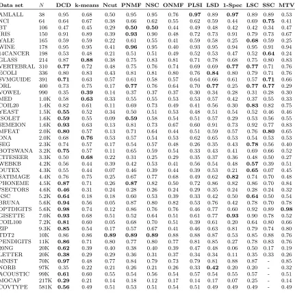
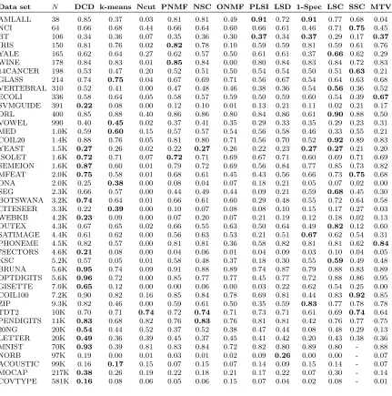
The resulting cluster purities and NMIs are shown in Tables 1 and 2, respectively. We can see that our method has much better performance than the other methods. DCD shows the optimal performance for 22 and 18 out of 43 data sets in purity and NMI, respectively, which is substantially more frequently than for any of the other methods. Even for some other data sets where DCD is not the winner, its cluster purities still remain close to the best method. Our method shows particularly superior performance when the number of samples grows. For the 19 data sets with N >4500, DCD is the top performer in 17 and 11 cases in purity and NMI, respectively. Note that purity corresponds to classification accuracy up to a permutation between classes and clusters. In this sense, our method achieves accuracy very close to many modern supervised approaches for some large-scale data in a curved manifold such asMNIST2, though our method does not use any class labels. For text document data set 20NG, DCD achieves comparable accuracy to those with comprehensive feature engineering and supervised classification (e.g. Srivastava et al., 2013), even though our method only uses simple bag-of-words Tf-Idf features and no class labels at all.
4.2 Selecting the number of clusters
In the second group of experiments, we assume that the number of clusters is unknown and it must be automatically selected from a range around the number of ground truth classes. We ran DCD with different values of r and calculated the corresponding NOSAC residual after discretizing W to cluster indicator matrix; the best number of clusters was then selected by ther with the smallest NOSAC residual.
We have compared the above DCD selection method with several other clustering eval-uation methods: Calinski-Harabasz (CH; Calinski and Harabasz, 1974), Davies-Bouldin (DB; Davies and Bouldin, 1979) and gap statistics (Tibshirani et al., 2001). We used their implementation in Matlab. Each cluster evaluation approach comes with a supported base clustering algorithm k-means (km) or linkage (lk). We thus have in total six methods for selecting the number of clusters to be compared against DCD. Some of these compared methods are very slow and required computation of more than five days for certain data sets. This drawback is especially severe for data sets with very high dimensionality such as
CURETand COIL100. In contrast, DCD required at most two hours for any tested data set.
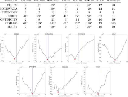
The results are reported in Table 3, which shows that DCD performs the best also in terms of selecting the number of clusters. The corresponding curves of NOSAC residual vs. number of clusters by DCD are shown in Figure 2. In the selected number of clusters, the DCD results are closest to the ground truth for all data sets, much more accurately than for any of the other methods. DCD correctly selects the best for CURET,OPTDIGITS, and
MNIST, and almost correctly (only differing by 1) for BOTSWANA and PHONEME. For COIL20
and COIL100, the DCD results are also reasonably good because we did not deliberately tune the extent of the local neighborhoods. By simply replacing 10NN with 5NN as the input similarities, DCD respectively selects 21 for COIL20and 99 for COIL100 as the best number of clusters.
Table 1: Clustering purities for the compared methods on various data sets. Boldface num-bers indicate the best in each row. “-” means out-of-memory error.
Data set N DCD k-means Ncut PNMF NSC ONMF PLSI LSD 1-Spec LSC SSC MTV
AMLALL 38 0.95 0.68 0.50 0.95 0.95 0.76 0.97 0.89 0.97 0.89 0.89 0.53 NCI 64 0.64 0.67 0.38 0.66 0.62 0.55 0.62 0.59 0.44 0.69 0.75 0.41 BT 106 0.47 0.45 0.29 0.50 0.50 0.44 0.49 0.48 0.42 0.42 0.34 0.47 IRIS 150 0.91 0.89 0.39 0.93 0.90 0.48 0.72 0.73 0.91 0.79 0.73 0.67 YALE 165 0.59 0.59 0.22 0.61 0.55 0.41 0.59 0.58 0.25 0.68 0.59 0.25 WINE 178 0.95 0.95 0.41 0.96 0.95 0.40 0.93 0.95 0.94 0.95 0.91 0.94 14CANCER 198 0.53 0.48 0.21 0.51 0.51 0.49 0.52 0.53 0.47 0.52 0.64 0.24 GLASS 214 0.87 0.88 0.38 0.75 0.83 0.81 0.71 0.78 0.68 0.75 0.80 0.83 VERTEBRAL 310 0.77 0.72 0.48 0.75 0.76 0.74 0.69 0.69 0.77 0.77 0.71 0.76 ECOLI 336 0.80 0.83 0.43 0.81 0.81 0.80 0.76 0.84 0.80 0.79 0.71 0.76 SVMGUIDE 391 0.71 0.63 0.57 0.61 0.58 0.57 0.64 0.66 0.61 0.57 0.71 0.66
ORL 400 0.73 0.75 0.17 0.77 0.76 0.64 0.70 0.77 0.25 0.77 0.77 0.29
VOWEL 990 0.35 0.39 0.14 0.37 0.37 0.37 0.30 0.34 0.28 0.31 0.28 0.30 MED 1.0K 0.58 0.63 0.33 0.55 0.55 0.53 0.53 0.57 0.42 0.37 0.55 0.33 COIL20 1.4K 0.82 0.61 0.11 0.69 0.73 0.49 0.41 0.56 0.30 0.83 0.82 0.75 YEAST 1.5K 0.55 0.52 0.34 0.50 0.51 0.53 0.48 0.51 0.54 0.52 0.46 0.46 ISOLET 1.6K 0.59 0.55 0.09 0.59 0.58 0.54 0.51 0.57 0.29 0.53 0.56 0.55 SEMEION 1.6K 0.93 0.63 0.13 0.81 0.73 0.67 0.60 0.91 0.73 0.92 0.77 0.83 MFEAT 2.0K 0.80 0.57 0.13 0.71 0.64 0.44 0.51 0.59 0.57 0.76 0.80 0.65 DNA 2.0K 0.68 0.76 0.53 0.57 0.54 0.53 0.62 0.65 0.53 0.54 0.53 0.53 SEG 2.3K 0.74 0.57 0.17 0.54 0.57 0.48 0.26 0.35 0.43 0.78 0.56 0.40 BOTSWANA 3.2K 0.75 0.57 0.11 0.65 0.59 0.54 0.33 0.43 0.41 0.69 0.66 0.52 CITESEER 3.3K 0.50 0.68 0.22 0.31 0.25 0.29 0.35 0.37 0.36 0.48 0.50 0.27 WEBKB 4.2K 0.56 0.44 0.39 0.42 0.53 0.41 0.56 0.54 0.48 0.57 0.39 0.51 OUTEX 4.3K 0.55 0.44 0.07 0.46 0.39 0.44 0.39 0.53 0.21 0.65 0.07 0.45 SATIMAGE 4.4K 0.76 0.75 0.25 0.67 0.77 0.68 0.49 0.62 0.82 0.74 0.70 0.48 PHONEME 4.5K 0.87 0.71 0.26 0.87 0.82 0.50 0.72 0.86 0.82 0.86 0.70 0.84 7SECTORS 4.6K 0.46 0.31 0.24 0.28 0.26 0.24 0.29 0.35 0.24 0.28 0.24 0.32 KSC 5.2K 0.64 0.18 0.18 0.60 0.53 0.39 0.33 0.42 0.50 0.64 0.50 0.54 BRUNA 5.6K 0.94 0.56 0.05 0.87 0.80 0.82 0.53 0.76 0.42 0.78 0.70 0.78 OPTDIGITS 5.6K 0.98 0.74 0.12 0.86 0.76 0.76 0.46 0.77 0.60 0.92 0.89 0.98
GISETTE 7.0K 0.93 0.68 0.51 0.52 0.64 0.51 0.61 0.77 0.93 0.90 0.78 0.52 COIL100 7.2K 0.81 0.60 0.05 0.68 0.70 0.51 0.39 0.61 0.20 0.64 0.80 0.66 ZIP 9.3K 0.85 0.54 0.17 0.57 0.67 0.41 0.46 0.63 0.81 0.79 0.74 0.80 TDT2 10K 0.86 0.86 0.89 0.89 0.89 0.88 0.88 0.87 0.53 0.85 0.88 0.76 PENDIGITS 11K 0.86 0.71 0.80 0.77 0.80 0.77 0.81 0.85 0.27 0.78 0.83 0.76 20NG 20K 0.62 0.39 0.40 0.38 0.40 0.39 0.47 0.48 0.06 0.50 0.17 0.19 LETTER 20K 0.38 0.29 0.29 0.36 0.31 0.37 0.34 0.34 0.11 0.35 0.33 0.26 MNIST 70K 0.97 0.48 0.77 0.84 0.79 0.73 0.79 0.81 0.88 0.87 - 0.85 NORB 97K 0.35 0.22 0.21 0.26 0.21 0.26 0.33 0.42 0.20 0.20 - 0.32 ACOUSTIC 99K 0.61 0.60 0.55 0.54 0.56 0.54 0.57 0.54 0.55 0.57 - 0.51 MOCAP 217K 0.29 0.21 0.14 0.18 0.12 0.17 0.14 0.17 0.07 0.25 - 0.14 COVTYPE 581K 0.56 0.49 0.51 0.53 0.51 0.54 0.51 0.49 0.49 0.49 - 0.49
5. Discussion
Table 2: Clustering NMIs for the compared methods on various data sets. Boldface numbers indicate the best in each row. “-” means out-of-memory error.
Data set N DCD k-means Ncut PNMF NSC ONMF PLSI LSD 1-Spec LSC SSC MTV
AMLALL 38 0.85 0.37 0.03 0.81 0.81 0.49 0.91 0.72 0.91 0.77 0.68 0.04 NCI 64 0.66 0.68 0.44 0.66 0.64 0.60 0.66 0.61 0.46 0.71 0.75 0.45 BT 106 0.34 0.36 0.07 0.35 0.36 0.30 0.37 0.34 0.37 0.29 0.17 0.37
IRIS 150 0.81 0.76 0.02 0.82 0.78 0.10 0.59 0.59 0.81 0.59 0.61 0.76 YALE 165 0.62 0.64 0.27 0.62 0.57 0.50 0.61 0.61 0.37 0.66 0.62 0.29 WINE 178 0.84 0.83 0.01 0.85 0.84 0.00 0.80 0.84 0.83 0.84 0.72 0.83 14CANCER 198 0.53 0.47 0.20 0.52 0.51 0.50 0.54 0.54 0.50 0.51 0.63 0.21 GLASS 214 0.74 0.75 0.04 0.67 0.69 0.71 0.56 0.67 0.54 0.64 0.63 0.68 VERTEBRAL 310 0.52 0.41 0.00 0.47 0.48 0.46 0.38 0.36 0.54 0.56 0.36 0.52 ECOLI 336 0.58 0.64 0.05 0.58 0.57 0.59 0.50 0.59 0.60 0.54 0.39 0.67
SVMGUIDE 391 0.22 0.08 0.00 0.12 0.10 0.01 0.13 0.21 0.11 0.02 0.21 0.17 ORL 400 0.85 0.88 0.40 0.86 0.86 0.80 0.84 0.86 0.61 0.90 0.88 0.50 VOWEL 990 0.40 0.45 0.02 0.37 0.41 0.35 0.29 0.33 0.35 0.29 0.23 0.31 MED 1.0K 0.59 0.60 0.15 0.57 0.57 0.54 0.56 0.58 0.46 0.33 0.55 0.21 COIL20 1.4K 0.88 0.76 0.05 0.81 0.80 0.71 0.56 0.70 0.52 0.92 0.89 0.83 YEAST 1.5K 0.27 0.26 0.02 0.22 0.27 0.26 0.22 0.23 0.27 0.27 0.21 0.20 ISOLET 1.6K 0.72 0.71 0.07 0.72 0.71 0.69 0.67 0.71 0.60 0.69 0.71 0.69 SEMEION 1.6K 0.87 0.60 0.01 0.79 0.72 0.69 0.56 0.84 0.77 0.85 0.73 0.82 MFEAT 2.0K 0.75 0.58 0.01 0.68 0.61 0.45 0.43 0.56 0.66 0.73 0.75 0.68 DNA 2.0K 0.25 0.38 0.00 0.08 0.04 0.07 0.18 0.21 0.05 0.07 0.02 0.00 SEG 2.3K 0.66 0.57 0.00 0.44 0.49 0.44 0.09 0.21 0.59 0.68 0.45 0.30 BOTSWANA 3.2K 0.74 0.64 0.01 0.66 0.61 0.60 0.29 0.48 0.55 0.72 0.64 0.58 CITESEER 3.3K 0.22 0.39 0.00 0.10 0.07 0.08 0.08 0.10 0.15 0.17 0.27 0.03 WEBKB 4.2K 0.23 0.09 0.00 0.07 0.20 0.07 0.21 0.19 0.12 0.18 0.02 0.13 OUTEX 4.3K 0.67 0.65 0.02 0.66 0.55 0.63 0.50 0.64 0.49 0.82 0.12 0.60 SATIMAGE 4.4K 0.61 0.62 0.00 0.56 0.63 0.53 0.21 0.51 0.67 0.62 0.54 0.31 PHONEME 4.5K 0.82 0.57 0.00 0.81 0.81 0.36 0.58 0.82 0.81 0.81 0.62 0.84
7SECTORS 4.6K 0.21 0.08 0.00 0.04 0.06 0.01 0.04 0.09 0.03 0.10 0.04 0.05 KSC 5.2K 0.57 0.05 0.01 0.58 0.48 0.37 0.18 0.30 0.55 0.59 0.49 0.48 BRUNA 5.6K 0.95 0.74 0.09 0.91 0.88 0.89 0.74 0.87 0.79 0.88 0.83 0.89 OPTDIGITS 5.6K 0.96 0.72 0.00 0.85 0.77 0.77 0.45 0.77 0.72 0.88 0.86 0.95 GISETTE 7.0K 0.65 0.12 0.00 0.00 0.06 0.00 0.03 0.22 0.62 0.54 0.25 0.00 COIL100 7.2K 0.90 0.82 0.16 0.85 0.84 0.78 0.69 0.81 0.44 0.83 0.92 0.85 ZIP 9.3K 0.82 0.46 0.00 0.59 0.61 0.50 0.35 0.59 0.83 0.77 0.78 0.78 TDT2 10K 0.70 0.71 0.74 0.72 0.74 0.71 0.73 0.71 0.61 0.69 0.74 0.64 PENDIGITS 11K 0.83 0.68 0.82 0.76 0.83 0.76 0.81 0.81 0.42 0.76 0.77 0.75 20NG 20K 0.54 0.44 0.52 0.37 0.52 0.38 0.47 0.44 0.08 0.48 0.29 0.13 LETTER 20K 0.49 0.36 0.39 0.45 0.37 0.45 0.41 0.42 0.20 0.43 0.38 0.36 MNIST 70K 0.93 0.39 0.81 0.83 0.84 0.72 0.82 0.80 0.89 0.80 - 0.88 NORB 97K 0.19 0.00 0.01 0.03 0.01 0.02 0.09 0.26 0.00 0.00 - 0.07 ACOUSTIC 99K 0.16 0.17 0.15 0.07 0.15 0.07 0.14 0.09 0.15 0.14 - 0.07 MOCAP 217K 0.38 0.26 0.19 0.22 0.18 0.21 0.17 0.22 0.07 0.30 - 0.14 COVTYPE 581K 0.16 0.08 0.06 0.05 0.06 0.15 0.07 0.04 0.02 0.08 - 0.01
5.1 Comparison with related techniques
5.1.1 Spectral clustering, k-means, and orthogonality constraint
Denote X = [x1, . . . , xN]T the data matrix (rows to be clustered). The classical k-means method seeks a clustering such that the sum of squared Euclidean distances between the samples and their assigned cluster means is minimized. This objective can be be ex-pressed by using the normalized cluster indicator matrixF defined in Section 2: minFkX−
Table 3: The automatically selected number of clusters. Boldface number indicates the closest (best) to the ground truth (number of classes, in the last column) in each row. The results marked with a star required computation of more than five days.
Data set CH-km DB-km gap-km CH-lk DB-lk gap-lk DCD #classes
COIL20 2 31 39∗ 2 2 40∗ 17 20
BOTSWANA 8 4 30∗ 7 4 29 13 14
PHONEME 3 2 10 3 2 9 4 5
CURET 41∗ 79∗ 80∗ 41∗ 77∗ 80∗ 61 61
OPTDIGITS 2 9 20 3 14 20 10 10
COIL100 61∗ 139∗ 140∗ 61∗ 137∗ 140∗ 79 100
MNIST 2 20 20∗ 2 2 20∗ 10 10
Figure 2: Selecting the best number of clusters using NOSAC residual. The red star shows the smallest NOSAC residual. The vertical blue dot-dashed line shows the ground truth (number of classes).
2005). The k-means method can be extended to a nonlinear case by replacing XXT with another kernel matrix.
to combine orthogonality and nonnegativity such that the relaxedF has only one non-zero entry in each row and thus indicates the cluster assignments (Ding et al., 2006; Yang and Oja, 2012b; Yang and Laaksonen, 2007; Yoo and Choi, 2008; Pompili et al., 2013).
However, the orthogonality constraint does not necessarily guarantee balanced clustering because it does not restrict the magnitudes of the relaxed F rows. Moreover, the orthog-onality favors Euclidean distance as the approximation error measure for simple update rules, which is against our requirement of the sparse similarity graph input.
In contrast, our relaxation employs doubly stochasticity of the relaxed F FT (i.e. A or
B), which ensures that each cluster has unitary (soft) normalized graph volume3 when combined with the nonnegativity constraint. Furthermore, although we do not explicitly use the orthogonality, in practice the resulting relaxed F (i.e. U) contains only one or a few significant non-zero entries in each row for clustered data. Therefore the best DCD objective is close to the discrete NOSAC residual by which we can select the number of clusters (see Section 4.2). This cannot be done in k-means or spectral clustering.
5.1.2 Nonnegative Matrix Factorization
Nonnegative Matrix Factorization (NMF) seeks nonnegative low-rank factorization of an input data matrix (Lee and Seung, 1999, 2001). Variants of NMF have been proposed for similarity-based clustering. For example, Ding et al. (2008) imposed nonnegativity to spectral clustering; Ding et al. (2006); Yang and Oja (2012b); Yang and Laaksonen (2007); Yoo and Choi (2008); Pompili et al. (2013) proposed using both nonnegativity and orthogonality on the factorizing matrices; He et al. (2011) used the symmetric NMF for the low-rank factors.
Probabilistic clustering is a natural way to relax the hard clustering problem. Recently Arora et al. (2011, 2013) introduced stochasticity for clustering, by using a left stochastic matrix in symmetric NMF. However, their method, called LSD, is restricted to the Euclidean distance. In addition, LSD does not prevent imbalanced clustering.
Our method has two major differences from LSD. First, our decomposition involves a normalizing factor which emphasizes balanced clusterings. Second, we use Kullback-Leibler divergence which is more suitable for sparse graph input or curved manifold data. This also enables us to make use of the Dirichlet and multinomial conjugacy pair to achieve more accurate clusterings.
5.1.3 Probabilistic Latent Semantic Analysis
Probabilistic Latent Semantic Analysis (PLSA, also known as PLSI especially in information retrieval) is a statistical technique for the analysis of two-mode and co-occurrence data. When PLSA applies to similarity-based clustering (Hofmann, 1999), it maximizes the log-likelihoodPNi=1PNj=1SijlogPrk=1P(k)P(i|k)P(j|k). Compared to the DCD objective, we can see that the major difference is in the decomposition form within the logarithm: PLSA learns the cluster prior P(k) and the conditional likelihood of data pointsP(i|k); while in DCD we assume uniform priorP(i) and learn the conditional likelihood of clusters P(k|i).
3. For thekth cluster, the soft cluster volume isPNi=1PNj=1PWikWjk N
v=1Wvk and soft cluster size is
There are several reasons why the DCD decomposition is more beneficial than PLSA for cluster analysis. First,P(k|i) in DCD is the direct answer to the probabilistic clustering problem, while the PLSA quantities are not. Second, in PLSA Prk=1P(k)P(i|k)P(j|k) =
P(i, j) is a joint probability matrix; it is not necessarily doubly stochastic and may not guarantee that each cluster has the same normalized graph volume, as DCD does. Third, DCD achieves a good balance in terms of the number of parameters, as it containsN×(r−1) free parameters while in PLSA there areN×r−1; this difference can be large when there are only few clusters (e.g.r = 2 or r= 3).
Both methods can be improved by using Dirichlet priors. In DCD the prior is only used in initialization and the prior parameter is chosen according to the smallest NOSAC residual. We find that this strategy is better than the conventional hyper-parameters tuning techniques in the topic model literature (e.g., Minka, 2000; Asuncion et al., 2009).
5.1.4 Doubly stochastic matrix projection
Normalizing a matrix to be doubly stochastic has been used to improve cluster analysis, but mainly on the input similarity matrix. The normalization dates back to the Sinkhorn-Knopp procedure (Sinkhorn and Sinkhorn-Knopp, 1967) or iterative proportional fitting procedure (Bishop et al., 1975). Zass and Shashua (2006) proposed to improve spectral clustering by replacing the original similarity matrix by its closest doubly stochastic similarities under
L1 or Frobenius norm. Wang et al. (2012) generalized the projection to the family of Bregman divergences. Note that the normalized matrix in general requiresO(N2) memory if Frobenius norm projection is used.
In contrast, our method has three major differences: 1) it imposes the doubly stochas-ticity constraint on the approximating matrix instead of the input similarity matrix; 2) the doubly stochastic matrix must be low-rank; in practice we need only O(N ×r) memory; 3) our DCD decomposition equivalently fulfills the doubly stochastic requirement, and thus no extra normalization is needed.
5.1.5 Clusterability
Clusterability or clustering tendency measures how “strong” or “conclusive” is the clustering structure of a given data set (Ackerman and Ben-David, 2009). The research dates back to Hopkins index for spatial randomness test (Hopkins and Skellam, 1954). Other notions include, for example, center perturbation clusterability (Ben-David et al., 2002), worst pair ratio clusterability (Epter et al., 1999), separability clusterability (Ostrovsky et al., 2006), variance ratio clusterability (Ostrovsky et al., 2006), strict separation clusterability (Balcan et al., 2008), and target clusterability (Balcan et al., 2009). Ackerman and Ben-David (2009) gave a survey and comparison on the above clusterability notions.
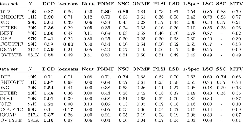
Table 4: Clustering performance using approximated KNN: (top) purities and (bottom) NMIs. Boldface numbers indicate the best in each row. “-” means out-of-memory error.
Data set N DCD k-means Ncut PNMF NSC ONMF PLSI LSD 1-Spec LSC SSC MTV
TDT2 10K 0.87 0.86 0.20 0.89 0.89 0.84 0.73 0.87 0.54 0.85 0.88 0.79 PENDIGITS 11K 0.90 0.71 0.12 0.70 0.63 0.61 0.36 0.58 0.43 0.78 0.83 0.77 20NG 20K 0.61 0.39 0.06 0.39 0.45 0.28 0.17 0.34 0.06 0.50 0.17 0.21 LETTER 20K 0.36 0.29 0.05 0.35 0.24 0.33 0.16 0.26 0.10 0.35 0.33 0.26 MNIST 70K 0.96 0.48 0.11 0.68 0.63 0.58 0.40 0.70 0.78 0.87 - 0.92 NORB 97K 0.41 0.22 0.30 0.25 0.30 0.25 0.30 0.38 0.30 0.20 - 0.30 ACOUSTIC 99K 0.59 0.60 0.50 0.54 0.50 0.54 0.50 0.52 0.55 0.57 - 0.53 MOCAP 217K 0.29 0.21 0.05 0.20 0.07 0.19 0.06 0.17 0.06 0.25 - 0.09 COVTYPE 581K 0.55 0.49 0.51 0.50 0.51 0.50 0.51 0.49 0.49 0.49 - 0.49
Data set N DCD k-means Ncut PNMF NSC ONMF PLSI LSD 1-Spec LSC SSC MTV
TDT2 10K 0.71 0.71 0.08 0.71 0.74 0.68 0.62 0.70 0.63 0.69 0.74 0.66 PENDIGITS 11K 0.87 0.68 0.00 0.69 0.57 0.61 0.25 0.58 0.55 0.76 0.77 0.78 20NG 20K 0.54 0.44 0.00 0.38 0.53 0.26 0.11 0.27 0.08 0.48 0.29 0.13 LETTER 20K 0.48 0.36 0.00 0.44 0.28 0.42 0.18 0.37 0.18 0.43 0.38 0.35 MNIST 70K 0.91 0.39 0.00 0.68 0.61 0.65 0.32 0.70 0.82 0.80 - 0.87 NORB 97K 0.22 0.00 0.13 0.05 0.13 0.05 0.09 0.18 0.16 0.00 - 0.10 ACOUSTIC 99K 0.14 0.17 0.00 0.05 0.03 0.06 0.04 0.07 0.15 0.14 - 0.09 MOCAP 217K 0.37 0.26 0.00 0.21 0.05 0.19 0.03 0.19 0.06 0.30 - 0.07 COVTYPE 581K 0.16 0.08 0.06 0.04 0.06 0.04 0.07 0.04 0.03 0.08 - 0.01 be obtained from any clustering methods, not necessarily center-based. Moreover, we use matrix divergences instead of only minimum or maximum of individual distances, which provides a more robust measure against outliers.
5.2 Input similarities
The inputs to DCD are the pairwise similarities between data items, for example the sym-metrized and binarized KNN graph used in Section 4. Naive implementation of KNN requiresO(N2) computational cost. There exist accelerated algorithms taking advantage of the fact that it is often not necessary to calculate all pairs but only those in local neighbor-hoods. We have used a simple implementation with a vantage-point index (Yianilos, 1993), where we slightly modified the code to admit sparse data and with interface to Matlab. For MNIST where N = 70,000, the accelerated KNN (with K = 10) algorithm requires in practice only about 7 minutes to completion..
Exact KNN by the above acceleration is still expensive for even larger data sets. In practice, we find that using highly accurate approximated KNN is enough for maintaining the DCD performance. Table 4 shows the comparison for large-scale data sets (N >10,000) using the Fast Library of Approximated Nearest Neighbors (FLANN; Muja and Lowe, 2014). We can see that the resulting DCD purities and NMIs are close to those with exact KNN, and that the accuracy gains over the other compared methods mostly remain. By using FLANN, we can obtain the similarities for DCD much faster; for example, FLANN takes about 30 seconds for MNISTwith K= 10.
which locally scales the spherical Gaussian kernels such that the neighborhoods around every data point have the same given entropy (Vladymyrov and Carreira-Perpi˜n´an, 2013), Sparse Manifold Clustering and Embedding that learns a sparse coding with respect to local manifold geometry and cluster distribution (Elhamifar and Vidal, 2011), andAnchorGraph which learns the low-rank sparse coding with a set of pre-clustered landmarks (Liu et al., 2010). Other approaches such as metric learning (e.g., Kulis, 2013) could also be applied to obtain better input similarities.
6. Conclusions
We have presented a new clustering method based on low-rank approximation with two major contributions: 1) a clusterability criterion which can be used for learning both clus-ter assignments and the number of clusclus-ters; 2) a relaxed formulation with novel low-rank doubly stochastic matrix decomposition which allows efficient optimization, as well as its multiplicative majorization-minimization algorithm. Experimental results showed that our method works robustly for various selected data sets and can substantially improve cluster-ing accuracy for large manifold data sets.
There are also some other generic characteristics which affect clustering performance. In the learning objective, there is the possibility of using other information divergences as the approximation error measure, including the matrix-wise and non-separable divergences (e.g., Cichocki et al., 2009; Dhillon and Tropp, 2007; Dikmen et al., 2015). In optimiza-tion, currently the multiplicative algorithm runs in batch mode. In the future we aim to develop even more scalable implementations such as streaming mini-batches of similarities and distributed computing. In this way DCD can be applicable to even bigger data sets and further improve clustering accuracy. In implementation, our practice indicates that initialization could play an important role because most current algorithms are only local optimizers. Using Dirichlet prior is only one way to smooth the objective function space. It is an open question whether other priors or regularization techniques could in general achieve better initializations.
Acknowledgments
This work was financially supported by the Academy of Finland (Finnish Centre of Excel-lence in Computational Inference Research COIN, grant no. 251170; Zhirong Yang addi-tionally by decision number 140398). We acknowledge the computational resources provided by the Aalto Science-IT project.
Appendix A. Proof of Theorem 1
Proof 1) Given a matrix B ∈ B and its corresponding W, let Uik = Wik/qPNv=1Wvk. Then B =U UT and
N X
j=1
Bij = N X
j=1 r X
k=1
WikWjk PN
v=1Wvk =
r X
k=1
WikPNj=1Wjk PN
v=1Wvk
=X k
That is, B ∈A. ThereforeB⊆A.
Appendix B. Proof of Theorem 2
Proof We useW and fW to distinguish the current estimate and the variable, respectively.
Let φijk =
are constants irrelevant to the variable Wf. The first two inequalities follow the CCCP majorization (Yang and Oja, 2011) using the convexity and concavity of−log() and log(), respectively. The third inequality is called “moving term” technique used in multiplicative updates (Yang and Oja, 2010). It adds the same constant a1
i +
α
Wik to both numerator and
(Minimization)
Setting the gradient to zero gives
Wiknew=Wik
Multiplying both numerator and denominator byai gives the last update rule in Algorithm 1. Therefore, L(Wnew, λ)≤G(Wnew, W)≤ L(W, λ).
References
M. Ackerman and S. Ben-David. Clusterability: A theoretical study. In Proceedings of the Twelfth International Conference on Artificial Intelligence and Statistics (AISTATS), pages 1–8, 2009.
D. Aloise, A. Deshpande, P. Hansen, and P. Popat. NP-hardness of euclidean sum-of-squares clustering. Machine Learning, 75(2):245–248, 2009.
R. Arora, M. Gupta, A. Kapila, and M. Fazel. Clustering by left-stochastic matrix fac-torization. In International Conference on Machine Learning (ICML), pages 761–768, 2011.
R. Arora, M. Gupta, A. Kapila, and M. Fazel. Similarity-based clustering by left-stochastic matrix factorization. Journal of Machine Learning Research, 14:1715–1746, 2013.
A. Asuncion, M. Welling, P. Smyth, and Y. Teh. On smoothing and inference for topic models. InConference on Uncertainty in Artificial Intelligence (UAI), pages 27–34, 2009.
M. Balcan, A. Blum, and S. Vempala. A discriminative framework for clustering via simi-larity functions. InACM symposium on Theory of Computing, pages 671–680, 2008.
M. Balcan, A. Blum, and A. Gupta. Approximate clustering without the approximation. In Proceedings of the Nineteenth Annual ACM-SIAM Symposium on Discrete Algorithms, pages 1068–1077, 2009.
S. Ben-David, N. Eiron, and H.U. Simon. The computational complexity of densest region detection. Journal of Computer and System Sciences, 64(1):22–47, 2002.
D. Blei, A. Ng, and M. Jordan. Latent dirichlet allocation. Journal of Machine Learning Research, 3:993–1022, 2001.
X. Bresson, T. Laurent, D. Uminsky, and J. von Brecht. Multiclass total variation clustering. In Advances in Neural Information Processing Systems (NIPS), pages 1421–1429, 2013.
D. Cai and X. Chen. Large scale spectral clustering via landmark-based sparse representa-tion. IEEE Transactions on Cybernetics, 45(8):1669–1680, 2015.
T. Calinski and J. Harabasz. A dendrite method for cluster analysis. Communications in Statistics, 3(1):1–27, 1974.
X. Chen and D. Cai. Large scale spectral clustering with landmark-based representation. In Conference on Artificial Intelligence (AAAI), 2011.
A. Cichocki, R. Zdunek, A. Phan, and S. Amari. Nonnegative Matrix and Tensor Factor-izations: Applications to Exploratory Multi-way Data Analysis. John Wiley, 2009.
D. Davies and D. Bouldin. A cluster separation measure. IEEE Transactions on Pattern Analysis and Machine Intelligence, 1(2):224–227, 1979.
I. Dhillon and J. Tropp. Matrix nearness problems with bregman divergences.SIAM Journal on Matrix Analysis and Applications, 29(4):1120–1146, 2007.
O. Dikmen, Z. Yang, and Erkki Oja. Learning the information divergence. IEEE Transac-tions on Pattern Analysis and Machine Intelligence, 37(7):1442–1454, 2015.
C. Ding, X. He, and H. Simon. On the equivalence of nonnegative matrix factorization and spectral clustering. InSIAM International Conference on Data Mining, 2005.
C. Ding, T. Li, W. Peng, and H. Park. Orthogonal nonnegative matrix t-factorizations for clustering. In International conference on Knowledge discovery and data mining (SIGKDD), pages 126–135, 2006.
C. Ding, T. Li, and M. Jordan. Nonnegative matrix factorization for combinatorial op-timization: Spectral clustering, graph matching, and clique finding. In International Conference on Data Mining (ICDM), pages 183–192, 2008.
C. Ding, T. Li, and M. Jordan. Convex and semi-nonnegative matrix factorizations. IEEE Transactions on Pattern Analysis and Machine Intelligence, 32(1):45–55, 2010.
E. Elhamifar and R. Vidal. Sparse subspace clustering. InConference on Computer Vision and Pattern Recognition (CVPR), 2009.
E. Elhamifar and R. Vidal. Sparse manifold clustering and embedding. In Advances in Neural Information Processing Systems (NIPS), pages 55–63, 2011.
S. Epter, M. Krishnamoorthy, and M. Zaki. Clusterability detection and initial seed se-lection in large data sets. Technical report, The International Conference on Knowledge Discovery in Databases, 1999.
C. F´evotte and J´erˆome Idier. Algorithms for nonnegative matrix factorization with the
β-divergence. Neural Computation, 23(9):2421–2456, 2011.
Z. He, S. Xie, R. Zdunek, G. Zhou, and A. Cichocki. Symmetric nonnegative matrix factorization: Algorithms and applications to probabilistic clustering.IEEE Transactions on Neural Networks, 22(12):2117–2131, 2011.
M. Hein and T. B¨uhler. An inverse power method for nonlinear eigenproblems with ap-plications in 1-spectral clustering and sparse pca. In Advances in Neural Information Processing Systems (NIPS), pages 847–855, 2010.
T. Hofmann. Probabilistic latent semantic indexing. In International Conference on Re-search and Development in Information Retrieval (SIGIR), pages 50–57, 1999.
B. Hopkins and J. Skellam. A new method for determining the type of distribution of plant individuals. Annals of Botany, 18(2):213–227, 1954.
D. Hunter and K. Lange. A tutorial on MM algorithms. The American Statistician, 58(1): 30–37, 2004.
B. Kulis. Metric learning: A survey. Foundations and Trends in Machine Learning, 5(4): 287–364, 2013.
D. Lee and H. Seung. Learning the parts of objects by non-negative matrix factorization. Nature, 401:788–791, 1999.
D. Lee and H. Seung. Algorithms for non-negative matrix factorization.Advances in Neural Information Processing Systems (NIPS), 13:556–562, 2001.
T. Liu and D. Tao. On the performance of manhattan nonnegative matrix factorization. IEEE Transactions on Neural Networks and Learning Systems, 27(9):1851–1863, 2016.
W. Liu, J. He, and S. Chang. Large graph construction for scalable semi-supervised learning. In International Conference on Machine Learning (ICML), pages 679–686, 2010.
S. Lloyd. Least square quntization in pcm. IEEE Transactions on Information Theory, 28 (2):129–137, 1982.
M. Mahajan, P. Nimbhorkar, and K. Varadarajan. The planar k-means problem is np-hard. In Lecture Notes in Computer Science, volume 5431, pages 274–285. Springer, 2009.
T. Minka. Estimating a Dirichlet distribution, 2000.
A. Ng, M. Jordan, and Y. Weiss. On spectral clustering: Analysis and an algorithm. In Advances in Neural Information Processing Systems (NIPS), pages 849–856, 2001.
R. Ostrovsky, Y. Rabani, L. Schulman, and C. Swamy. The effectiveness of lloyd-type methods for the k-means problem. In Proceedings of the 47th Annual IEEE Symposium on Foundations of Computer Science, pages 165–176, 2006.
F. Pompili, N. Gillis, P. Absil, and F. Glineur. ONP-MF: An orthogonal nonnegative matrix factorization algorithm with application to clustering. In European Symposium on Artificial Neural Networks,, pages 297–302, 2013.
A. Rodriguez and A. Laio. Clustering by fast search and find of density peaks. Science, 344 (6191):1492–1496, 2014.
J. Shi and J. Malik. Normalized cuts and image segmentation. IEEE Transactions on Pattern Analysis and Machine Intelligence, 22(8):888–905, 2000.
R. Sinkhorn and P. Knopp. Conerning non-negative matrices and doubly stochastic matri-ces. Pacific Journal of Mathematics, 21:343–348, 1967.
J. Sinkkonen, J. Aukia, and S. Kaski. Component models for large networks. ArXiv e-prints, 2008.
N. Srivastava, R. Salakhutdinov, and G. Hinton. Modeling documents with deep Boltzmann machines. In Proceedings of the Twenty-Ninth Conference on Uncertainty in Artificial Intelligence, (UAI), 2013.
R. Tibshirani, G. Walther, and T. Hastie. Estimating the number of clusters in a data set via the gap statistic. Journal of the Royal Statistical Society: Series B, 63, Part 2: 411–423, 2001.
N. Vinh, J. Epps, and J. Bailey. Information theoretic measures for clusterings compari-son: variants, properties, normalization and correction for chance. Journal of Machine Learning and Research, 11:2837–2854, 2010.
M. Vladymyrov and M. Carreira-Perpi˜n´an. Entropic affinities: properties and efficient numerical computation. InInternational Conference on Machine Learnin (ICML), pages 477–485, 2013.
F. Wang, P. Li, A. K¨onig, and M. Wan. Improving clustering by learning a bi-stochastic data similarity matrix. Knowledge Information Systems, 32(2):351–382, 2012.
Z. Yang and J. Laaksonen. Multiplicative updates for non-negative projections. Neurocom-puting, 71(1-3):363–373, 2007.
Z. Yang and E. Oja. Linear and nonlinear projective nonnegative matrix factorization. IEEE Transaction on Neural Networks, 21(5):734–749, 2010.
Z. Yang and E. Oja. Clustering by low-rank doubly stochastic matrix decomposition. In International Conference on Machine Learning (ICML), pages 831–838, 2012a.
Z. Yang and E. Oja. Quadratic nonnegative matrix factorization. Pattern Recognition, 45 (4):1500–1510, 2012b.
Z. Yang, Z. Yuan, and J. Laaksonen. Projective non-negative matrix factorization with applications to facial image processing. International Journal on Pattern Recognition and Artificial Intelligence, 21(8):1353–1362, 2007.
P. Yianilos. Data structures and algorithms for nearest neighbor search in general met-ric spaces. In Proceedings of the Fourth Annual ACM-SIAM Symposium on Discrete Algorithms (SODA), pages 311–321, 1993. We have modified and used the code in
http://stevehanov.ca/blog/index.php?id=130.
J. Yoo and S. Choi. Orthogonal nonnegative matrix factorization: Multiplicative updates on Stiefel manifolds. InIntelligent Data Engineering and Automated Learning (IDEAL), pages 140–147, 2008.
S. Yu and J. Shi. Multiclass spectral clustering. In IEEE International Conference on Computer Vision (ICCV), pages 313–319, 2003.
R. Zass and A. Shashua. Doubly Stochastic Normalization for Spectral Clustering. In Advances in Neural Information Processing Systems (NIPS), 2006.