User Model User-Adap Inter DOI 10.1007/s11257-007-9046-5
O R I G I NA L PA P E R
A multifactor approach to student model evaluation
Michael V. Yudelson · Olga P. Medvedeva · Rebecca S. Crowley
Received: 11 December 2006 / Accepted in revised form: 20 December 2007 © Springer Science+Business Media B.V. 2008
Abstract Creating student models for Intelligent Tutoring Systems (ITS) in novel domains is often a difficult task. In this study, we outline a multifactor approach to evaluating models that we developed in order to select an appropriate student model for our medical ITS. The combination of areas under the receiver-operator and precision-recall curves, with residual analysis, proved to be a useful and valid method for model selection. We improved on Bayesian Knowledge Tracing with models that treat help differently from mistakes, model all attempts, differentiate skill classes, and model forgetting. We discuss both the methodology we used and the insights we derived regarding student modeling in this novel domain.
M. V. Yudelson·O. P. Medvedeva·R. S. Crowley
Department of Biomedical Informatics, University of Pittsburgh School of Medicine, Pittsburgh, PA, USA
M. V. Yudelson e-mail: [email protected] O. P. Medvedeva
e-mail: [email protected] M. V. Yudelson
School of Information Sciences, University of Pittsburgh, Pittsburgh, PA, USA R. S. Crowley
Intelligent Systems Program, University of Pittsburgh, Pittsburgh, PA, USA R. S. Crowley
Department of Pathology, University of Pittsburgh School of Medicine, Pittsburgh, PA, USA R. S. Crowley (
B
)Keywords Student modeling·Intelligent tutoring systems·Knowledge Tracing·
Methodology·Decision theory·Model evaluation·Model selection·Intelligent medical training systems ·Machine learning ·Probabilistic models· Bayesian models·Hidden Markov Models
1 Introduction
Modeling student knowledge in any instructional domain typically involves both a high degree of uncertainty and the need to represent changing student knowledge over time. Simple Hidden Markov Models (HMM) as well as more complex Dynamic Bayes-ian Networks (DBN) are common approaches to these dual requirements that have been used in many educational systems that rely on student models. One of the first quantitative models of memory (Atkinson and Shiffrin 1968) introduced the proba-bilistic approach in knowledge transfer from short to long term memory. Bayesian Knowledge Tracing (BKT) is a common method for student modeling in Intelli-gent Tutoring Systems (ITS) which is derived from the Atkinson and Shiffrin model (Corbett and Anderson 1995). BKT has been used successfully for over two decades in cognitive tutors for teaching computer science and math. One of the main advantages of the BKT approach is its simplicity. Within the specific domains where BKT is used, this method has been shown to be quite predictive of student performance (Corbett and Anderson 1995).
More complex DBN models of student performance have been developed for ITS, but are infrequently used. For the Andes physics tutor, Conati et al. developed a DBN that modeled plan recognition and student skills (Conati et al. 2002). It supported prediction of student actions during problem solving and modeled the impact ofhint requeston student skill transition from the unmastered to mastered state. The Andes BN modeled skills as separate nodes and represented dependencies between them. Because of the large size of the resulting network, parameters were estimates based on expert belief. Recently, other researchers presented a machine learning approach to acquiring the parameters of a DBN that modeled skill mastery based on three possible outcomes of user actions:correct,incorrect andhint request(Jonsson et al. 2005). This model was trained on simulated data.
A multifactor approach to student model evaluation
formalism based on a set of permutations of key model variables. Finally, we show that the resulting selected models perform well on external testing data unrelated to the original tutoring system.
2 Background
2.1 Classical knowledge tracing
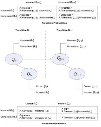
Bayesian Knowledge Tracing (BKT) is an established method for student modeling in intelligent tutoring systems, and therefore constituted our baseline model. BKT rep-resents the simplest type of Dynamic Bayesian Network (DBN)—a Hidden Markov Model (HMM), with one hidden variable (Q) and one observable variable (O) per time slice (Reye 2004). Each skill is modeled separately, assuming conditional inde-pendence of all skills. Skills are typically delineated using cognitive task analysis, which guides researchers to model skill sets such that an assumption of conditional independence of skills is valid (Anderson 1993). As shown in Fig.1, the hidden var-iable has two states, labeledmasteredandunmastered, corresponding to thelearned
andunlearnedstates described by Corbett et al. (Corbett and Anderson 1995). The observable variable has two values, labeledcorrectandincorrect, corresponding to the
correctandincorrectobservables described by Corbett et al. (Corbett and Anderson 1995). Throughout this paper, we refer to this topology as the BKT topology.
The transition probabilities describe the probability that a skill is (1) learned (tran-sition from unmastered state to mastered state), (2) retained (tran(tran-sition from mastered state to mastered state), (3) unlearned (transition from unmastered state to unmas-tered state), and (4) forgotten (transition from masunmas-tered state to unmasunmas-tered state). In all previously described implementations, BKT makes the assumption that there is no forgetting and thereforePretained is set to 1 andPforgotten is set to 0. With this
assumption, the conditional probability matrix can be expressed using the single prob-abilityPlearned, corresponding to the ‘transition probability’ described by Corbett et al.
(Corbett and Anderson 1995).
The emission table describes the probability of the response conditioned on the internal state of the student. As described by Corbett et al., the slip probability (Pslip) represents the probability of an incorrect answer given that the skill is in the known state, and the guess probability (Pguess) represents the probability of a correct answer
given that the skill is in the unknown state. Probabilities for the other two emissions are not semantically labeled. Throughout this paper, we refer to the implementation of BKT described by Corbett and Anderson in their original paper (Corbett and Anderson 1995) as “classical BKT”.
2.2 Key assumptions of classical Bayesian Knowledge Tracing
Fig. 1 Hidden Markov Model representing a general formalism for Bayesian Knowledge Tracing
mastered to unmastered state; and (3) model parameters are typically estimated by experts. A detailed explanation of each assumption and its potential disadvantages is provided below.
2.3 Multiple-state hidden and observed variables
A multifactor approach to student model evaluation
typically detect at least one more type of action—hint or request for help. In classical BKT, hints are considered as incorrect actions (Corbett and Anderson 1995), since the skill mastery is based on whether the user was able to complete the step without hints and errors. In other implementations of BKT, modeling of hint effect is considered to have a separate influence, by creating a separate hidden variable for hints which may influence the hidden variable for student knowledge (Jonsson et al. 2005), the observable variable for student performance, (Conati and Zhao 2004), or both of these variables (Chang et al. 2006).
The BKT topology also makes the assumption of a binary hidden node, which models the state of skill acquisition asknownormasteredversusunknownor unmas-tered. This is a good assumption when cognitive models are based on unequivo-cally atomic skills in well-defined domains. Examples of these kinds of well-defined domains include Algebra and Physics. Many ill-defined domains like medicine are dif-ficult to model in this way because skills are very contextual. For example, identifying a blister might depend on complex factors like the size of the blister which are not accounted for in our cognitive model. It is impractical in medicine to conceptualize a truly atomic set of conditionally independent skills in the cognitive model that accounts for all aspects of skill performance. Thus, development of a cognitive model and student model in medical ITS presupposes that we will aggregate skills together. Some researchers have already begun to relax these constraints. For example, Beck and colleagues have extended the BKT topology by introducing an intermediate hid-den binary node to handle noisy stuhid-dent data in tutoring systems for reading (Beck and Sison 2004). Similarly, the BN in the constraint-based CAPIT tutoring system (Mayo and Mitrovic 2001) used multiple state observable variables to predict the outcome of the next attempt for each constraint. However, the CAPIT BN did not explicitly model unobserved student knowledge.
From an analytic viewpoint, the number of hidden states that are supported by a data set should not be fewer than the number of observed actions (Kuenzer et al. 2001), further supporting the use of a three-state hidden node for mastery, when hint request is included as a third observable state. Although researchers in domains outside of user modeling have identified that multiple hidden-state models are more predictive of performance (Seidemann et al. 1996), to our knowledge there have been no previous attempts to test this basic assumption in ITS student models.
2.4 Modeling forgetting
populations, but not for individuals. This approach has the advantage of providing a method for modeling forgetting over long time intervals based on a widely-accepted psychological construct. However, the poor performance for predicting individual stu-dent learning could be problematic for ITS stustu-dent models. Another disadvantage of this approach is that it cannot be easily integrated with formalisms that provide prob-abilistic predictions based on multiple variables, in addition to time. It may be that including the kind of memory decay suggested by Jastrzembski and colleagues into a Bayesian formalism could enhance the prediction accuracy for individuals. In one of our models, we attempt to learn the memory decay directly from individual students’ data.
2.5 Machine learning of DBN
Classical BKT is typically used in domains where there has been significant empirical task analytic research (Anderson et al. 1995). These domains are usually well-struc-tured domains, where methods of cognitive task analysis have been used successfully over many years to study diverse aspects of problem-solving. Researchers in these domains can use existing data to create reliable estimates of parameters for their models. In contrast, novel domains typically lack sufficient empirical task analytic research to yield reasonable estimates. In these domains, machine learning provides an attractive, alternative approach.
Although some researchers have used machine learning techniques to estimate probabilities for static student modeling systems (Ferguson et al. 2006), there have been few attempts to learn probabilities directly from data for more complex dynamic Bayesian models of student performance. Jonsson and colleagues learned probabilities for a DBN to model student performance, but only with simulated data (Jonsson et al. 2005). Chang and colleagues have also used machine learning techniques. They note that forgetting can be modeled with the transition probability using the BKT topology; however, the authors set the value ofPforgottento zero which models the no-forgetting
assumption used in classical BKT (Chang et al. 2006).
2.6 Model performance metrics
Student model performance is usually measured in terms of actual and expected accu-racies, where actual accuracy is the number of correct responses averaged across all users and expected accuracy is a model’s probability of a correct response averaged across all users. For example, Corbett and Anderson used correlation, mean error and mean absolute error to quantify model validity (Corbett and Anderson 1995). A disad-vantage of this approach is that it directly compares the categorical user answer (correct
A multifactor approach to student model evaluation
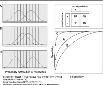
Fig. 2 ROC Curve and related performance metrics definitions
errors. Instead, Receiver-Operating Characteristic (ROC) curves have been advocated because they make these tradeoffs explicit (Provost et al. 1998). Additionally, accuracy alone can be misleading without some measure of precision.
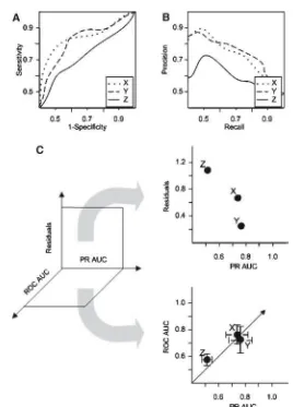
Recently, the Receiver-Operating Characteristic curve (ROC), which is a trade-off between the true positive and false negative rates (Fig.2), has been used to evaluate student models (Fogarty et al. 2005;Chang et al. 2006). Figure2(left) shows three models in terms of their ability to accurately predict user responses. Models that have more overlap between predicted and actual outcome have fewer false positives and false negatives. For each model, a threshold can be assigned (vertical lines) that pro-duces a specific combination of false negatives and false positives. These values can then be plotted as sensitivity against 1-specificity to create the ROC curve. Models with larger areas under the curve have fewer errors than those with smaller areas under the curve.
sensitivity-specificity trade-off. However, no prior research has directly tested the validity and feasibility of such methods for student model selection. Figure2(bottom) defines commonly used machine learning evaluation metrics based on the contingency matrix. These metrics cover all possible dimensions:Sensitivityor Recalldescribes how well the model predicts the correct results, Specificitymeasures how well the model classifies the negative results, and Precision measures how well the model classifies the positive results.
2.7 Summary of present study in relationship to previous research
In summary, researchers in ITS student modeling are exploring a variety of adapta-tions to classical BKT including alteraadapta-tions to key assumpadapta-tions regarding observable and hidden variables states, forgetting, and use of empirical estimates. In many cases, these adaptations will alter the distribution of classification errors associated with the model’s performance. This paper proposes a methodology for student model com-parison and selection that enables researchers to investigate and differentially weigh classification errors during the selection process.
2.8 Research objectives
Development of student models in complex cognitive domains such as medicine is impeded by the absence of task analytic research. Key assumptions of commonly used student modeling formalisms may not be valid. We required a method to test many models with regard to these assumptions and select models with enhanced per-formance, based on tradeoffs among sensitivity, specificity and precision (predictive value).
Therefore, objectives of this research project were to:
(1) Devise a method for evaluating and selecting student models based on decision theoretic evaluation metrics
(2) Evaluate the model selection methodology against independent student perfor-mance data
(3) Investigate effect of key variables on model performance in a medical diagnostic task
3 Cognitive task and existing Tutoring system
A multifactor approach to student model evaluation
Clancey 1984). In medicine, visual classification problem solving is an important aspect of expert performance in pathology, dermatology and radiology.
Cognitive task analysis shows that practitioners master a variety of cognitive skills as they acquire expertise (Crowley et al. 2003). Five specific types of subgoals can be identified: (1) search and detection, (2) feature identification, (3) feature refine-ment, (4) hypothesis triggering and (5) hypothesis evaluation. Each of these subgoals includes many specific skills. The resulting empirical cognitive model was embedded in the SlideTutor system. Like other model tracing cognitive ITS, SlideTutor deter-mines both correct and incorrect student actions as well as the category of error that has been made and provides an individualized instructional response to errors and hint requests. The student model for SlideTutor will be used by the pedagogic system to select appropriate cases based on student mastery of skills and to determine appropri-ate instructional responses by correlating student responses with learning curves, so that the system can encourage behaviors that are associated with increased learning and discourage behaviors that are associated with decreased learning.
In this paper, we analyzed student models created for two specific subgoals types:
Feature-IdentificationandHypothesis-Triggering. We selected these subgoals because our previous research showed that correctly attaching symbolic meaning to visual cues and triggering hypothesis are among the most difficult aspects of this task (Crowley et al. 2003).
4 Methods
4.1 Student model topologies
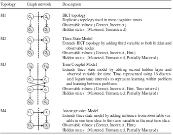
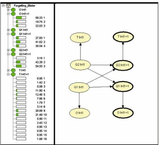
We evaluated 17 different model topologies for predicting the observed outcome of user action. For simplicity, only four of these are shown in Table 1. Network graphs represent two subsequent time slices for the spatial structure of each DBN, separated by a dotted line. Hidden nodes are shown as clear circles. Observed nodes are shown as shaded circles. Node subscript indicates number of node states (for hidden nodes) or values (for observable nodes).
Topology M1 replicates the BKT topology (Corbett and Anderson 1995), as described in detail in the background section of this paper (Fig.1) but does not set thePforgottentransition probability to zero. In this model, hint requests are counted as
incorrect answers.
Topology M2 extends the BKT topology in M1 by adding a third state for the hid-den variable—partially mastered; and a third value for the observable variable—hint. This creates emission and transition conditional probability matrices with a total of nine probabilities respectively, as opposed to the four emission probabilities possible using the BKT topology. In the case of classical BKT, this is simplified to two probabilities for the transition matrix by the no forgetting assumption.
Table 1 Dynamic Bayesian Network (DBN) Topologies
Replicates topology used in most cognitive tutors Observable values: {Correct, Incorrect}
Extends BKT topology by adding third variable to both hidden and observable nodes.
Observable values: {Correct, Incorrect, Hint}
Hidden states: {Mastered, Unmastered, Partially Mastered} M3
Extends three state model by adding second hidden layer and observed variable for time. Time represented using 16 discret-ized logarithmic intervals to represent learning within problem and learning between problems.
Observable values: {Correct, Incorrect, Hint, Time interval} Hidden states: {Mastered, Unmastered, Partially Mastered}
M4 Q3
O3 O3
Q3 Autoregressive Model
Extends three state model by adding influence from observable var-iable in one time slice to the same varvar-iable in the next time slice. Observable values: {Correct, Incorrect, Hint}
Hidden states: {Mastered, Unmastered, Partially Mastered}
time variable includes 16 discretized logarithmic time intervals. We used a time range of 18 h—the first 7–8 intervals represents the user’s attempts at a skill between skill opportunities in thesame problemand the remaining time intervals represent the user’s attempts at a skill between skill opportunities indifferent problems.
Topology M4 (Ephraim and Roberts 2005) extends the three state model in M2 by adding a direct influence of the observable value in one time slice to the same vari-able in the next time slice. Therefore this model may represent a separate influence of student action upon subsequent student action, unrelated to the knowledge state. For example, this topology could be used to model overgeneralization (e.g. re-use of a diagnostic category) or automaticity (e.g. repeated use of the hint button with fatigue). All model topologies share two assumptions. First, values in one time slice are only dependent on the immediately preceding time-slice (Markov assumption). Second, all skills are considered to be conditionally independent. None of the models make an explicit assumption of no forgetting, and thusPunlearnedis learned directly from the
data.
4.2 Tools
A multifactor approach to student model evaluation
Bayes Net Toolbox (BNT) for Matlab (Murphy 2001). Other researchers have also extended BNT for use in cognitive ITS (Chang et al. 2006). Among other features, BNT supports static and dynamic BNs, different inference algorithms and several methods for parameter learning. The only limitation we found was the lack of BN visualization for which we used the Hugin software package with our own application programming interface between BNT and Hugin. We also extended Hugin to implement an infinite DBN using a two time-slice representation. The Matlab–Hugin interface and Hugin 2-time-slices DBN extension for infinite data sequence were written in Java.
4.3 Experimental data
We used an existing data set derived from 21 pathology residents (Crowley et al. 2007). The tutored problem sequence was designed as an infinite loop of 20 problems. Stu-dents who completed the entire set of 20 problems restarted the loop until the entire time period elapsed. The mean number of problems solved was 24. The lowest number of problems solved was 16, and the highest number of problems solved was 32. The 20-problem sequence partially covers one of eleven of SlideTutor’s disease areas. The sequence contains 19 of 33 diseases that are supported by 15 of 24 visual features of the selected area.
User-tutor interactions were collected and stored in an Oracle database. Several levels of time-stamped interaction events were stored in separate tables (Medvedeva et al. 2005). For the current work, we analyzed client events that represented student
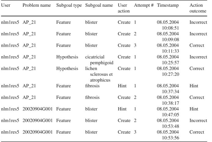
Table 2 Example of student record sorted by timestamp
User Problem name Subgoal type Subgoal name User Attempt # Timestamp Action
action outcome
nlm1res5 AP_21 Feature blister Create 1 08.05.2004 10:08:51
Incorrect nlm1res5 AP_21 Feature blister Create 2 08.05.2004
10:09:08
Incorrect nlm1res5 AP_21 Feature blister Create 3 08.05.2004
10:11:33
nlm1res5 AP_21 Feature fibrosis Hint 1 08.05.2004 10:37:34
Hint nlm1res5 AP_21 Feature fibrosis Create 2 08.05.2004
10:38:17
Correct nlm1res5 20020904G001 Feature blister Hint 1 08.05.2004
10:47:05 Hint nlm1res5 20020904G001 Feature blister Create 2 08.05.2004
10:53:48
Incorrect nlm1res5 20020904G001 Feature blister Create 3 08.05.2004
10:53:56
behaviors in learning feature identification and hypothesis triggering, including three outcomes:Correct,IncorrectorHintrequest (Table2).
During the study, all students received the same pre-test, post-test and retention test. All tests were computer-based and had identical structure, including case diagnosis and multiple-choice sections. In theCase Diagnosis Section,students had to apply all required cognitive skills to make a diagnosis or differential diagnosis for a particular case. In contrast, theMultiple-Choice Sectioncontained 51 multiple-choice questions to test student knowledge on different subgoals, including feature identification ques-tions (post-testN =12; retention-testN =17) and hypothesis triggering questions (post-testN =21; retention-testN=23).
4.4 Data partitioning and aggregation
Data partitions represent an additional dimension for selecting appropriate student models. As part of our investigations, we explored the effect of different methods of data partitioning on model performance for models that exceeded baseline per-formance. The combined data from user actions and action outcomes from tutored sessions were extracted from student records in our student protocol database into a data hypercube (Table2) with the following dimensions: user name, problem name, subgoal type (Feature, Hypothesis), subgoal name, user action (Create, Hint), enumer-ated attempts to identify each subgoal within the problem, timestamp, and user action outcome (Correct, Incorrect, Hint). Since our tutoring system provided immediate feedback, we excluded the user action “Delete subgoal x” from student modeling.
The data were partitioned or aggregated along three dimensions, as shown in Table3. First, we partitioned data by the number of user attempts to complete the subgoal within the problem, considering (1)first attemptonly or (2)all attempts. Sec-ond, we partitioned data by subgoal class creating three groups: (1) data related to learning of feature-identification, (2) data related to learning of hypothesis-triggering, or (3) all data related to learning of either class. Third, we partitioned data by subgoal instance considering: (1)eachsubgoal separately, or (2) all subgoals together. The total number of datapoints refers to the user action outcomes used as input for the models.
4.5 Procedure for learning model parameters
Models were learned for each topology across every data partition. Inputs to the models consisted of observed values and time node calculations from the data hypercube. Fol-lowing completion of model training, each model-partition combination was evaluated against student test data.
4.5.1 Observed values for models
All 4 model topologies use ACTION OUTCOME as an observed value (Table 2,
A
m
ultif
actor
approach
to
student
model
ev
aluation
Table 3 Comparison of data partitions and models tested
Number of 1st attempt All attempts
attempts
Subgoal class Feature Hypothesis All data (F, H) Feature Hypothesis All data (F, H)
Subgoal instance Each All Each All All Each All Each All All
Model topologies M1 M2 M3 M1 M2 M3 M1 M2 M3 M1 M2 M3 M1 M2 M3 M1 M2 M3 M1 M2 M3 M1 M2 M3 M1 M2 M3 M1 M2 M3 M4
Model number 4 14 23 1 11 21 5 15 24 2 12 22 3 13 29 9 19 27 6 16 25 10 20 28 7 17 26 8 18 30 31 Number of
datapoints
2,363 1,621 3,984 4,054 2,233 6,287
uses the TIMESTAMP as a time node T16 (Table1) observed value. The time node
inputt_valuerepresents a discretized time interval between the attempts. Due to the asynchronous nature of the time coupled HMM, wheret_valuein the current state will influence an answer in the next time slice,t_valuewas calculated using the formula:
t_valuet =ceil(log2(Timestampt+1−Timestampt))
For example, for the last attempt to identify blister in case AP_21 (Table2, row 3),
t_value=12, based on Timestampt+1=08.05.2004 10:47:05 (Table2, row 8) and
Timestampt =08.05.2004 10:11:33 (Table2, row 3). In this particular example, the time interval reflects skill performance changes across two different cases.
4.5.2 Time series inputs to the models
Inputs to the models consisted of time series extracted from the hypercube. Let us consider each possible action outcome value to be represented by (1=Correct, 2=Incorrect, 3=Hint). Based on the data sample in Table 2, the time series for model topology=M1, for (Subgoal Class=Feature, Subgoal Instance=blister, All Attempts) can be represented by the six Blister events as follows:
[2] [2] [1] [2] [2] [1]
where entries in square bracket represent the values for action outcome, because in topology=M1 we consider hints to be incorrect actions. Using the same data partition, the data for model topology=M2 or topology=M4 can be represented as:
[2] [2] [1] [3] [2] [1]
because in topologies M3 and M4 we consider hint as a separate action. Topology=M4 introduces a second dimension time observable into each event in the series based on the interval between the current event and next event (see Sect.4.5.1),
[2, 5] [2, 8] [1, 12] [3, 9] [2, 3] [1, 16]
As shown in the preceding section, the third attempt at blister results in a correct outcome with a computedt_value=12.
4.5.3 Model training and testing
The model parameters were learned using the classic Expectation-Maximization algo-rithm for DBN (Murphy 2001) with 10 iterations or until the logaalgo-rithmic likelihood increased less than one per million (0.001). Prior probabilities and conditional prob-abilities were initialized using random values. Model testing was performed using k-fold cross-validation method withk = 5. The tutored dataset was divided into 5 subsets: 4 subsets contain 4 students each and the 5th subset—5 students. We sequen-tially advanced through the subsets, using 4 subsets for training and 1 for testing the model. Each data point, a value of observed variable was used once for testing and 4 times for training.
A multifactor approach to student model evaluation
Fig. 3 Example of DBN visualization: model M3 for feature blister (two times slices)
were visualized using Hugin. Figure3shows an example of a learned model M3 for Feature=blister. The left panel shows the probabilities for all hidden and observable nodes in the second time slice.
4.5.4 Model validation
Models trained for Subgoal Class=All Data were tested for the two Subgoal Classes (feature identification and hypothesis-triggering) separately. Models learned only on tutored data were then evaluated against post-test and retention test data as an external validation set.
4.6 Performance metrics
We compared performance of the resulting models using 3 evaluation metrics:
To compare models, a two-dimensional ROC can be reduced to a single scalar value representing expected performance (Fawcett 2003). The area under the ROC curve (ROC AUC) is equivalent to a probability of how well the model dis-tinguishes between two classes. In a statistical sense, ROC AUC shows the size of the “overlap” of the classification distributions. An ROC AUC of 0.5 represents a random classifier. The ideal model will have an ROC AUC of 1. ROC metrics is dataset independent—models built on the datasets with different distribution of positive (or negative) outcomes can be directly compared to each other. The ROC AUC is equivalent to the Wilcoxon statistic (Hanley and McNeil 1982). To determine which models should be considered for further study, we can use the pairwise model comparison method described by Hanley and McNeil to test if a model is more predictive than chance. In this case, the second model in the
Ztest should have ROC AUC=0.5 and standard error=0 (Fogarty et al. 2005). Significance of the Z test outcome is determined using a standard table. For
z-value≥2.326, P≤.01.
(2) Precision-Recall Curve (PR)is used to express the trade-off between complete-ness (Recall) and usefulcomplete-ness (Precision) of the model. The PR curve can be obtained with the same threshold technique that was used for ROC curves. In anology to ROC AUC, we can define the area under a PR curve as the PR AUC (Davis and Goadrich 2006). The area under the PR hyperbolic curve for an ideal model is equal to 1. Precision (Positive Predictive Value) (Fig.2) depends on the frequency of positive outcomes in the dataset. Therefore, the PR metrics is dataset dependent.
(3) Residual—is a quantitative measure of goodness of fit. Residual is defined as the difference between actual (observed) and estimated (predicted) value for numeri-cal outcome (Moore and McCabe 2003). The residuals metric is used to measure model performance as a whole rather than focusing on what the data implies about any given model’s individual outcome. Residuals are generally inspected using a visual representation. The residual plot shows residuals as a function of the measured values. A random pattern around 0-value of residuals indicates a good fit for a model. For an integrated measure of residuals for each model, we calculated the norm of residual (NR) for each user using the following formula:
NR=√(Fa−Fe)2
where the summation is performed over all the subgoals, Fais the actual success
rate−the number of correct answers averaged by subgoal for each user, and Fe
is an estimated success−the number of predicted correct answers averaged by subgoal for each user. NR averaged across all users represents a quantitative metric for each model. Better models have smaller residuals.
consider-A multifactor approach to student model evaluation
Fig. 4 Performance metrics. (a) ROC curves, (b) PR curves, (c) 3-D performance metrics
ation. Models X and Y have no significant differences in PR-ROC AUC space. These models can be separated using the residual metric (Fig.4c, top right). Model Y has the smallest residual, so it can be considered to be the best model for a given data set. To use the binary ROC metric for model comparison, we limit our analysis to cor-rect vs. other possible outcomes, since the final goal is to predict the corcor-rect answers on post-test or retention test.
4.7 Statistical analysis
of factor differences, we first applied the Lilliefors test to evaluate the normality of each parameter distribution and determined that the assumption of normality was not met. Consequently, we used the Kruskal–Wallis test—a nonparametric version of the classical one-way ANOVA that extends the Wilcoxon rank sum test for multiple mod-els. The Kruskal–Wallis test uses the Chi-square statistic with (number of groups-1) degrees of freedom to approximate the significance level, and returns a P-value for the null hypothesis that all models are drawn from a population with the same median. If aP-value is close to 0, then the null hypothesis can be rejected, because at least one model median is significantly different from the other ones.
To analyze the performance of the models as individuals, we performed the Krus-kal-Wallis test for all 3 evaluation metrics parameters without factoring the data to determine that at least one model for each metric is significantly different from the others. We then performed the follow-up Tukey–Kramer test for pairwise comparisons of the average ranks of models. In Matlab, the Tukey–Kramer test function provides a graphical output which was used to visualize the difference between models. Each model in this graph is represented by a point with surrounding 95% confidence inter-val. Two models are significantly different if their intervals are disjoint and are not significantly different if their intervals overlap.
5 Results
We applied multi-dimensional performance analysis to select the best models trained on the tutored data set. Models selected using this procedure were then validated on post-test and retention test data.
5.1 Model assessment procedures
A result of this work is that we refined a process for step-wise model selection using three performance metrics (ROC, PR and Residuals) to select the best model. The resulting process is general and can be applied to other ITS student modeling. In particular, this method may be useful in assessing potential student models in novel domains where assumptions of existing student model formalisms for other domains may not be valid.
Our general approach was to carry out model evaluation in two steps:
(1) Preliminary model selectionROC and PR curves, and AUC metrics were used as an initial rapid screening method to eliminate models with performance inferior to the baseline.
(2) Model performance comparison For each remaining model, we then computed three performance metrics (ROC AUC, PR AUC, and Residuals) and compared them using variables such as model topology or subgoal grouping as factor levels.
A multifactor approach to student model evaluation
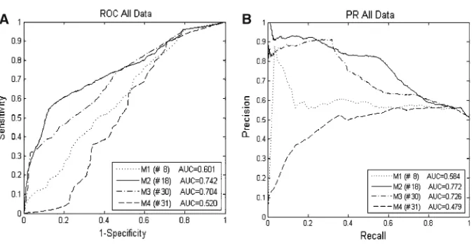
Fig. 5 Rejection of topology M4 during step one of model evaluation
5.2 Step one—preliminary model selection by ROC analysis
During preliminary model topology selection, we rejected the models with the lowest AUC in both ROC and PR spaces. A total of seventeen (17) model topologies were evaluated during this step, from which we rejected fourteen (14) models, leaving 3 topologies for further consideration. Figure5shows an example of the model rejection process.
The figure depicts ROC curves (5A) and PR curves (5B) for model topologies M1, M2, M3 and M4 for the same dataset which consists of Subgoal Class=All Data with Number of Attempts=All (Table3). Model topology M4 (Fig.5, dashed line) can be rejected, because it does not dominate in any area of the ROC or PR space, and the AUC in both spaces is lower than the AUC of our baseline BKT model M1. M4 is representative of all fourteen models that were rejected during this step.
Z-test shows that Model #31 is not significantly better than chance (P > .21) and can therefore be excluded from further consideration (Table4).
5.3 Step two—model performance analysis
In the second step, we compared remaining models using the three evaluation metrics for each partitioning variable in succession.
Table 4 Z-test results for ROC
AUC for models in Fig.5 Model Z-value P
8 2.368 < .01
18 6.411 < .001
30 8.487 < .001
5.3.1 Model evaluation
We evaluated models trained on different data partitions with respect to different fac-tors: (1) Model Topology, (2) Subgoal instance Grouping, and (3) Number of Attempts. For each of the models trained on a particular dataset, we obtained three performance metrics: (1) ROC AUC, (2) PR AUC, and (3) Residuals. These measures were used to determine the optimal combination of topology and partitioning factors. Analysis was separately performed for feature identification and hypothesis-triggering because we cannot directly compare data from these two separate skills. Additionally, we had a stronga prioriassumption that feature identification and hypothesis triggering might be represented best by different models and, therefore, preferred to examine the models separately.
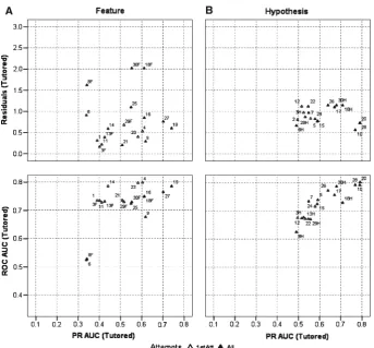
Figures6–8show a comprehensive view of the computed metrics for models based on tutored data only. Models are shown in three-dimensional ROC-PR-Residuals space. Each model is labeled with its corresponding model number from Table 3. For models that used All data for features and hypotheses (models 3, 13, 29, 8, 18, and 30), we trained the models on all data, but computed separate metrics for testing against feature data or testing against hypothesis data. These models are presented using superscripts (F and H) in all figures. Figure6shows model performance sep-arating models by 1st attempt (open triangles) versus all attempts (closed triangles) partitioning factor. Figure 7 shows model performance separating models by each instance (closed squares) versus all instances (open squares) partitioning factor. Fig-ure8shows model performance separating models by topology, where M2 models are represented by open circles, M3 models are represented by closed circles, and M1 models are represented by crosses.
Using this method, we can determine the relative benefit of a particular factor selection across all models.
From Figure6, it is clear that models using all attempts (closed circles) generally perform better than models using only 1st attempts (open circles). These models have higher PR AUC and ROC AUC. This appears to be true for both feature identification and hypothesis triggering skills.
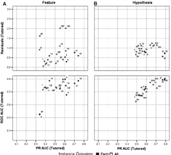
Figure7shows that models that use the each instance (closed squares) grouping generally perform better than those with the all instance grouping (open squares). This effect is very pronounced for hypothesis-triggering, but also observed for feature identification.
A multifactor approach to student model evaluation
Fig. 6 Effect ofnumber of attemptson model performance for Feature identification, (a) and Hypotheses-triggering (b) skills
5.3.2 Model selection
Each of the three metrics provides useful information about the precision and discrim-ination of the model. However, the relative priority of these metrics ultimately depends on the goals of modeling. ROC AUC tells us about the models’ ability to discriminate between student actions, and PR AUC tells us about the averaged precision of cor-rectly identified user actions. Researchers may wish to balance these characteristics in a different way for particular tutoring systems, domains or purposes. For example, if a main objective of the tutoring system is to predict clinical competency after tutoring with the highest possible precision, then PR AUC of the model takes precedence over discrimination. However, if the main objective of the tutoring system is to influence the behavior of the student during tutoring, then discrimination takes precedence over precision.
Fig. 7 Effect ofinstance groupingon model performance for Feature identification, (a) and Hypotheses-triggering (b) skills
of outcomes (high ROC AUC), but also predict outcomes correctly more often and with greater determination (high PR AUC and low residuals). We considered Residuals only when models could not be separated in PR and ROC spaces, based on signifi-cant difference on a majority of the four comparisons (ROC and PR for both feature identification and hypothesis triggering).
A multifactor approach to student model evaluation
Fig. 8 Effect ofmodel topologyon model performance for Feature identification, (a) and Hypotheses-trig-gering (b) skills
and hypothesis triggering) and PR AUC (feature identification and hypothesis trigger-ing). Performance of models using Number of Attempts=All exceeds performance of models using Number of Attempts=First, for ROC (hypothesis triggering) and PR (feature identification and hypothesis triggering), and models using Number of Attempts=First perform better on ROC AUC for feature identification.
Based on our analysis and modeling choices, we selected our final models as fol-lows.
– Model Topology=M2 or M3. – Subgoal Instance Grouping=Each. – Number of Attempts=All.
Table 5 Kruskal–Wallis test results for tutored data. Significant test results are marked in boldface type Factor Metrics Feature identification Hypotheses triggering DF
P-value P-value
Model topology
ROC AUC (M2,M3) > M1 < .001 (M2,M3) > M1 0.258 2 PR AUC (M2,M3) > M1 < .001 (M2,M3) > M1 < .001
Residuals M1 > (M2,M3) 0.011 M1 > (M2,M3) 0.098 Subgoal
instance grouping
ROC AUC Each > All < .001 Each > All 0.003 1
PR AUC Each > All < .001 Each > All < .001
Residuals All > Each 0.703 Each > All < .001
Number of attempts
ROC AUC 1st > All < .001 All > 1st 0.01 1 PR AUC All > 1st < .001 All > 1st < .001
Residuals 1st > All < .001 1st > All 0.005 Figure9depicts multiple comparisons of models based on the results of Tukey– Kramer tests on tutored data. The figure compares performance of one of the two selected models against all other models for each of the three performance metrics. Models selected at the end of Step Two are shown with filled circles. Models used for comparison (#19 for feature identification and #20 for hypothesis triggering) are shown with black filled circle, and the other two selected models (#27 for feature iden-tification and # 28 for hypothesis-triggering) are shown with grey filled circles. Lines depict a 95% confidence interval around the selected models. The best models should have the highest scores in ROC and PR spaces, and the lowest scores in Residuals space. The models #19, 20, 27 and 28 that were pre-selected during the multifactor analysis are among the best in ROC and Residuals spaces for both feature identifi-cation and hypothesis-triggering. In PR space, they are the best models, significantly better than most other models.
5.4 External validity of model selection using post-test and retention-test data
How well does this methodology perform in selecting models that are truly predictive of student performance on the native task after tutoring? We compared models selected using this methodology to post-test data obtained outside of the tutoring environment. This data had not previously been used in model training or testing. The tutored data set that we used for training the models and the post- and retention test data set were not equivalent. Tutored data reflects student interactions with the system, while the test data is obtained without any such interaction. Additionally, the volume of post-and retention test data is much smaller.
Figures10and12show model performance for post-test and retention test respec-tively. The models that we selected in the previous section (shown as closed circles in all graphs) were among the highest performing models on both post-test and retention test data.
A multifactor approach to student model evaluation
Fig. 9 Tukey–Kramer test results on tutored data for individual models for Feature identification (a) and Hypothesis-triggering (b). X-axis—model rank, Y-axis—model number. Filled black circles show models selected on each subplot; filled gray circles show other models selected during multifactor analysis; black open circles with dashed lines show models that are significantly different from selected model; light gray open circles show models that are not significantly different from selected model
Fig. 10 Comparison of selected models compared to other models in predicting post-test data for Feature identification, (a) and Hypotheses-triggering (b) skills
Fig. 11 Residuals for (a) Model 4 and (b) Model 19 on post-test data for each student, where NR=norm of residual for model
A multifactor approach to student model evaluation
Fig. 12 Comparison of selected models compared to other models in predicting retention test data for Feature identification, (a) and Hypotheses-triggering (b) skills
On retention-test hypothesis-triggering data, model 20 has high ROC AUC and PR AUC and residuals in the lower range. Model 28 also has high ROC AUC and PR AUC, although residuals are slightly higher. The equivalent models also perform well for fea-ture identification, although not as consistently across all performance metrics. Model 19 exhibits the highest ROC AUC with the lowest residuals, but has a more average PR AUC. The PR AUC is in the high range for Model 27, but ROC AUC is lower.
tutored data set may not have sufficient opportunity to demonstrate their strengths on a smaller dataset.
6 Discussion
This study described the use of a multifactor approach to student model selection for a complex cognitive task. Our findings have implications for student modeling of diagnostic tasks in medical ITS. Additionally, the evaluation approach we describe may prove generally useful for student model selection using machine learning methods.
6.1 Implications for student modeling of medical diagnostic tasks
Choosing a student modeling formalism for an ITS in a novel domain can be a diffi-cult decision. On the surface, the structure of diagnostic reasoning seems unlike most highly procedural tasks, which have been previously modeled. Diagnostic reasoning requires an array of disparate cognitive skills such as visual search, feature recognition, hypothetico-deductive reasoning, and reasoning under uncertainty. Vast declarative knowledge representations are often brought to bear. The degree to which skills can be broken down into their atomic and conditionally independent sub-skills may be quite limited.
We entertained several approaches to implementing a student model for our task. One approach we considered was to attempt to mirror this diagnostic and task com-plexity within the student model. For example, student models based on Dynamic Bayesian Networks (Conati et al. 2002) were appealing, because there is a long his-tory of modeling medical knowledge with Bayesian networks. However, the size of the knowledge spaces that we routinely work in would quickly prove intractable for this method. The student model must evaluate with sufficient speed to make pedagogic decisions while interacting with the student.
Another option we considered was to limit the model complexity by using a simpler student modeling formalism already known to be highly effective in other domains, such as classic Bayesian Knowledge Tracing. However, some assumptions underly-ing the classical BKT approach seemed in conflict with our experience in cognitive modeling for this domain.
A multifactor approach to student model evaluation
6.1.1 Inclusion of additional hidden states and observed values
Our data supports the use of multiple hidden-state models for student modeling in our domain. Models with three states consistently outperformed those with only two states. Based on our evaluation data, we modified the BKT topology to include hint actions as a third observed outcome in the model. In this approach, hints are considered as a behavior distinct from correct and incorrect actions, but there is no separate node for hints or help.
From a machine learning perspective, adding additional hidden states improves the achievable likelihood of the model. This is because better agreement can be reached by allowing for a different state at every time step. The interpretation of the “meaning” of the hidden node states is very difficult (Murphy 2001), since hidden nodes may have complex interdependencies. Taking this approach produces a model that is less bounded by educational theory, but could have other advantages such as enhanced predictive performance.
6.1.2 Modeling all attempts instead of only first attempts
Our data suggests that modeling multiple attempts within a problem is superior to mod-eling only the first attempt. In classical BKT—the argument against use of multiple attempts is that students who use these systems typically learn from hints between attempts. Therefore, second attempts may provide little useful information. However, we have found that learners in our domain often resist use of hints. Thus, second and third attempts may yield valuable information—particularly because instances of individual skills can be quite different across cases or problems.
6.1.3 Adjusting for non-atomicity of skills
There are two factors in cognitive modeling of medical tasks that make selection of skill granularity a difficult problem. First, medical tasks such as visual diagnostic classifi-cation often have many different classes of skills that may be learned differently. In our case, we distinguish identification of visually represented features and qualities from the exercise of the hypothetico-deductive mechanisms. Second, the enormous range of potential instances of a given skill are difficult to encode into standard production rule systems—which have led us to more general abstract rules that can function across all instances (Crowley and Medvedeva 2006). Given these two inherent ways of subdi-viding skills—at what level of granularity should student skills be modeled? Our data suggests that differentiating both different skill classes (e.g. feature identification and hypothesis-triggering), and instances of these classes may provide useful distinctions.
6.1.4 Modeling forgetting
did on post-test data. Our validation data provided only a one-week interval between post-test and retention test. The relative advantage of the M3 models could be more pronounced with longer time intervals. The benefit of explicitly representing time is that such models could function variably across the long time spans that are needed to develop expertise in such a complex task. Additional work is needed in this area to determine the most predictive models over wider time ranges.
6.1.5 Predicting student actions as opposed to knowledge states
A fundamental difference in our resulting approach is to attempt to predict student action outcome (observable node) rather than knowledge state (hidden node). The benefit of this approach is that it gives us (1) more flexibility in designing pedagogic approaches to student actions because requests for help can also be predicted in addi-tion to correct and incorrect answers, and (2) a greater ability to compare models directly because the predicted values relate to observable outcomes which can be compared to other data such as test performance. Predicting competency in future actions is particularly important in high-risk tasks such as medicine, nuclear power plant management and plane piloting. ITS which simulate these tasks have the dual responsibility of education and assessment.
6.1.6 Learning conditional probabilities directly from data
Our decision to emphasize prediction led us to use a machine learning approach to determine prior and conditional probabilities for the student model. An additional fac-tor in favor of this decision was that, unlike other ITS domains, very little is known about the natural frequencies of these intermediate steps because there is little relevant work on cognitive modeling in diagnostic reasoning.
6.2 Evaluation approach
The methodology we used to evaluate models is general and could be used by other researchers to identify appropriate student models for their novel domains, systems, or pedagogic approaches. The current state-of-the-art for student modeling is chang-ing. More recent efforts have focused on using machine learning techniques to learn model parameters as an alternative to expert estimation (Jonsson et al. 2005;Chang et al. 2006). Machine learning approaches necessitate the development of method-ologies for evaluating large numbers of potential models that result from this ap-proach.
A multifactor approach to student model evaluation
predicting performance. We used three metrics: (1) Precision-Recall area under curve (PR AUC), our measure of the models’ ability to predict, (2) Area under Receiver Operating Characteristic curve (ROC AUC), our measure of the models’ ability to discriminate different outcomes of user actions (three in our case), and (3) Resid-uals, a measurement of the difference between test result and prediction. Based on the metrics, best models were selected in the following way. For each factor/dimen-sion of the dataset we selected one level of the factor whose models perform better. An intersection of the best factor levels was used as the best configuration for the models.
6.2.1 Tradeoffs
An inherent limitation to any student modeling within an ITS is that we do not know when incorrect answers are slips and when correct answers are guesses. Classical BKT takes the approach of empirically setting values in the confusion matrix of the HMM. (Corbett and Anderson 1995;VanLehn and Niu 2001;Shang et al. 2001). Because slips and guesses occur—no single model can predict student actions perfectly. There will always be uncertainty resulting in lower values of ROC AUC and PR AUC metrics.
ROC AUC that is less than 0.85 is considered to be a noisy area where it is diffi-cult to achieve sufficient discrimination from models. Because students slip and guess with any action, it is simply not possible to achieve a perfectly discriminating model. Although some models can be excluded early because their ROC AUC metrics are very low, most models we have considered (and in fact most models we are likely to ever consider) fall into this are between 0.7 and 0.81 ROC AUC. Therefore we need to use other metrics to separate them.
Precision-Recall Area Under Curve (PR AUC) gives us an additional metric to separate these models. In the context of our models, PR is a measure of the precision of model performance in predicting the next student action. Precision itself is a widely used measure, and can be directly compared to later performance (for example on post-tests). PR AUC enables model choice within the limits of the inherent tradeoff between precision and recall of a model. Different models may have the same ROC AUC and different PR AUC, or may have the same PR AUC and different ROC AUC. PR AUC alone is not a sufficient metric because it is very sensitive to the way data is aggregated.
6.3 Conclusions
Alteration of some basic assumptions of classical BKT yields student models that are more predictive of student performance. The methodology used to select these models can be applied to other ITS in novel domains.
6.4 Future work
This project is part of our ongoing work to develop a scalable, general architecture for tutoring medical tasks. The modified BKT model we selected has already been implemented into the SlideTutor system and is now being used by students in our eval-uation studies. In future work, we will test the ability of an inspectable student model to improve student self-assessment and certainty on diagnostic tasks. Our pedagogic model will use the modified BKT model to select cases and appropriate instructional interventions.
An important finding of our work was that even the best models we evaluated (e.g. Model #19 for features, ROC AUC=0.80; or model #20 for hypotheses, ROC AUC=0.81) leave significant room for improvement. Future modeling work in our laboratory will assess the potential benefits of slightly more complex models, focusing on three specific areas: inter-skill dependencies, forgetting, and visual search.
Inter-skill dependencies move us away from another basic assumption of clas-sical BKT—conditional independence of skills. Cognitive ITS usually model tasks as a set of elemental sub-skills, in keeping with current theories of skill acquisition such as ACT-R. But, many sub–skills in diagnostic tasks are difficult to model at this level, and may require skill–skill dependencies in order to capture the inherent complexity.
The current study suggests that time may be an important additional factor in this skill acquisition process that should be included. Skill acquisition in this domain is often accompanied by a concomitant increase in declarative knowledge. Students typ-ically work on acquiring skills in specific areas of the domain periodtyp-ically over the course of many years. In future work, we will more carefully study the natural history of forgetting as skill senescence and determine whether addition of a time variable to our models improves prediction over longer time spans of ITS use.
Visual search is a critical component of this skill which we normally capture in our ITS through use of a virtual microscope. To date, we have not included this informa-tion in our models. But aspects of visual search may be extremely helpful in further improving our prediction of feature learning. For example, variables such as gaze-time and fixations per unit space could provide information about how well students are attending to visual features as they work in the tutoring system. Inclusion of such fea-tures may be guided by existing theories of skill acquisition, which include lower-level cognitive processes such as perception and attention (Byrne et al. 1998).
A multifactor approach to student model evaluation References
Anderson, J.: Rules of the Mind. Lawrence Erlbaum Associates, Hillsdale, NJ (1993)
Anderson, J., Schunn, C. : Implications of the ACT-R learning theory: no magic bullets. In: Glaser, R. (ed.) Advances in Instructional Psychology: Educational Design and Cognitive Science, vol. 5, pp. 1–34. Erlbaum, Mahwah, NJ (2000)
Anderson, J.R., Corbett, A.T., Koedinger, K.R., Pelletier, R.: Cognitive tutors: lessons learned. J. Learn. Sci.4(2), 167–207 (1995)
Atkinson, R., Shiffrin, R.: Human memory: a proposed system and its control processes. In: Spence, K.W., Spence, J.T. (eds.) The Psychology of Learning and Motivation: Advances in Research and Theory, vol. 2, pp. 742–775.Academic Press, New York (1968)
Beck, J., Sison, J.: Using knowledge tracing to measure student reading proficiencies. In: Proceedings of the 7th International Conference on Intelligent Tutoring Systems, pp. 624–634. Springer-Verlag, Maceio, Brazil (2004)
Brand, M., Oliver, N., Pentland, A.: Coupled hidden Markov models for complex action recognition. In: Proceedings of the IEEE International Conference on Computer Vision and Pattern Recognition, pp. 994–999. San Juan, Puerto Rico (1997)
Byrne, M.D.: Perception and action. In: Anderson, J.R., Lebiére, C. (eds.) Atomic Components of Thought, pp. 167–200. Erlbaum, Hillsdale (1998)
Chang, K., Beck, J., Mostow, J., Corbett, A.: Does help help? A Bayes net approach to modeling tutor interventions. In: Proceedings of the 21st Annual Meeting of the American Association for Artificial Intelligence, pp. 41–46. Boston, MA (2006)
Clancey, W.: Methodology for building an intelligent tutoring system. In: Kintsch, W., Miller, H., Poison, P. (eds.) Methods and Tactics in Cognitive Science, pp. 51–84. Erlbaum, Hillsdale (1984)
Clancey, W., Letsinger, R.: NEOMYCIN: reconfiguring a rule based expert system for application to teach-ing. In: Proceedings of the Seventh International Joint Conference on AI, pp. 829–835. Vancouver, BC, Canada (1981)
Conati, C., Zhao, X.: Building and evaluating an intelligent pedagogical agent to improve the effective-ness of an educational game. In: Proceedings of the 9th International Conference on Intelligent User Interface, pp. 6–13. Funchal, Madeira, Portugal (2004)
Conati, C., Gertner, A., VanLehn, K.: Using Bayesian networks to manage uncertainty in student model-ing. J. User Model. User-Adap. Interac.12(4), 371–417 (2002)
Corbett, A., Anderson, J.: Knowledge tracing: modeling the acquisition of procedural knowledge. User Model. User-Adap. Interac.4, 253–278 (1995)
Crowley, R., Medvedeva, O.: An intelligent tutoring system for visual classification problem solving. Artif. Intell. Med.36(1), 85–117 (2006)
Crowley, R., Naus, G., Stewart, J., Friedman, C.: Development of visual diagnostic expertise in pathology – an information processing study. J. Am. Med. Inform. Assoc.10(1), 39–51 (2003)
Crowley, R., Legowski, E., Medvedeva, O., Tseytlin, E., Roh, E., Jukic, D.: Evaluation of an Intelligent Tutoring system in pathology: effects of external representation on performance gains, metacognition, and acceptance. J. Am. Med. Inform. Assoc.14(2), 182–190 (2007)
Davis, J., Goadrich, M.: The relationship between Precision-Recall and ROC curves. In: Proceedings of the 23rd International Conference on Machine Learning, vol. 148, pp. 233–240. Pittsburgh, PA (2006) Ephraim, Y., Roberts, W.: Revisiting autoregressive hidden Markov modeling of speech signals. IEEE Sig.
Proc. Lett.12, 166–169 (2005)
Fawcett, T.: Graphs: notes and practical considerations for data mining researchers. Tech Reports HPL-2003-4. HP Laboratories, Palo Alto, CA (2003)
Ferguson, K., Arroyo, I., Mahadevan, S., Woolf, B., Barto, A.: Improving intelligent tutoring systems: Using EM to learn student skill levels, Intelligent Tutoring Systems, pp. 453–462. Springer-Verlag, Jhongli, Taiwan (2006)
Fogarty, J., Baker, R.S., Hudson, S.: Case studies in the use of ROC curve analysis for sensor-based esti-mates in Human Computer Interaction. In: Proceedings of Graphics Interface, pp. 129–136. Victoria, British Columbia, Canada (2005)
Jastrzembski, T., Gluck, K., Gunzelmann, G.: Knowledge tracing and prediction of future trainee per-formance. In: Proceedings of the 2006 Interservice/Industry Training, Simulation, and Education Conference, pp. 1498–1508. National Training Systems Association, Orlando, FL (2006)
Jonsson, A., Johns, J., Mehranian, H., Arroyo, I., Woolf, B., Barto, A., Fisher, D., Mahadevan, S.: Evaluat-ing the feasibility of learnEvaluat-ing student models from data. In: AAAI05 Workshop on Educational Data Mining, pp. 1–6. Pittsburgh, PA (2005)
Kuenzer, A., Schlick, C., Ohmann, F., Schmidt, L., Luczak, H.: An empirical study of dynamic Bayesian networks for user modeling. In: UM’01 Workshop on Machine Learning for User Modeling, pp. 1–10. Sonthofen, Germany (2001)
Mayo, M., Mitrovic, A.: Optimizing ITS behavior with Bayesian networks and decision theory. Int. J. Artifi. Intell. Educ.12, 124–153 (2001)
Medvedeva, O., Chavan, G., Crowley, R.: A data collection framework for capturing ITS data based on an agent communication standard. In: Proceedings of the 20th Annual Meeting of the American Association for Artificial Intelligence, pp. 23–30. Pittsburgh, PA (2005)
Moore, D., McCabe, G.: Introduction to the Practice of Statistics. W.H. Freeman and Company, New York (1993)
Murphy, K.: The Bayes Net Toolbox for Matlab. Computing Science and Statistics, vol. 33, pp. 1–20. URL:
http://www.bnt.sourceforge.net(Accessed on December 6, 2008) (2001)
Provost, F., Fawcett, T., Kohavi, R.: The case against accuracy estimation for comparing induction algo-rithms. In: Proceeding of the 15th International Conference on Machine Learning, pp. 445–453. San Francisco, CA (1998)
Reye, J.: Student modeling based on belief networks. Int. J. Artif. Intell. Educ.14, 1–33 (2004)
Seidemann, E., Meilijson, I., Abeles, M., Bergman, H., Vaadia, E.: Simultaneously recorded single units in the frontal cortex go through sequences of discrete and stable states in monkeys performing a delayed localization task. J. Neurosci.16(2), 752–768 (1996)
Shang, Y., Shi, H., Chen, S.: An intelligent distributed environment for active learning. J. Educ. Resour. Comput.1(2), 1–17 (2001)
VanLehn, K., Niu, Z.: Bayesian student modeling, user interfaces and feedback: a sensitivity analysis. Int. J. Artif. Intell. Educ.12, 154–184 (2001)
Zukerman, I., Albrecht, D.W., Nicholson, A.E.: Predicting users’ requests on the WWW. In: Proceedings of the Seventh International Conference on User Modeling, (UM-99), pp. 275–284. Banff, Canada (1999) Authors’ vitae
Michael V. Yudelsonis a PhD candidate in the School of Information Sciences at the University of Pitts-burgh. He received his M.S. degree in computer-aided design from Ivanovo State Power University, Ivanovo, Russia in 2001. His research interests include adaptive hypermedia and service architectures for personali-zation, user modeling, and human-computer interaction. He is the recipient of the James Chen Student Paper Award at the International Conference on User Modeling 2007 for work on a service architecture for user modeling, and the Doctoral Consortium Paper award at the International Conference on AI in Education 2007 for work on learning factor analysis.
Olga P. Medvedevais a senior software engineer in the Department of Biomedical Informatics at the Uni-versity of Pittsburgh School of Medicine. She received her master’s degrees in Astrophysics from Moscow State University, and in Radiophysics from the Russian Academy of Science. Since 2001 she has been the architect of the SlideTutor project, where she works on many of the artificial intelligence aspects of the system including student modeling.