II. More importantly, the use of the unit step function (Heaviside function in Sec. 6.3) and Dirac’s delta (in Sec. 6.4) make the method particularly powerful for problems with inputs (driving forces) that have discontinuities or represent short impulses

203

C H A P T E R

6

Laplace Transforms

Laplace transforms are invaluable for any engineer’s mathematical toolbox as they make solving linear ODEs and related initial value problems, as well as systems of linear ODEs, much easier. Applications abound: electrical networks, springs, mixing problems, signal processing, and other areas of engineering and physics.

The process of solving an ODE using the Laplace transform method consists of three steps, shown schematically in Fig. 113:

Step 1.The given ODE is transformed into an algebraic equation, called the subsidiary equation.

Step 2.The subsidiary equation is solved by purely algebraic manipulations.

Step 3.The solution in Step 2 is transformed back, resulting in the solution of the given problem.

Fig. 113. Solving an IVP by Laplace transforms

The key motivation for learning about Laplace transforms is that the process of solving an ODE is simplified to an algebraic problem (and transformations). This type of mathematics that converts problems of calculus to algebraic problems is known as operational calculus. The Laplace transform method has two main advantages over the methods discussed in Chaps. 1–4:

I. Problems are solved more directly: Initial value problems are solved without first determining a general solution. Nonhomogenous ODEs are solved without first solving the corresponding homogeneous ODE.

II. More importantly, the use of the unit step function(Heaviside functionin Sec. 6.3) and Dirac’s delta(in Sec. 6.4) make the method particularly powerful for problems with inputs (driving forces) that have discontinuities or represent short impulses or complicated periodic functions.

Solution of the

IVP Solving

AP by Algebra AP

Algebraic Problem IVP

Initial Value

Prerequisite: Chap. 2

Sections that may be omitted in a shorter course: 6.5, 6.7 References and Answers to Problems: App. 1 Part A, App. 2.

6.1

Laplace Transform. Linearity.

First Shifting Theorem (

s

_-Shifting)

In this section, we learn about Laplace transforms and some of their properties. Because Laplace transforms are of basic importance to the engineer, the student should pay close attention to the material. Applications to ODEs follow in the next section.

Roughly speaking, the Laplace transform, when applied to a function, changes that function into a new function by using a process that involves integration. Details are as follows.

If is a function defined for all , its Laplace transform1_{is the integral of} times from to . It is a function of s, say, , and is denoted by ; thus

(1)

Here we must assume that is such that the integral exists (that is, has some finite value). This assumption is usually satisfied in applications—we shall discuss this near the end of the section.

f(t)

F(s)l₍f˛)

冮

ⴥ

0

eⴚst_{f(t) dt.}

l_(f)

F(s)

t₀

eⴚst t f(t)

₀ f(t)

Topic Where to find it

ODEs, engineering applications and Laplace transforms Chapter 6 PDEs, engineering applications and Laplace transforms Section 12.11 List of general formulas of Laplace transforms Section 6.8 List of Laplace transforms and inverses Section 6.9

Note: Your CAS can handle most Laplace transforms.

1_{PIERRE SIMON MARQUIS DE LAPLACE (1749–1827), great French mathematician, was a professor in}

Paris. He developed the foundation of potential theory and made important contributions to celestial mechanics, astronomy in general, special functions, and probability theory. Napoléon Bonaparte was his student for a year. For Laplace’s interesting political involvements, see Ref. [GenRef2], listed in App. 1.

The powerful practical Laplace transform techniques were developed over a century later by the English electrical engineer OLIVER HEAVISIDE (1850–1925) and were often called “Heaviside calculus.”

We shall drop variables when this simplifies formulas without causing confusion. For instance, in (1) we wrote instead of and in instead of lⴚ1₍ .

F)(t) (1*) lⴚ1₍

F)

l(f)(s)

l( f )

SEC. 6.1 Laplace Transform. Linearity. First Shifting Theorem (s_{-Shifting) 205}

Not only is the result called the Laplace transform, but the operation just described, which yields from a given , is also called the Laplace transform. It is an “integral transform”

with “kernel”

Note that the Laplace transform is called an integral transform because it transforms (changes) a function in one space to a function in another space by a process of integration that involves a kernel. The kernel or kernel function is a function of the variables in the two spaces and defines the integral transform.

Furthermore, the given function in (1) is called the inverse transformof and is denoted by ; that is, we shall write

(1*)

Note that (1) and (1*) together imply and .

Notation

Original functions depend on t and their transforms on s—keep this in mind! Original functions are denoted by lowercase lettersand their transforms by the same letters in capital, so that denotes the transform of , and denotes the transform of , and so on.

E X A M P L E 1 Laplace Transform

Let when . Find .

Solution. From (1) we obtain by integration

.

Such an integral is called an improper integraland, by definition, is evaluated according to the rule

.

Hence our convenient notation means

.

We shall use this notation throughout this chapter.

E X A M P L E 2 Laplace Transform of the Exponential Function

Let when , where ais a constant. Find .

Solution. Again by (1),

Must we go on in this fashion and obtain the transform of one function after another directly from the definition? No! We can obtain new transforms from known ones by the use of the many general properties of the Laplace transform. Above all, the Laplace transform is a “linear operation,” just as are differentiation and integration. By this we mean the following.

T H E O R E M 1 Linearity of the Laplace Transform

The Laplace transform is a linear operation; that is, for any functions and whose transforms exist and any constants a and b the transform of

exists, and

P R O O F This is true because integration is a linear operation so that (1) gives

E X A M P L E 3 Application of Theorem 1: Hyperbolic Functions

Find the transforms of and .

Solution. Since and , we obtain from Example 2 and

Theorem 1

E X A M P L E 4 Cosine and Sine

Derive the formulas

, .

Solution. We write and . Integrating by parts and noting that the integral-free parts give no contribution from the upper limit , we obtain

SEC. 6.1 Laplace Transform. Linearity. First Shifting Theorem (s_{-Shifting) 207}

By substituting into the formula for on the right and then by substituting into the formula for on the right, we obtain

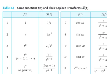
Basic transformsare listed in Table 6.1. We shall see that from these almost all the others can be obtained by the use of the general properties of the Laplace transform. Formulas 1–3 are special cases of formula 4, which is proved by induction. Indeed, it is true for because of Example 1 and . We make the induction hypothesis that it holds for any integer and then get it for directly from (1). Indeed, integration by parts first gives

.

Now the integral-free part is zero and the last part is times . From this and the induction hypothesis,

This proves formula 4.

in formula 5 is the so-called gamma function [(15) in Sec. 5.5 or (24) in App. A3.1]. We get formula 5 from (1), setting :

where . The last integral is precisely that defining , so we have , as claimed. (CAUTION! has in the integral, not .) Note the formula 4 also follows from 5 because for integer . Formulas 6–10 were proved in Examples 2–4. Formulas 11 and 12 will follow from 7 and 8 by “shifting,” to which we turn next.

s

_{-Shifting: Replacing}

s

_by

_{in the Transform}

The Laplace transform has the very useful property that, if we know the transform of we can immediately get that of , as follows.

T H E O R E M 2 First Shifting Theorem, s_-Shifting

If has the transform (where for some k), then has the transform (where . In formulas,

or, if we take the inverse on both sides,

.

P R O O F We obtain by replacing swith in the integral in (1), so that

.

If exists (i.e., is finite) for sgreater than some k, then our first integral exists for . Now take the inverse on both sides of this formula to obtain the second formula

in the theorem. (CAUTION! in but

E X A M P L E 5 s_{-Shifting: Damped Vibrations. Completing the Square}

From Example 4 and the first shifting theorem we immediately obtain formulas 11 and 12 in Table 6.1,

For instance, use these formulas to find the inverse of the transform

l( f ) 3s137

s2_2s401.

l{eatcos vt} sa

(sa)2

v2

, l{eatsin vt} v

(sa)2

v2

.

䊏 _{a in e}at_f(t).)

F(s_{a) a}

s_ak F(s)

F(s_a)

冮

ⴥ

0

eⴚ(sⴚa)t_{f(t) dt}

冮

ⴥ

0

eⴚst_3eat_{f(t)4 dtl{e}at_f(t)}

s_a F(s_a)

eatf(t)lⴚ1_{F(sa)}

l_{eat_f(t)}F(sa) s_ak)

F(s_a)

eatf(t) s_k

F(s) f(t)

eatf(t)

f(t),

s

a

n_{0 (n1)n!}

xa1 xa

_{(a1) (a1)>s}a1

_(a1) s₀

l_(ta₎

冮

ⴥ

0

eⴚst_ta_dt

冮

ⴥ

0 eⴚx_ax

sb a

dx

s

1 sa1

冮

ⴥ

0

eⴚx_xa_dx st_x

Solution. Applying the inverse transform, using its linearity (Prob. 24), and completing the square, we obtain

We now see that the inverse of the right side is the damped vibration (Fig. 114)

䊏

f(t)eⴚt_{(3 cos 20t7 sin 20}t).

flⴚ1_b3(s1)140

(s₁₎2₄₀₀r

₃lⴚ1_b s1

(s₁₎2₂₀2r

₇lⴚ1_b 20

(s₁₎2₂₀2r.

SEC. 6.1 Laplace Transform. Linearity. First Shifting Theorem (s_{-Shifting) 209}

t 0

4

–4

–6 2

–2 6

1.0 1.5 2.0 2.5 3.0 0.5

Fig. 114. Vibrations in Example 5

Existence and Uniqueness of Laplace Transforms

This is not a big practicalproblem because in most cases we can check the solution of an ODE without too much trouble. Nevertheless we should be aware of some basic facts.

A function has a Laplace transform if it does not grow too fast, say, if for all and some constants Mand kit satisfies the “growth restriction”

(2)

(The growth restriction (2) is sometimes called “growth of exponential order,” which may be misleading since it hides that the exponent must be kt, not or similar.)

need not be continuous, but it should not be too bad. The technical term (generally used in mathematics) is piecewise continuity. is piecewise continuouson a finite interval where fis defined, if this interval can be divided into finitely many subintervals in each of which fis continuous and has finite limits as tapproaches either endpoint of such a subinterval from the interior. This then gives finite jumps as in Fig. 115 as the only possible discontinuities, but this suffices in most applications, and so does the following theorem.

atb

f(t) f(t)

kt2 ƒf(t)ƒ Mekt.

t₀ f(t)

t

a b

T H E O R E M 3 Existence Theorem for Laplace Transforms

If is defined and piecewise continuous on every finite interval on the semi-axis and satisfies (2)for all and some constants M and k, then the Laplace transform exists for all

P R O O F Since is piecewise continuous, is integrable over any finite interval on the t-axis. From (2), assuming that (to be needed for the existence of the last of the following integrals), we obtain the proof of the existence of from

Note that (2) can be readily checked. For instance, (because is a single term of the Maclaurin series), and so on. A function that does not satisfy (2) for any M and k is (take logarithms to see it). We mention that the conditions in Theorem 3 are sufficient rather than necessary (see Prob. 22).

Uniqueness. If the Laplace transform of a given function exists, it is uniquely determined. Conversely, it can be shown that if two functions (both defined on the positive real axis) have the same transform, these functions cannot differ over an interval of positive length, although they may differ at isolated points (see Ref. [A14] in App. 1). Hence we may say that the inverse of a given transform is essentially unique. In particular, if two continuousfunctions have the same transform, they are completely identical.

et2

Find the transform. Show the details of your work. Assume that a,b, are constants.

17. Table 6.1. Convert this table to a table for finding inverse transforms (with obvious changes, e.g.,

etc).

18. Using in Prob. 10, find where

if and if

19. Table 6.1. Derive formula 6 from formulas 9 and 10.

20. Nonexistence. Show that does not satisfy a condition of the form (2).

21. Nonexistence. Give simple examples of functions (defined for all that have no Laplace transform.

22. Existence. Show that [Use (30) in App. 3.1.] Conclude from this that the conditions in Theorem 3 are sufficient but not necessary for the existence of a Laplace transform.

SEC. 6.2 Transforms of Derivatives and Integrals. ODEs 211

23. Change of scale. If and c is any positive constant, show that (Hint: Use (1).) Use this to obtain

24. Inverse transform. Prove that is linear. Hint: Use the fact that is linear.

25–32 INVERSE LAPLACE TRANSFORMS

Given find a,b, L, nare constants. Show the details of your work.

25. 26.

In Probs. 33–36 find the transform. In Probs. 37–45 find the inverse transform. Show the details of your work.

33. 34.

6.2

Transforms of Derivatives and Integrals.

ODEs

The Laplace transform is a method of solving ODEs and initial value problems. The crucial idea is that operations of calculus on functions are replaced by operations of algebra on transforms. Roughly, differentiationof will correspond to multiplicationof by s(see Theorems 1 and 2) and integrationof to division of by s. To solve ODEs, we must first consider the Laplace transform of derivatives. You have encountered such an idea in your study of logarithms. Under the application of the natural logarithm, a product of numbers becomes a sum of their logarithms, a division of numbers becomes their difference of logarithms (see Appendix 3, formulas (2), (3)). To simplify calculations was one of the main reasons that logarithms were invented in pre-computer times.

T H E O R E M 1 Laplace Transform of Derivatives

The transforms of the first and second derivatives of satisfy (1)

(2)

Formula (1) holds if is continuous for all and satisfies the growth restriction(2)in Sec. 6.1and is piecewise continuous on every finite interval on the semi-axis Similarly,(2) holds if f and are continuous for all and satisfy the growth restriction and is piecewise continuous on every finite interval on the semi-axis t_0.

P R O O F We prove (1) first under the additional assumptionthat is continuous. Then, by the definition and integration by parts,

Since fsatisfies (2) in Sec. 6.1, the integrated part on the right is zero at the upper limit when and at the lower limit it contributes The last integral is It exists for because of Theorem 3 in Sec. 6.1. Hence exists when and (1) holds. If is merely piecewise continuous, the proof is similar. In this case the interval of integration of must be broken up into parts such that is continuous in each such part. The proof of (2) now follows by applying (1) to and then substituting (1), that is

Continuing by substitution as in the proof of (2) and using induction, we obtain the following extension of Theorem 1.

T H E O R E M 2 Laplace Transform of the Derivative of Any Order

Let be continuous for all and satisfy the growth restriction (2)in Sec.6.1. Furthermore, let be piecewise continuous on every finite interval on the semi-axis . Then the transform of satisfies

(3)

E X A M P L E 1 Transform of a Resonance Term (Sec. 2.8)

Let Then Hence

by (2),

thus

E X A M P L E 2 Formulas 7 and 8 in Table 6.1, Sec. 6.1

This is a third derivation of and ; cf. Example 4 in Sec. 6.1. Let Then From this and (2) we obtain

By algebra,

Similarly, let Then From this and (1) we obtain

Hence,

Laplace Transform of the Integral of a Function

Differentiation and integration are inverse operations, and so are multiplication and division. Since differentiation of a function (roughly) corresponds to multiplication of its transform

by s, we expect integration of _f(t)to correspond to division of l_{( f )}by s:

l_{( f )}

f(t)

䊏

l(sin vt)v

sl(cos vt)

v

s2v2.

l(gr)_sl(g) _vl(cos vt).

g(0)_{0, grv cos vt.}

g_{sin vt.}

l_{(cos v}t) s

s2

v2

.

l₍ fs)s2_{l( f )s}

v2l₍ f ).

f(0)_1, fr(0)_0, fs(t) v2 cos vt.

f(t)_cos vt.

l_(sin vt)

l_(cos vt)

䊏

l₍ f )l₍t sin vt) 2vs

(s2v2)2. l₍ fs)₂v s

s2v2

v2l₍ f )s2l₍ f ),

f(0)0, fr(t)sin vtvt cos vt, fr(0)0, fs2v cos vtv2t sin vt.

f(t)t sin vt.

l_{( f}(n)₎snl_{( f )}snⴚ1_f(0)snⴚ2_f

r

(0) Á _f(nⴚ1)_(0). f(n)

t₀

f(n)

t₀ f, f

_r

,Á, f(nⴚ1)

f(n)

䊏

l_{( f}

_s

₎sl_{( f}

_r

₎f

_r

(0)s3sl_{( f )}f(0)4s2l_{( f )}sf(0)f

_r

(0). f

_s

f

_r

f

_r

f

_r

sk

l_{( f}

_r

₎

sk

l_{( f ).}

f(0). s_k,

l_{( f}

_r

₎

冮

ⴥ

0

eⴚst_f

_r

_{(t) dt3e}ⴚst_f(t)4` ⴥ

0 s

冮

ⴥ

0

eⴚst_{f(t) dt.}

T H E O R E M 3 Laplace Transform of Integral

Let denote the transform of a function which is piecewise continuous for and satisfies a growth restriction (2), Sec. 6.1.Then, for and

(4) thus

P R O O F Denote the integral in (4) by Since is piecewise continuous, is continuous, and (2), Sec. 6.1, gives

This shows that also satisfies a growth restriction. Also, except at points at which is discontinuous. Hence is piecewise continuous on each finite interval and, by Theorem 1, since (the integral from 0 to 0 is zero)

Division by sand interchange of the left and right sides gives the first formula in (4), from which the second follows by taking the inverse transform on both sides.

E X A M P L E 3 Application of Theorem 3: Formulas 19 and 20 in the Table of Sec. 6.9

Using Theorem 3, find the inverse of and

Solution. From Table 6.1 in Sec. 6.1 and the integration in (4) (second formula with the sides interchanged) we obtain

This is formula 19 in Sec. 6.9. Integrating this result again and using (4) as before, we obtain formula 20 in Sec. 6.9:

It is typical that results such as these can be found in several ways. In this example, try partial fraction reduction.

Differential Equations, Initial Value Problems

Let us now discuss how the Laplace transform method solves ODEs and initial value problems. We consider an initial value problem

(5) y

s

_ay

_r

_{byr(t), y(0)K0, y}

_r

_(0)K1

where aand bare constant. Here is the given input (driving force) applied to the mechanical or electrical system and is the output(response to the input) to be obtained. In Laplace’s method we do three steps:

Step 1. Setting up the subsidiary equation.This is an algebraic equation for the transform obtained by transforming (5) by means of (1) and (2), namely,

where Collecting the Y-terms, we have the subsidiary equation

Step 2. Solution of the subsidiary equation by algebra.We divide by and use the so-called transfer function

(6)

(Qis often denoted by H, but we need Hmuch more frequently for other purposes.) This gives the solution

(7)

If this is simply ; hence

and this explains the name of Q. Note that Q depends neither on r(t) nor on the initial conditions(but only on aand b).

Step 3. Inversion of Y to obtain We reduce (7) (usually bypartial fractions as in calculus) to a sum of terms whose inverses can be found from the tables (e.g., in Sec. 6.1 or Sec. 6.9) or by a CAS, so that we obtain the solution of (5). E X A M P L E 4 Initial Value Problem: The Basic Laplace Steps

Solve

Solution. Step 1. From (2) and Table 6.1 we get the subsidiary equation thus

Step 2.The transfer function is and (7) becomes

Simplification of the first fraction and an expansion of the last fraction gives

Y 1

s₁a

1

s2₁

1

s2b.

Y(s1)Q 1

s2

Q s1

s21

1

s2(s21).

Q_1>(s2_1),

(s21)Ys11>s2.

s2Ysy(0)yr(0)Y1>s2,

3with Yl_(y)4

ysyt, y(0)1, yr(0)1.

y(t)lⴚ1_(Y) yⴝllⴚ1(Y).

Q Y

R

l_(output) l_(input)

Y_RQ

y(0)_y

_r

_(0)0,

Y(s)_3(sa)y(0)y

_r

_{(0)4Q(s)R(s)Q(s).}

Q(s) 1

s2asb

1

(s1_2a)2_b1_4a2.

s2asb (s2_{asb)Y(sa)y(0)y}

r

(0)_R(s). R(s)l_(r).

3s2Y_sy(0)y

_r

(0)4a3sY_y(0)4bY_R(s) Yl_(y)

Step 3. From this expression for Yand Table 6.1 we obtain the solution

The diagram in Fig. 116 summarizes our approach. 䊏

y(t)lⴚ1₍

Y)lⴚ1

e_s1₁fl

ⴚ1

e_s21₁flⴚ 1

e_s12fe

t_{sinh tt.}

SEC. 6.2 Transforms of Derivatives and Integrals. ODEs 215

t-space s-space

Given problem y" – y = t

y(0) = 1 y'(0) =1

Solution of given problem y(t) = et _{+ sinh t – t}

Subsidiary equation

Solution of subsidiary equation (s2 _{– 1)Y = s + 1 + 1/s}2

1 s – 1

1 s2 _{– 1}

1 s2

Y = + –

Fig. 116. Steps of the Laplace transform method

E X A M P L E 5 Comparison with the Usual Method

Solve the initial value problem

Solution. From (1) and (2) we see that the subsidiary equation is thus

The solution is

Hence by the first shifting theorem and the formulas for cos and sin in Table 6.1 we obtain

This agrees with Example 2, Case (III) in Sec. 2.4. The work was less.

Advantages of the Laplace Method

1. Solving a nonhomogeneous ODE does not require first solving the homogeneous ODE.See Example 4.

2. Initial values are automatically taken care of.See Examples 4 and 5. 3. Complicated inputs (right sides of linear ODEs) can be handled very

efficiently,as we show in the next sections. r(t)

䊏

eⴚ0.5t_{(0.16 cos 2.96t0.027 sin 2.96t).}

y(t)lⴚ1₍

Y)_eⴚt>2 _{a0.16 cos} B

35 4 t

0.08

1 2235

sin _B35 4 tb

Y0.16(s 1)

s2s₉

0.16(s

1₂)0.08 (s1₂₎235₄ .

(s2s9)Y0.16(s1).

s2Y0.16ssY0.169Y0,

E X A M P L E 6 Shifted Data Problems

This means initial value problems with initial conditions given at some instead of For such a problem set so that gives and the Laplace transform can be applied. For instance, solve

Solution. We have and we set Then the problem is

where Using (2) and Table 6.1 and denoting the transform of by we see that the subsidiary equation of the “shifted” initial value problem is

thus

Solving this algebraically for we obtain

The inverse of the first two terms can be seen from Example 3 (with and the last two terms give and

Now so that the answer (the solution) is

䊏

1–11 INITIAL VALUE PROBLEMS (IVPS)

Solve the IVPs by the Laplace transform. If necessary, use partial fraction expansion as in Example 4 of the text. Show all details.

12–15 SHIFTED DATA PROBLEMS

Solve the shifted data IVPs by the Laplace transform. Show the details.

12.

13.

14.

15.

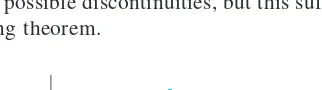
22. PROJECT. Further Results by Differentiation.

Proceeding as in Example 1, obtain

(a)

and from this and Example 1: (b)formula 21, (c)22,

(d)23 in Sec. 6.9,

(e)

(f )

23–29 INVERSE TRANSFORMS BY INTEGRATION

Using Theorem 3, find f(t) if equals:

23. 24.

25. 26.

27. 28.

29. 1

s3as2

3s4

s4_k2 s2 s1

s4_9s2

1

s4_s2

1

s(s2_v2₎

20 s32ps2 3

s2s>4

l_(F) l(t sinh at) 2as

(s2a2)2.

l(t cosh at) s

2

a2 (s2a2)2,

l(t cos vt) s

2

v2

(s2v2)2

SEC. 6.3 Unit Step Function (Heaviside Function). Second Shifting Theorem (t_{-Shifting) 217} 30. PROJECT. Comments on Sec. 6.2. (a) Give reasons why Theorems 1 and 2 are more important than Theorem 3.

(b) Extend Theorem 1 by showing that if is continuous, except for an ordinary discontinuity (finite jump) at some the other conditions remaining as in Theorem 1, then (see Fig. 117)

(1*)

(c) Verify (1*) for if and 0 if

(d) Compare the Laplace transform of solving ODEs with the method in Chap. 2. Give examples of your own to illustrate the advantages of the present method (to the extent we have seen them so far).

t_1.

0t1 f(t)eⴚt

l_(fr)sl_{( f )f(0)3f(a0)f(a0)4e}ⴚas_. t_{a (0),}

f(t)

6.3

Unit Step Function (Heaviside Function).

Second Shifting Theorem (

t

_-Shifting)

This section and the next one are extremely important because we shall now reach the point where the Laplace transform method shows its real power in applications and its superiority over the classical approach of Chap. 2. The reason is that we shall introduce two auxiliary functions, the unit step functionor Heaviside function (below) and Dirac’s delta (in Sec. 6.4). These functions are suitable for solving ODEs with complicated right sides of considerable engineering interest, such as single waves, inputs (driving forces) that are discontinuous or act for some time only, periodic inputs more general than just cosine and sine, or impulsive forces acting for an instant (hammerblows, for example).

Unit Step Function (Heaviside Function)

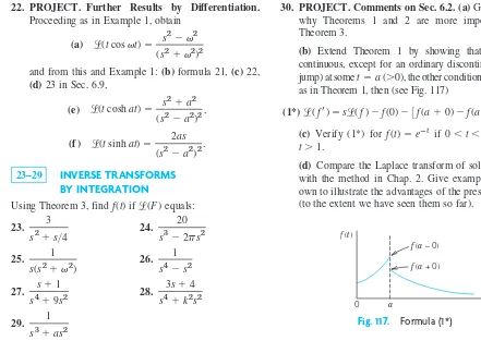
The unit step functionor Heaviside function is 0 for has a jump of size 1 at (where we can leave it undefined), and is 1 for in a formula:

(1) _u(ta)b (a_0).

0 if t_a

1 if t_a

t_a, t_a

t_a, u(t_a)

u

₍

t

a

₎

d_(ta)

u(t_a) f(t)

f(a – 0)

f(a + 0)

0 a t

Figure 118 shows the special case which has its jump at zero, and Fig. 119 the general case for an arbitrary positive a. (For Heaviside, see Sec. 6.1.)

The transform of follows directly from the defining integral in Sec. 6.1,

;

here the integration begins at because is 0 for Hence

(2) l_{u(ta)} e (s_0).

ⴚas s

t_a. u(t_a)

ta(₀₎

l_{u(ta)}

冮

ⴥ

0

eⴚst_{u(ta) dt}

冮

ⴥ

0

eⴚst

#

_{1 dt} eⴚst s `

ⴥ

t_a u(t_a)

u(t_a)

u(t), u(t)

t 1

0

u(t – a)

a t

1

0

Fig. 118. Unit step function u₍t₎ Fig. 119. Unit step function u₍ta₎

f(t)

(A) f(t) = 5 sin t (B) f(t)u(t – 2) (C) f(t – 2)u(t – 2) t

5

0

–5

t 5

0

–5

t 5

0

–5 +2 2 π +2

π 2π 2π 2π 2π

Fig. 120. Effects of the unit step function: (A) Given function. (B) Switching off and on. (C) Shift.

The unit step function is a typical “engineering function” made to measure for engineering applications, which often involve functions (mechanical or electrical driving forces) that are either “off ” or “on.” Multiplying functions with we can produce all sorts of effects. The simple basic idea is illustrated in Figs. 120 and 121. In Fig. 120 the given function is shown in (A). In (B) it is switched off between and (because when and is switched on beginning at In (C) it is shifted to the right by 2 units, say, for instance, by 2 sec, so that it begins 2 sec later in the same fashion as before. More generally we have the following.

Let for all negative t. Then with is shifted

(translated)to the right by the amount a.

Figure 121 shows the effect of many unit step functions, three of them in (A) and infinitely many in (B) when continued periodically to the right; this is the effect of a rectifier that clips off the negative half-waves of a sinuosidal voltage. CAUTION!Make sure that you fully understand these figures, in particular the difference between parts (B) and (C) of Fig. 120. Figure 120(C) will be applied next.

f(t) a₀ f(t_a)u(ta)

f(t)₀

t_2. t₂₎

u(t₂₎₀

t₂ t₀

Time Shifting (

t

_{-Shifting): Replacing}

t

_by

The first shifting theorem (“s-shifting”) in Sec. 6.1 concerned transforms

and The second shifting theorem will concern functions and Unit step functions are just tools, and the theorem will be needed to apply them in connection with any other functions.

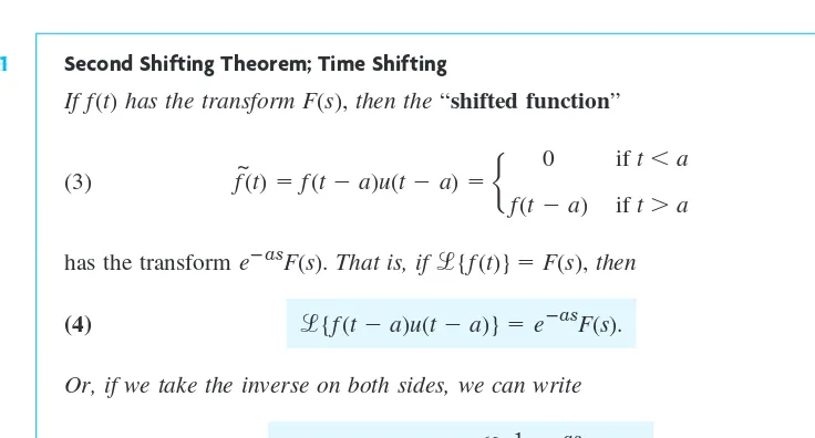
T H E O R E M 1 Second Shifting Theorem; Time Shifting

If has the transform then the“shifted function”

(3)

has the transform That is, if then

(4)

Or, if we take the inverse on both sides, we can write (4*)

Practically speaking, if we know we can obtain the transform of (3) by multiplying by In Fig. 120, the transform of 5 sin tis hence the shifted function 5 sin shown in Fig. 120(C) has the transform

P R O O F We prove Theorem 1. In (4), on the right, we use the definition of the Laplace transform, writing for t(to have tavailable later). Then, taking inside the integral, we have

Substituting , thus , in the integral (CAUTION, the lower limit changes!), we obtain

eⴚas_F(s)

冮

ⴥ

a

eⴚst_{f(ta) dt.}

dt_dt

t_ta

t_at

eⴚas_F(s)eⴚas

冮

ⴥ

0 eⴚst

f(t_{) d}t

冮

ⴥ

0

eⴚs(t_a) f(t_{) d}t_.

eⴚas

t

eⴚ2s_F(s)5eⴚ2s_>(s2_1).

(t_2)u(t2)

F(s)_5>(s2_1), eⴚas_.

F(s)

F(s),

f(t_a)u(ta) lⴚ1_{eⴚas_F(s)}.

l_{{f(ta)u(ta)}e}ⴚas_F(s).

l_{f(t)}F(s), eⴚas_F(s).

f~(t)_f(ta)u(ta)b

0 if t_a

f(t_{a) if ta} F(s),

f(t) f(t_a).

f(t) F(s_a)l_{eat_f(t)}.

F(s)l_{f(t)}

t

a

_in

f

₍

t

₎

SEC. 6.3 Unit Step Function (Heaviside Function). Second Shifting Theorem (t_{-Shifting) 219}

(A) k[u(t – 1) – 2u(t – 4) + u(t – 6)] (B) 4 sin ( πt)[u(t) – u(t – 2) + u(t – 4) – + ⋅⋅⋅]

t 2

0 4 6 8 4

k

–k ₁₀

1 _ 2 6

4

1 t

To make the right side into a Laplace transform, we must have an integral from 0 to , not from ato . But this is easy. We multiply the integrand by . Then for tfrom 0 to athe integrand is 0, and we can write, with as in (3),

(Do you now see why appears?) This integral is the left side of (4), the Laplace transform of in (3). This completes the proof.

E X A M P L E 1 Application of Theorem 1. Use of Unit Step Functions

Write the following function using unit step functions and find its transform.

(Fig. 122)

Solution. Step 1. In terms of unit step functions,

Indeed, gives for , and so on.

Step 2. To apply Theorem 1, we must write each term in in the form . Thus, remains as it is and gives the transform . Then

Together,

If the conversion of to is inconvenient, replace it by

(4**) .

(4**) follows from (4) by writing , hence and then again writing ffor g. Thus,

as before. Similarly for . Finally, by (4**),

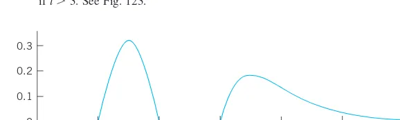
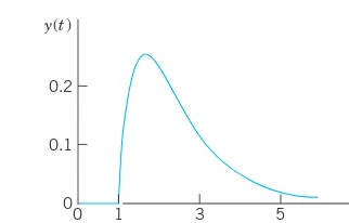
E X A M P L E 2 Application of Both Shifting Theorems. Inverse Transform

Find the inverse transform of

Solution. Without the exponential functions in the numerator the three terms of would have the inverses , and because has the inverse t, so that has the inverse by the first shifting theorem in Sec. 6.1. Hence by the second shifting theorem (t-shifting),

Now and so that the first and second terms cancel each other

when Hence we obtain if if 0 if and

if t3.See Fig. 123. _䊏

(t3)eⴚ2(tⴚ3)

2t3, 1t2,

0t1, (sin pt)>p

f(t)0

t2.

sin (pt2p)sin pt, sin (ptp) sin pt

f(t)1

p sin (p(t1)) u(t1)

1

p sin (p(t2)) u(t2)(t3)eⴚ 2(t3)

u(t_3).

teⴚ2t

1>(s2)2

1>s2

teⴚ2t

(sin pt)>p, (sin pt)>p

F(s)

F(s) e

ⴚs

s2p2

e

ⴚ2s

s2p2

e

ⴚ3s

(s₂₎2.

f(t)

SEC. 6.3 Unit Step Function (Heaviside Function). Second Shifting Theorem (t_{-Shifting) 221}

2

1

0

–1

␲ 2␲

1 4␲ t

f(t)

Fig. 122. ƒ(t_{) in Example 1}

0.3

0.2

0.1

1

0 2 3 4 5 6

0

t

Fig. 123. ƒ(t_{) in Example 2}

v(t)

t a

0 0

V₀

b a b t

v(t)

R C

i(t)

V₀/R

Fig. 124. RC_{-circuit, electromotive force} v₍t_{), and current in Example 3} E X A M P L E 3 Response of an RC_{-Circuit to a Single Rectangular Wave}

Find the current in the RC-circuit in Fig. 124 if a single rectangular wave with voltage is applied. The circuit is assumed to be quiescent before the wave is applied.

Solution. The input is Hence the circuit is modeled by the integro-differential equation (see Sec. 2.9 and Fig. 124)

Ri(t)q(t)

C

_Ri(t)1

C

冮

t

0

i(t) dtv(t)_{V03u(ta)u(tb)4.}

V03u(ta) u(tb)4.

V0

Using Theorem 3 in Sec. 6.2 and formula (1) in this section, we obtain the subsidiary equation

Solving this equation algebraically for we get

where and

the last expression being obtained from Table 6.1 in Sec. 6.1. Hence Theorem 1 yields the solution (Fig. 124)

that is, and

where and

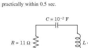
E X A M P L E 4 Response of an RLC_{-Circuit to a Sinusoidal Input Acting Over a Time Interval}

Find the response (the current) of the RLC-circuit in Fig. 125, where E(t) is sinusoidal, acting for a short time interval only, say,

if and if

and current and charge are initially zero.

Solution. The electromotive force can be represented by Hence the model for the current in the circuit is the integro-differential equation (see Sec. 2.9)

From Theorems 2 and 3 in Sec. 6.2 we obtain the subsidiary equation for

Solving it algebraically and noting that we obtain

For the first term in the parentheses times the factor in front of them we use the partial fraction expansion

Now determine A, B, D, Kby your favorite method or by a CAS or as follows. Multiplication by the common denominator gives

400,000s_A(s100)(s2₄₀₀2₎

B(s_10)(s2₄₀₀2₎₍

Ds_{K)(s10)(s100).}

400,000s

(s10)(s100)(s24002₎

A

s10

B

s100

DsK

s24002.

(Á)

l(s) 1000

#₄₀₀

(s10)(s100)a

s

s24002

seⴚ2ps

s24002b.

s2110s1000(s10)(s100), 0.1sI_11I100 I

s

100#400s

s24002a

1

s

eⴚ2ps

s b.

I(s)l(i)

i(0)_{0, ir(0)0.}

0.1ir_11i100

冮

t

0

i(t) dt_{(100 sin 400t)(1u(t2}p)).

i(t)

(100 sin 400t)(1u(t2p)).

E(t)

t2p

E(t)0

0t2p

E(t)100 sin 400t

䊏

K2V0eb>(RC)>R.

K1V0ea>(RC)>R

i(t)c

K1eⴚt>

(RC) _if

atb

(K1K2)eⴚt>

(RC) _if

ab

i(t)_{0 if ta,}

i(t)lⴚ1₍

I)lⴚ1_{

eⴚas_F(s)}lⴚ1_{

eⴚbs_F(s)}V0

R 3e

ⴚ(tⴚa)>(RC)

u(ta)eⴚ(tⴚb)>(RC)

u(tb)4;

lⴚ1

(F)V0

Re

ⴚt>(RC)

,

F(s) V0IR

s1>(RC)

I(s)F(s)(eⴚas_eⴚbs₎

I(s),

RI(s)I(s)

sC

V0

s 3e

We set and and then equate the sums of the and terms to zero, obtaining (all values rounded)

Since we thus obtain for the first term in

From Table 6.1 in Sec. 6.1 we see that its inverse is

This is the current when It agrees for with that in Example 1 of Sec. 2.9 (except for notation), which concerned the same RLC-circuit. Its graph in Fig. 63 in Sec. 2.9 shows that the exponential terms decrease very rapidly. Note that the present amount of work was substantially less.

The second term of Idiffers from the first term by the factor Since

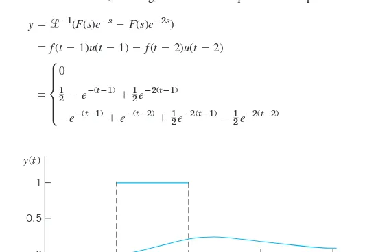
and the second shifting theorem (Theorem 1) gives the inverse if and for it gives

Hence in the cosine and sine terms cancel, and the current for is

It goes to zero very rapidly, practically within 0.5 sec. _䊏

i(t) 0.2776(eⴚ10t_eⴚ10(tⴚ2p)_)2.6144(

eⴚ100t_eⴚ100(tⴚ2p)_).

t2p

i(t)

i2(t) 0.2776eⴚ10(tⴚ2

p)_2.6144

eⴚ100(tⴚ2p)_{2.3368 cos 400}

t_{0.6467 sin 400t.} 2p

0t2p,

i2(t)0

sin 400(t2p)sin 400t,

cos 400(t2p)cos 400t eⴚ2ps_.

I1

0t2p

0t2p.

i(t)

i1(t) 0.2776eⴚ10t2.6144eⴚ100t2.3368 cos 400t0.6467 sin 400t.

I1

0.2776

s₁₀

2.6144

s₁₀₀

2.3368s

s2₄₀₀2

0.6467#400

s2₄₀₀2 .

I_I1I2

I1

K_258.660.6467#_400,

(s2-terms) 0100A10B110DK, K258.66. (s3-terms) 0ABD, D 2.3368 (s 100) 40,000,000 90(1002₄₀₀2₎

B, B2.6144 (s 10) 4,000,00090(102₄₀₀2₎

A, A 0.27760

s2

s3

₁₀₀

s 10

SEC. 6.3 Unit Step Function (Heaviside Function). Second Shifting Theorem (t_{-Shifting) 223}

E(t)

R = 11 Ω L = 0.1 H C = 10–2 _F

Fig. 125. RLC_{-circuit in Example 4}

1. Report on Shifting Theorems. Explain and compare the different roles of the two shifting theorems, using your own formulations and simple examples. Give no proofs.

2–11 SECOND SHIFTING THEOREM, UNIT STEP FUNCTION

Sketch or graph the given function, which is assumed to be zero outside the given interval. Represent it, using unit step functions. Find its transform. Show the details of your work.

2. 3.

4. _{cos 4t (0t}p₎ 5. et(0_tp_>2) t_{2 (t2)}

t (0_t2)

6. 7. 8. 9. 10. 11.

12–17 INVERSE TRANSFORMS BY THE 2ND SHIFTING THEOREM

Find and sketch or graph if equals

12. 13. 14. 15. 16.

17. (1eⴚ2p(s1)₎₍

s1)>((s1)2₁₎ 2(eⴚs_eⴚ3s₎

>(s2₄₎

eⴚ3s_>s4 4(eⴚ2s_2eⴚ5s_)>s

6(1_eⴚps_)>(s2₉₎ eⴚ3s

>(s₁₎3

l( f ) f(t)

sin t (p_>2tp) sinh t (0t2)

t2 (t3₂₎

t2 (1_t2)

eⴚpt_(2t4)

18–27 IVPs, SOME WITH DISCONTINUOUS INPUT

Using the Laplace transform and showing the details, solve

18.

28–40 MODELS OF ELECTRIC CIRCUITS

28–30 RL_-CIRCUIT

Using the Laplace transform and showing the details, find the current in the circuit in Fig. 126, assuming and:

31. Discharge in RC-circuit. Using the Laplace transform, find the charge q(t) on the capacitor of capacitance C in Fig. 127 if the capacitor is charged so that its potential is and the switch is closed at

32–34 RC_-CIRCUIT

Using the Laplace transform and showing the details, find the current i(t) in the circuit in Fig. 128 with and where the current at is assumed to be zero, and:

Fig. 126. Problems 28–30

v(t)

C R

Fig. 128. Problems 32–34

v(t)

C L

Fig. 129. Problems 35–37

C R

Fig. 127. Problem 31

35–37 LC_-CIRCUIT

Using the Laplace transform and showing the details, find the current in the circuit in Fig. 129, assuming zero initial current and charge on the capacitor and:

35. if

Using the Laplace transform and showing the details, find the current i(t) in the circuit in Fig. 130, assuming zero initial current and charge and:

SEC. 6.4 Short Impulses. Dirac’s Delta Function. Partial Fractions 225

6.4

Short Impulses. Dirac’s Delta Function.

Partial Fractions

An airplane making a “hard” landing, a mechanical system being hit by a hammerblow, a ship being hit by a single high wave, a tennis ball being hit by a racket, and many other similar examples appear in everyday life. They are phenomena of an impulsive nature where actions of forces—mechanical, electrical, etc.—are applied over short intervals of time.

We can model such phenomena and problems by “Dirac’s delta function,” and solve them very effecively by the Laplace transform.

To model situations of that type, we consider the function

(1) (Fig. 132)

(and later its limit as ). This function represents, for instance, a force of magnitude acting from to where k is positive and small. In mechanics, the integral of a force acting over a time interval is called the impulse of the force; similarly for electromotive forces E(t) acting on circuits. Since the blue rectangle in Fig. 132 has area 1, the impulse of in (1) is

(2) Ik

冮

ⴥ

0

fk(ta) dt

冮

a_k

a 1 k dt1. fk

a_tak t_ak,

t_a 1>k

k:0

fk(ta)b

1>k if a_tak 0 otherwise R

C

L

v(t)

Fig. 130. Problems 38–40

10

0

–20 –10

10 12 8

6 t

20 30

4 2

Fig. 131. Current in Problem 40 39. if

and 0 if t2 0t2

v(t)_{1 kV}

C_{0.5 F,}

L_{1 H,}

R_{2 , 40.}

if 0t2pand 0 if t2p

v_{255 sin t V}

C_{0.1 F,}

L_{1 H,}

R_{2 ,}

t a

1/k

Area = 1

a + k

To find out what will happen if kbecomes smaller and smaller, we take the limit of

as This limit is denoted by that is,

is called the Dirac delta function2or the unit impulse function.

is not a function in the ordinary sense as used in calculus, but a so-called generalized function.2To see this, we note that the impulse of is 1, so that from (1) and (2) by taking the limit as we obtain

(3)

but from calculus we know that a function which is everywhere 0 except at a single point must have the integral equal to 0. Nevertheless, in impulse problems, it is convenient to operate on as though it were an ordinary function. In particular, for a continuous function g(t) one uses the property [often called the sifting property of not to be confused with shifting]

(4)

which is plausible by (2).

To obtain the Laplace transform of we write

and take the transform [see (2)]

We now take the limit as By l’Hôpital’s rule the quotient on the right has the limit 1 (differentiate the numerator and the denominator separately with respect to k, obtaining and s, respectively, and use as ). Hence the right side has the limit This suggests defining the transform of by this limit, that is,

(5)

The unit step and unit impulse functions can now be used on the right side of ODEs modeling mechanical or electrical systems, as we illustrate next.

l_{d_(ta)}eⴚas_.

d_(ta) eⴚas_.

k:0 seⴚks_>s

:1

seⴚks

k:0.

l_{fk(ta)} 1 ks3e

ⴚas_eⴚ(ak)s_4eⴚas1e ⴚks

ks .

fk(ta) 1

k3u(ta)u(t(ak))4

d_(ta),

冮

ⴥ

0

g(t)d_{(ta) dtg(a)}

d(t_a),

d(t_a)

d(t_a)b

_{if ta}

0 otherwise and

冮

ⴥ

0

d(t_{a) dt1,} k:0

fk Ik

d(t_a)

d(t_a)

d(t_{a) lim} k_:0 fk(t

_a).

d(t_a), k:0 (k0).

fk

2_{PAUL DIRAC (1902–1984), English physicist, was awarded the Nobel Prize [jointly with the Austrian}

ERWIN SCHRÖDINGER (1887–1961)] in 1933 for his work in quantum mechanics.

E X A M P L E 1 Mass–Spring System Under a Square Wave

Determine the response of the damped mass–spring system (see Sec. 2.8) under a square wave, modeled by (see Fig. 133)

Solution. From (1) and (2) in Sec. 6.2 and (2) and (4) in this section we obtain the subsidiary equation

Using the notation F(s) and partial fractions, we obtain

From Table 6.1 in Sec. 6.1, we see that the inverse is

Therefore, by Theorem 1 in Sec. 6.3 (t-shifting) we obtain the square-wave response shown in Fig. 133,

䊏

d

0 (0_t1)

1 2eⴚ

(tⴚ1)1 2eⴚ

2(tⴚ1)

(1_{t2) e}ⴚ(tⴚ1)

eⴚ(tⴚ2)1

2eⴚ 2(tⴚ1)1

2eⴚ 2(tⴚ2)

(t_{2). f(t1)u(t1)f(t2)u(t2)}

ylⴚ1₍

F(s)eⴚs_F(s)eⴚ2s₎

f(t)lⴚ1₍

F)1

2eⴚt 1 2eⴚ

2t_.

F(s) 1

s(s2_3s2)

1

s(s_1)(s2)

1 2

s

1

s₁

1 2

s₂.

s2_Y3sY2Y1

s (e

ⴚseⴚ2s_).

Solution Y(s) 1

s(s23s2) (eⴚ

s_eⴚ2s_).

ys₃yr₂yr(t)u(t₁₎u(t_2), y(0)_0, yr(0)_0.

SEC. 6.4 Short Impulses. Dirac’s Delta Function. Partial Fractions 227

t y(t)

0.5

0

1 0

1

2 3 4

Fig. 133. Square wave and response in Example 1

E X A M P L E 2 Hammerblow Response of a Mass–Spring System

Find the response of the system in Example 1 with the square wave replaced by a unit impulse at time

Solution. We now have the ODE and the subsidiary equation

Solving algebraically gives

By Theorem 1 the inverse is

y(t)lⴚ1

(Y)c 0 if 0 t₁

eⴚ(tⴚ1)

eⴚ2(tⴚ1)

if t_1.

Y(s) e

ⴚs

(s₁₎₍s₂₎ a 1

s₁

1

s₂be

ⴚs_.

ys_3yr2yd_{(t1), and (s}2₃

s_2)Yeⴚs_.

y(t) is shown in Fig. 134. Can you imagine how Fig. 133 approaches Fig. 134 as the wave becomes shorter and shorter, the area of the rectangle remaining 1? 䊏

t y(t)

0.1

0 0.2

1

0 3 5

Fig. 134. Response to a hammerblow in Example 2

v(t) = ? ␦(t)

R

A B

L

C

40

0 80

–80 –40

0.25 0.3 0.2

0.15

0.05 t

v

0.1

Network Voltage on the capacitor

Fig. 135. Network and output voltage in Example 3 E X A M P L E 3 Four-Terminal RLC_-Network

Find the output voltage response in Fig. 135 if the input is (a unit impulse at time ), and current and charge are zero at time

Solution. To understand what is going on, note that the network is an RLC-circuit to which two wires at A

and Bare attached for recording the voltage v(t) on the capacitor. Recalling from Sec. 2.9 that current i(t) and charge q(t) are related by we obtain the model

From (1) and (2) in Sec. 6.2 and (5) in this section we obtain the subsidiary equation for

By the first shifting theorem in Sec. 6.1 we obtain from Qdamped oscillations for qand v; rounding we get (Fig. 135)

䊏

qlⴚ1_(Q) 1

99.50e

ⴚ10t _{sin 99.50t}

and vq

C

_100.5eⴚ10t_{sin 99.50t.}

9900⬇99.502_,

(s2_{20s10,000)Q1.}

Solution Q 1

(s₁₀₎2₉₉₀₀.

Q(s)l(q)

LirRi

q

C

LqsRqr

q

C

qs20qr10,000qd(t).

iqrdq>dt,

t0.

t0

d(t)

C10ⴚ4 _F,

L1 H,

R20 ,

More on Partial Fractions

We have seen that the solution Y of a subsidiary equation usually appears as a quotient of polynomials so that a partial fraction representation leads to a sum of expressions whose inverses we can obtain from a table, aided by the first shifting theorem (Sec. 6.1). These representations are sometimes called Heaviside expansions.

An unrepeated factor in G(s) requires a single partial fraction

See Examples 1 and 2. Repeated real factors , etc., require partial fractions

etc.,

The inverses are etc.

Unrepeated complex factors , require a partial

fraction For an application, see Example 4 in Sec. 6.3.

A further one is the following.

E X A M P L E 4 Unrepeated Complex Factors. Damped Forced Vibrations

Solve the initial value problem for a damped mass–spring system acted upon by a sinusoidal force for some time interval (Fig. 136),

Solution. From Table 6.1, (1), (2) in Sec. 6.2, and the second shifting theorem in Sec. 6.3, we obtain the subsidiary equation

We collect the Y-terms, take to the right, and solve,

(6)

For the last fraction we get from Table 6.1 and the first shifting theorem

(7)

In the first fraction in (6) we have unrepeated complex roots, hence a partial fraction representation

Multiplication by the common denominator gives

We determine A, B, M, N. Equating the coefficients of each power of son both sides gives the four equations

(a) (b)

(c) (d)

We can solve this, for instance, obtaining from (a), then from (c), then from (b), and finally from (d). Hence and the first fraction in (6) has the representation

(8) 2s2

s2₄

2(s

₁₎₆₂

(s₁₎2₁ . Inverse transform:

_{2 cos 2tsin 2te}ⴚt_{(2 cos t4 sin t).}

N_6,

M_2,

B 2,

A 2,

A 2

N 3A

A_B

M A

3s0

4: 20₂B₄N.

3s4: 0₂A₂B₄M

3s2

4: 0₂ABN

3s3

4: 0AM

20₍AsB)(s2_2s2)(MsN)(s2_4).

20 (s2_4)(s2_2s2)

AsB

s2₄

MsN

s2_2s2.

lⴚ1

b s14

(s₁₎2₁r

_eⴚt_{(cos t4 sin t).}

Y 20

(s24)(s22s2)

20e

ⴚps

(s24)(s22s2)

s3

s22s2.

s₅₂ s₃

(s2_2s2)Y,

(s2Ys5)2(sY1)2Y10 2

s24 (1

eⴚps_).

ys2yr2yr(t), r(t)10 sin 2t if 0tp and 0 if tp; y(0)1, yr(0) 5.

(As_B)>3(sa)2b24.

aaib aa_ib,

(s_a)(sa), (1

2A3t2A2tA1)eat, (A2tA1)eat,

A2 (s_a)2

A1

sa, A3 (s_a)3

A2 (s_a)2

A1 sa, (s_a)3 (s_a)2_,

A>(s_a). sa