ELECTRICAL ENGINEERING
Optimal location of STATCOM using chemical
reaction optimization for reactive power dispatch
problem
Susanta Dutta
a, Provas Kumar Roy
b,*, Debashis Nandi
ca
Department of Electrical Engineering, Dr. B.C. Roy Engineering College, Durgapur, West Bengal, India
b
Department of Electrical Engineering, Jalpaiguri Government Engineering College, Jalpaiguri, West Bengal, India
c
Department of Information Technology, National Institute of Technology, Durgapur, West Bengal, India
Received 10 October 2014; revised 1 April 2015; accepted 26 April 2015 Available online 12 June 2015
KEYWORDS
Flexible AC transmission system;
Static synchronous compensator (STATCOM); Optimal reactive power dispatch (ORPD); Chemical reaction optimization (CRO); Transmission loss
Abstract Optimal reactive power dispatch (ORPD) problem has a significant influence on optimal operation of power systems. However, getting optimal solution of ORPD problem is a strenuous task for the researchers. The inclusion of flexible AC transmission system (FACTS) devices in the power system network for solving ORPD problem adds to its complexity. This paper presents the application of chemical reaction optimization (CRO) for optimal allocation of a static syn-chronous compensator (STATCOM) to minimize the transmission loss, improve the voltage profile and voltage stability in a power system. The proposed approach is carried out on IEEE 30-bus and IEEE 57-bus test systems and the simulation results are presented to validate the effectiveness of the proposed method. The results show that the proposed approach can converge to the optimum solu-tion and obtains better solusolu-tions as compared to other methods reported in the literature. 2015 Faculty of Engineering, Ain Shams University. Production and hosting by Elsevier B.V. This is an open access article under the CC BY-NC-ND license (http://creativecommons.org/licenses/by-nc-nd/4.0/).
1. Introduction
The electric power grid is the largest man-made machine in the world. It consists of synchronous generators, transformers,
transmission lines, switches and relays, active/reactive compo-nents, and loads. Power system networks are complex systems that are nonlinear, non-stationary, and prone to disturbances and faults. Reinforcement of a power system can be accom-plished by improving the voltage profile, increasing the trans-mission capacity and others. Nevertheless, some of these solutions may require considerable investment that could be difficult to recover. FACTS devices are an alternate solution to address some of those problems[1,2].
Optimal reactive power dispatch (ORPD) is an important tool for power system operators for both planning and reliable operation in the present day power systems. The important aspect of ORPD is to determine the optimal settings of control variables for minimizing transmission loss, improve the * Corresponding author at: Jalpaiguri Government Engineering
College, Jalpaiguri, 735102, West Bengal, India. Tel.: +91 9474521395; fax: +91 3561 256143.
E-mail address:[email protected](P.K. Roy). Peer review under responsibility of Ain Shams University.
Production and hosting by Elsevier
Ain Shams University
Ain Shams Engineering Journal
www.elsevier.com/locate/asej www.sciencedirect.com
http://dx.doi.org/10.1016/j.asej.2015.04.013
voltage profile and voltage stability, while satisfying various equality and inequality constraints. The ORPD problem is in general non-convex and non-linear and exists many local minima.
Over the last two decades, many researchers performed a lot of researches on ORPD. Various optimization techniques are evolved to solve ORPD problem. These algorithms are generally divided into two categories, namely, classical mathe-matical optimization algorithms and intelligent optimization algorithms. The classical algorithms are starting from an initial point, continuously improve the current solution through a certain orbit, and ultimately converging to the optimal solu-tion. These algorithms include linear programming (LP) [3]
quadratic programming (QP) [4], non-linear programming (NLP)[5]and mixed integer linear programming (MILP)[6], and benders decomposition[7]. Though, some of these tech-niques, have a good convergence but most of them suffer from local optimality. Since ORPD is multimodal and non-linear optimization problem and severely depends on the initial guess, the classical techniques are unable to produce global optimal solution. To overcome this deficiency, various intelli-gent optimization algorithms known as heuristic techniques are applied to solve ORPD problem. Some of the well popular optimization techniques are evolutionary programming (EP)
[8], genetic algorithm (GA) [9,10], simulated annealing (SA)
[11,12], tabu search (TS) [13,14], differential evolution (DE)
[15,16], particle swarm optimization (PSO)[17,18] and artifi-cial bee colony (ABC)[19], etc. Recently, a harmony search algorithm (HSA) was developed by Sirjani et al.[20]for simul-taneous minimization of total cost, the voltage stability index, voltage profile and power loss of IEEE 57-bus test system using shunt capacitors, SVC and static synchronous compen-sators (STATCOM). Saravanan et al. presented PSO[21]to find optimal settings and location TCSC, SVC and UPFC devices for improving system load ability with minimum cost of installation.
The literature survey shows that most of the population based techniques successfully solved optimal located FACTS based ORPD problem. However, the slow convergence toward the optimal solution is the main concern for most of these heuristics algorithms. Furthermore, these techniques often produce the local optimal solution rather than global optimal solution.
In this article, a recently developed heuristic algorithm named chemical reaction optimization (CRO) algorithm based on the different chemical reactions on the molecular structure of molecules, introduced by Lam et al. in 2010 is used to find the optimal location of STATCOM device for solving ORPD problem. The effectiveness of the proposed CRO algorithm is demonstrated by implementing it in two standard systems namely IEEE 30-bus and IEEE 57-bus systems and its perfor-mance is compared with PSO, DE and other optimization techniques recently published in the literature.
The remaining sections of this paper are organized as fol-lows: Section2describes the problem formulation of ORPD problem. Section 3briefly describes the CRO technique and the different steps of the proposed CRO approach. Section4
discusses the computational procedure and analyzes the DE, PSO and CRO results when applied to case studies of FACTS based ORPD problem. Lastly, Section5outlines the conclusions.
2. Mathematical problem formulation
2.1. Static model and mathematical analysis of static synchronous compensator
Although, there are several FACTS devices for controlling power flow [22]and voltage profile in power system, for this study, only STATCOM device is considered to minimize the transmission loss, improve the voltage profile and voltage sta-bility of power system network. Static model of this FACTS device is as described below.
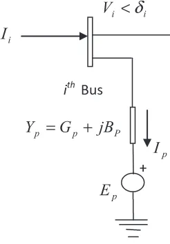
Static synchronous compensator (STATCOM) is connected in parallel with the specific bus of a power system. The primary goal of STATCOM is to enhance the reactive power compen-sation which adjusts the reactive power and voltage magnitude of power system network. It consists of three basic compo-nents, namely, transformer, voltage source converter (VSC) and capacitor. The STATCOM is modeled as a controllable voltage source (Ep) in series with an impedance[23]. The real
part of this impedance represents the cupper losses of the cou-pling transformer and converter, while the imaginary part of this impedance represents the leakage reactance of the cou-pling transformer. STATCOM absorbs requisite amount of reactive power from the grid to keep the bus voltage within reasonable range for all power system loading.Fig. 1 shows the circuit model of a STATCOM connected to the ith bus of a power system. The injected active and reactive power flow equation of theith bus are given below:
Pi¼GpjVij2 jVijjEpjjYpjcosðdidphpÞ
þX
N
j¼1
jVijjVjjjYijjcosðdidjhijÞ ð1Þ
Qi¼ BpjVij
2
jVijjEpjjYpjsinðdidphpÞ
þX
N
j¼1
jVijjVjjjYijjsinðdidjhijÞ ð2Þ
The implementation of STATCOM in transmission system introduces two state variables (|Ep| anddp); however, |Vi| is
known for STATCOM connected bus. It may be assumed that
the power consumed by the STATCOM source is zero in
the STATCOM;Gp,Bp are the conductance and susceptance,
respectively, of the STATCOM;hijis the admittance angle of transmission line connected between theith bus andjth bus, respectively; dp is the voltage source angle of the STATCOM; Ep is the voltage sources of STATCOM
converters.
2.2. Objective function
The conventional formulation of ORPD problem determines the optimal setting of control variables such as generator ter-minal voltages, transformers tap setting, reactive power of shunt compensators, controllable voltage source of STATCOM and its phase angle to minimize the transmission loss while satisfying the operational constraints. However, in order operate the power system in reliable and secure mode, the voltage profile and voltage stability index of the power sys-tem are also considered as the objective functions in this study.
2.2.1. Minimization of total real power loss
The objective of transmission loss minimization may be expressed by
wheref1ðx;yÞ is the transmission loss minimization objective function;Ploss is the total active power loss;Gkis the
conduc-tance of thekth line connected between themith andjth buses;
Vi,Vjare the voltage of theith andjth buses, respectively;di,dj
are the phase angle of theith andjth bus voltages.xis the vec-tor of dependent variable consisting of load voltages (Vl1;. . .VlNL), generators’ reactive powers (Qg1;. . .;QgNG),
Therefore, the independent and dependent vectors may be expressed as
where NG;NL are the number of generator and load buses;
NTL;NT;NCare the number of transmission lines, regulating transformers and shunt compensators, respectively.
2.2.2. Minimization of voltage deviation
Since bus voltage is one of the most important security and ser-vice quality indexes of the power system, the minimization of deviations of voltages from desired values is considered as another objective in this study. The objective function of volt-age profile improvement, i.e. voltvolt-age deviation minimization at load buses, may be expressed as:
f2ðx;yÞ ¼min voltage at theith load bus, usually set to 1.0 p.u.
2.2.3. Minimization of L-index
It is very important to maintain constantly acceptable bus volt-age at each bus under normal operating conditions. However, when the system is subjected to a disturbance, the system con-figuration is changed. The non-optimized control variables may lead to progressive and uncontrollable drop in voltage resulting in an eventual widespread voltage collapse. In this work, voltage stability enhancement is achieved through min-imizing the voltage stability indicator L-index. The indicator values vary in the range between 0 and 1.
The L-index of a power system is briefly discussed below: For a multi-node system, the relation among voltage and current of load and generator buses may be expressed as follows:
By matrix inversion, the above equation may be rearranged as follows:
The sub-matrixFlgmay be expressed as under:
Flg¼ ½yll
1
½ylg ð11Þ
The voltage stability index of thejth bus may be expressed by
Lj¼ 1
whereVg;Vlare the vectors of the bus voltage of the generator
and load buses, respectively;Ig;Il are the vectors of the bus
currents of the generator and load buses, respectively. Zll,
Flg,Kgl,Yggare the sub-matrices obtained by partial inversion
of the admittance matrix,Ng;Nl are the number of generator
and load buses, respectively.
To move the system far away from the voltage collapse point, the voltage stability index needs to minimize. The global L-index indicator of the power system is expressed as follows:
Lmax¼maxðL1;L2;. . .;LNlÞ ð13Þ
Therefore, to enhance the voltage stability and to move the system far from the voltage collapse margin, the objective function may be represented as follows:
2.2.4. Constraints
The ORPD incorporating STATCOM is subjected to the fol-lowing constraints:
where pgi;pli are the active power generation and demand,
respectively, of theith bus;qgi;qliare the reactive power
gener-ation and demand, respectively, of theith bus;gij;bijare the
conductance and susceptance, respectively, of the line con-nected between themith bus and jth bus and NB is number of buses.
gi ;vmaxgi are the voltage operating limits of theith
gen-erator bus;pmin
gi ;p
max
gi are the active power generation limits of
theith bus;qmin
gi ;qmaxgi are the reactive power generation limits
of theith bus;vmin
li ;v
max
li are the voltage limits of theith load
bus;sli;smaxli are the apparent power flow and maximum
appar-ent power flow limit of theith branch;tmin
i ;t
max
i are the tap
set-ting limits of theith regulating transformer;qmin
ci ;qmaxci are the
reactive power injection limits of theith shunt compensator;
dmax
pi ;
dmin
pi are the phase angle limits of the ith STATCOM;
Emaxp
i ;E min
pi are the voltage limits of the ith STATCOM;
NG;NL;NTL;NT;NCare the number of generator bus, load bus, transmission line, regulating transformer and shunt com-pensator; respectively.
3. Chemical reaction optimization
Chemical reaction optimization (CRO) was introduced by Lam and Li in the year 2010. It is a new optimization tech-nique based on the various chemical reactions occur among the molecules. A molecule consists of several atoms and is characterized by the atom type, bond length and torsion.
Any change in the atom type makes the molecules different from others. Each molecule has two kinds of energies PE (potential energy) and KE (kinetic energy). PE represents the objective function of a molecule while the KE of a molecule represents its ability of escaping from a local minimum.
During the CRO[24–26]process, the following four types of elementary reactions are likely to happen. These are on-wall ineffective collision, decomposition, inter-molecular inef-fective collision and synthesis. These reactions can be catego-rized into single molecular reactions and multiple molecular reactions. The on-wall ineffective collision and decomposition reactions are single molecular reactions, while the inter-molecular ineffective collision and synthesis reactions are of the latter category.
(1) On-wall ineffective collision
In this reaction process each molecule hits the wall of the container and generates a new molecule whose molecular structure is closed to the original one. Since, the On-wall inef-fective collision is not so severe, the resultant molecular struc-ture is not too different from the original one. A molecule ‘ms’ collides into the wall is allowed to change to another molecule ‘ms1’, if the constraint described below is satisfied.
PEmsþKEmsPPEms1 ð23Þ
(2) Decomposition
A single compound breaks down into two or more mole-cules in the decomposition process. In this reaction, the newly formed molecules are far away from the original molecule. As compared with on-wall ineffective collision, the generated molecules have greater change in the potential energy than the original ones. The moleculem, hits a wall of the container and participate in decomposition reaction, to generate two moleculesms1 andms2 if the inequality constraint(24)holds,
KEmsþPEms
PPEms1þPEms2 ð24Þ (3) Intermolecular ineffective collision
This chemical reaction takes place when two different mole-cules react among themselves, forming two different molemole-cules. However, in this reaction, the molecular structures of the newly generated molecules are closed to the original molecules. Therefore in this collision, the molecules react much less vigor-ously than decomposition collusion. When two molecules, ‘m1’ and ‘m2’, collide with each other, they may form to two new molecules,m1
1and ‘m21’, if the following inequality holds:
KEms1þPEms1þKEms2þPEms2 PPEms01þPEms02 ð25Þ (4) Synthesis
The synthesis reaction is opposite to the decomposition reaction. In this reaction two or more reactants combine together to form an entirely different new molecule. Synthesis collision allows the molecular structure to change in a larger extent. The two moleculesm1
1and ‘m21’ collide with each other and form a new moleculemif the following condi-tion is satisfied.
KEms1þPEms1þKEms2þPEms2PEms01 ¼KEms01: ð27Þ The various steps for implementing the CRO algorithm can be summarized as follows:
Step 1: The various input parameters of the CRO algo-rithm are initialized. The molecular structures of the molecules are generated randomly. The molecu-lar structures of the molecules represent various feasible solution vectors.
Step 2: The value of the objective function of the individual feasible solution set represents the potential energy (PE) of the individual molecule. An initial kinetic energy (KE) is assigned to all the molecules. Step 3: Depending upon the PE values, sort the population
and in order to retain the best solutions intact, few best molecules are kept as elite molecules.
Step 4: To allow the algorithm to escape from a local min-imum, the on-wall ineffective collision operations are performed on non-elite molecules. In this pro-cess, one molecule ms is selected randomly from the population and one moleculems1is generated using mutation operation as described below
msi2;j¼msk1;jþF msm1;jmsn1;j
i¼1;2;. . .;NP
ð28Þ
msk1;j;ms1m;j andmsn1;jare thejth components of three different molecules chosen randomly from the current population.
If there is enough energy for the new molecule to be gener-ated, i.e. if criterion(29)is satisfied, replace the original mole-cule with the new one, and update the relevant KE using(30).
KEmsþPEmsPPEms1 ð29Þ
KEms1
¼randKEmsþPEmsPEms1
ð30Þ Step 5: For each decomposition operation, two molecules are selected from the population and two molecules are generated by performing the crossover opera-tion of DE. Afterward, they are tested against the synthesis criterion: KEms
þPEms
PPEms1þPEms0
1. If this criterion is satisfied by the selected mole-cules, replace the original molecules by the newly generated molecules and update the KE of the new molecules using(31) and (32).
KEms1 ¼rand ½KEmsþPEms ðPEms1 þPEms0
1Þ ð31Þ
KEms0
1 ¼ ð1randÞ ½KEmsþPEms
PEms1þPEms01 ð32Þ Step 6: To enhance the search space, the inter-molecular ineffective collision is applied on each molecule to update its molecular structure. The inter-molecular ineffective collision occurs when two molecules collide and then produce two new mole-cules. To perform this reaction, two moleculesms1 andms2 from the population are selected and two new molecules ms0
1 andms02 are generated by per-forming the crossover operation of DE. The origi-nal molecules ms1 and ms2 are replaced by the new moleculesms0
1 andms02 if the newly generated molecules have better fitness value (PE). The KE of the molecules ms1 andms2 are modified using
(33) and (34)
KEms0
1 ¼rand½PEms1þKEms1þPEms2
þKEms2 PEms01þPEms02 ð33Þ
KEms0
2 ¼ ð1randÞ ½PEms1þKEms1þPEms2 þKEms2 PEms01þPEms02 ð34Þ Step 7: Lastly, the molecules participate in synthesis colli-sion operation to update their molecular structure. Two moleculesms1 andms2 are selected randomly from the population set and one molecule ms0
1 is generated by performing the crossover operation. If the newly generated molecule gives better func-tion value (PE), the new molecule is included and the original molecules are excluded. The new mole-culems0
1updates its KE using(35)
KEms0
1 ¼rand ðKEms1þPEms1þKEms2
þPEms2PEms01Þ ð35Þ Step 8: The feasibility of each solution is checked by
satis-fying its operational constraints.
Step 9: Sort the solutions from best to worst and replace the worst solution by the best elite solutions.
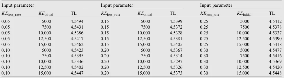
Table 1 Transmission loss for different input parameters of IEEE 30-bus system with STATCOM.
Input parameter Input parameter Input parameter
KEloss_rate KEinitial TL KEloss_rate KEinitial TL KEloss_rate KEinitial TL
0.05 5000 4.5494 0.15 5000 4.5399 0.25 5000 4.5412
0.05 7500 4.5431 0.15 7500 4.5372 0.25 7500 4.5378
0.05 10,000 4.5386 0.15 10,000 4.5328 0.25 10,000 4.5337
0.05 12,500 4.5417 0.15 12,500 4.5381 0.25 12,500 4.5390
0.05 15,000 4.5462 0.15 15,000 4.5405 0.25 15,000 4.5418
0.10 5000 4.5423 0.20 5000 4.5367 0.30 5000 4.5477
0.10 7500 4.5395 0.20 7500 4.5314 0.30 7500 4.5416
0.10 10,000 4.5346 0.20 10,000 4.5297 0.30 10,000 4.5369
0.10 12,500 4.5402 0.20 12,500 4.5326 0.30 12,500 4.5420
Step 10: The CRO algorithm is terminated when the termi-nation criterion is met. Otherwise go to Step 3.
4. Simulation results and discussions
In this paper, to assess the efficiency of the proposed CRO approach, two case studies (IEEE 30 bus and IEEE 57-bus sys-tems) of ORPD problems are used in the simulation study. All the programs are written in Matlab 7.0 and run on a PC with core i3 processor, 2.50 GHz, 4 GB RAM. The results of the ORPD problem obtained by CRO are compared with those obtained by DE, PSO and other techniques such as canonical GA (CGA) [27], the adaptive GA (AGA) [27], PSO with
adaptive inertia weight (PSO-w)[27], PSO with a constriction factor (PSO-cf) [27], the comprehensive learning particle swarm optimizer (CLPSO)[27], the standard version of PSO (SPSO)[27], local search DE with self-adapting control param-eters (L-SACP-DE)[27], seeker optimization algorithm (SOA)
[27], gravitational search algorithm (GSA)[28], teaching learn-ing based optimization (TLBO)[29], quasi-oppositional TLBO (QOTLBO) [29], strength pareto evolutionary algorithm (SPEA) [30], GA-1 [31]and GA-2 [32], multi-objective PSO (MOPSO-1)[33], DE-1[34], oppositional GSA (OGSA)[35], multi-objective PSO (MOPSO-2) [36], multi-objective improved PSO (MOIPSO) [36], multi-objective chaotic improved PSO (MOCIPSO) [36] available in the literature. Since the performance of any algorithm depends on its input parameters, they should be carefully chosen. After several runs, the following input parameters are found to be the best for the optimal performance of the DE and PSO algorithms.
DE: Scaling factor (F) = 0.7; crossover probability (CR) = 0.2.
PSO:C1=C2= 2.05;xmax= 0.9;xmin= 0.4.
For CRO, the average value of the transmission loss over 25 different trials of IEEE 30-bus system with STATCOM for different values of KEloss_rate and KEinitial is listed in
Table 1. It is clearly observed fromTable 1that the optimal settings of these input parameters for the optimal performance of the proposed CRO algorithm are as follows:
KEloss_rate= 0.2;KEinitialfor each molecule = 10,000.
4.1. IEEE 30-bus system
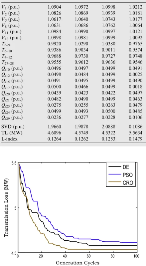
Firstly, the standard IEEE 30-bus system is used to evaluate the correctness and the relative performance of the proposed CRO method. This system consists of 6 generators, 4 regulat-ing transformers, 9 shunt compensators and 41 transmission Table 2 Comparison of simulation results obtained by different algorithms without STATCOM.
Control variables Real power loss minimization Voltage deviation minimization Voltage stability index minimization
PSO DE CRO PSO DE CRO PSO DE CRO
V1(p.u.) 1.0904 1.0972 1.0998 1.0212 1.0089 1.0092 1.0897 1.0867 1.0916
V2(p.u.) 1.0826 1.0869 1.0939 1.0181 1.0044 1.0050 1.0807 1.0811 1.0901
V5(p.u.) 1.0617 1.0640 1.0743 1.0177 1.0218 1.0195 1.0929 1.0919 1.0846
V8(p.u.) 1.0631 1.0686 1.0762 1.0064 1.0041 1.0031 1.0573 1.0568 1.0697
V11(p.u.) 1.0984 1.0990 1.0997 1.0121 1.0027 1.0390 1.0994 1.0991 1.0992
V13(p.u.) 1.0998 1.0981 1.0999 1.0092 1.0284 1.0144 1.0959 1.0988 1.0972
T6–9 0.9920 1.0290 1.0380 0.9765 1.0142 1.0551 0.9471 0.9396 0.9646
T6–10 0.9386 0.9034 0.9011 0.9574 0.9004 0.9001 0.9078 0.9011 0.9003
T4–12 0.9688 0.9730 0.9727 0.9748 1.0136 0.9937 0.9241 0.9361 0.9327
T27–28 0.9555 0.9612 0.9636 0.9546 0.9667 0.9663 0.9055 0.9001 0.9067
Qi10(p.u.) 0.0496 0.0497 0.0499 0.0491 0.0500 0.0499 0.0494 0.0468 0.0440
Qi12(p.u.) 0.0498 0.0484 0.0499 0.0025 0.0199 0.0424 0.0123 0.0466 0.0246
Qi15(p.u.) 0.0491 0.0495 0.0499 0.0490 0.0498 0.0500 0.0466 0.0499 0.0496
Qi17(p.u.) 0.0500 0.0466 0.0499 0.0018 0.0000 0.0000 0.0442 0.0492 0.0464
Qi20(p.u.) 0.0439 0.0423 0.0422 0.0497 0.0500 0.0500 0.0482 0.0499 0.0453
Qi21(p.u.) 0.0482 0.0490 0.0499 0.0463 0.0499 0.0500 0.0482 0.0485 0.0434
Qi23(p.u.) 0.0275 0.0255 0.0263 0.0479 0.0500 0.0500 0.0423 0.0499 0.0489
Qi24(p.u.) 0.0499 0.0493 0.0500 0.0485 0.0500 0.0500 0.0486 0.0498 0.0451
Qi29(p.u.) 0.0236 0.0277 0.0228 0.0106 0.0497 0.0258 0.0486 0.0498 0.0484
SVD (p.u.) 1.9660 1.9878 2.0888 0.1086 0.1029 0.0849 2.5601 2.6716 2.6503
TL (MW) 4.6096 4.5749 4.5322 5.5634 5.8973 5.8067 5.1374 5.1380 4.8617
L-index 0.1264 0.1262 0.1253 0.1479 0.1478 0.1490 0.1210 0.1198 0.1156
0 20 40 60 80 100
4.5 5 5.5
Generation Cycles
Transmission Loss (MW)
DE
PSO
CRO
lines. The generator and transmission-line data adopted from
[37]are illustrated inTables A1–A3. The maximum and mini-mum voltage limits at all the buses are taken as 1.10 p.u. and 0.95 p.u., respectively. The upper and lower tap settings limits of regulating transformers are taken as 1.10 p.u. and 0.9 p.u., respectively. The upper and lower voltage limits of
STATCOM are taken as 1.10 p.u. and 0.9 p.u., respectively. The limits of phase angle of STATCOM are taken as 2006d
p600. The resistance and reactance of equivalent
STATCOM converter is 0.01 p.u. and 0.1 p.u., respectively. The performance of the proposed CRO method is demon-strated by applying it in conventional ORPD problem (Case Table 3 Statistical comparison (50 trials) among various algorithms for IEEE 30-bus without STATCOM.
Real power loss minimization
Techniquesfi TLBO[29] QOTLBO[29] SPEA[30] GA-1[31] GA-2[32] PSO DE CRO
Best loss (MW) 4.5629 4.5594 5.1170 4.5800 4.5550 4.6096 4.5749 4.5322
Mean loss (MW) 4.5695 4.5601 NA NA NA 4.6503 4.6414 4.5413
Worst loss (MW) 4.5748 4.5617 NA NA NA 4.7831 4.7328 4.5476
Voltage deviation minimization
Techniquesfi TLBO[29] QOTLBO[29] MOPSO-1[33] DE-1[34] PSO DE CRO
Best VD 0.0913 0.0856 0.2424 0.0911 0.1086 0.1029 0.0849
Mean VD 0.0934 0.0872 NA NA 0.1132 0.1083 0.0863
Worst VD 0.0988 0.0907 NA NA 0.1254 0.1176 0.0898
Voltage stability index minimization
Techniquesfi TLBO[29] QOTLBO[29] SPEA[30] DE-1[34] PSO DE CRO
Best L index 0.1252 0.1242 0.1397 0.1246 0.1210 0.1198 0.1156
Mean L index 0.1254 0.1245 NA NA 0.1256 0.1221 0.1163
Worst L index 0.1258 0.1247 NA NA 0.1304 0.1283 0.1172
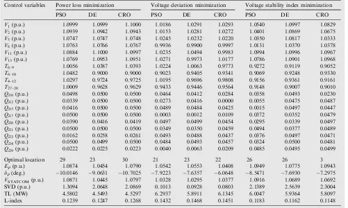
Table 4 Comparison of simulation results obtained by different algorithms with STATCOM.
Control variables Power loss minimization Voltage deviation minimization Voltage stability index minimization
PSO DE CRO PSO DE CRO PSO DE CRO
V1(p.u.) 1.0999 1.0999 1.1000 1.0186 1.0291 1.0293 1.0540 1.0997 1.0829
V2(p.u.) 1.0939 1.0942 1.0943 1.0153 1.0281 1.0272 1.0401 1.0869 1.0675
V5(p.u.) 1.0747 1.0747 1.0748 1.0245 1.0232 1.0220 1.0350 1.0817 1.0333
V8(p.u.) 1.0763 1.0766 1.0767 0.9936 0.9900 0.9997 1.0131 1.0370 1.0378
V11(p.u.) 1.0884 1.1000 1.0997 1.0235 1.0494 0.9983 1.0994 1.0996 1.0967
V13(p.u.) 1.0769 1.0953 1.0951 1.0271 0.9973 1.0177 1.0786 1.0901 1.0968
T6–9 1.0056 1.0387 1.0393 1.0224 1.0063 0.9773 0.9272 0.9119 0.9052
T6–10 1.0482 0.9000 0.9000 0.9023 0.9405 0.9341 0.9069 0.9248 0.9330
T4–12 1.0297 0.9724 0.9725 1.0195 0.9696 0.9808 0.9156 0.9361 0.9161
T27–28 1.0009 0.9628 0.9629 0.9433 0.9446 0.9564 0.9148 0.9007 0.9010
Qi10(p.u.) 0.0498 0.0500 0.0500 0.0464 0.0412 0.0284 0.0358 0.0493 0.0230
Qi12(p.u.) 0.0339 0.0500 0.0500 0.0273 0.0416 0.0000 0.0055 0.0475 0.0487
Qi15(p.u.) 0.0416 0.0500 0.0500 0.0489 0.0484 0.0425 0.0015 0.0497 0.0447
Qi17(p.u.) 0.0500 0.0500 0.0500 0.0003 0.0012 0.0109 0.0372 0.0352 0.0479
Qi20(p.u.) 0.0390 0.0416 0.0419 0.0497 0.0499 0.0454 0.0295 0.0339 0.0497
Qi21(p.u.) 0.0500 0.0500 0.0500 0.0349 0.0350 0.0459 0.0494 0.0377 0.0489
Qi23(p.u.) 0.0162 0.0258 0.0261 0.0493 0.0488 0.0437 0.0376 0.0497 0.0471
Qi24(p.u.) 0.0500 0.0499 0.0500 0.0484 0.0493 0.0457 0.0324 0.0500 0.0481
Qi29(p.u.) 0.0222 0.0225 0.0223 0.0040 0.0063 0.0209 0.0485 0.0495 0.0499
Optimal location 29 23 30 21 23 22 26 26 3
EP(p.u.) 1.0874 1.0454 1.0790 1.0542 1.0553 1.0408 1.0949 1.0775 1.0943
dP(deg.) 10.0146 9.0631 10.7025 7.9223 7.6357 6.0648 8.5471 7.6930 7.2975
VSTATCOM(p.u.) 1.0871 1.0445 1.0797 1.0328 1.0295 1.0377 1.0916 1.0689 1.0692
SVD (p.u.) 1.3094 2.0648 2.0869 0.1013 0.0928 0.0803 2.1389 2.5639 2.3004
TL (MW) 4.5802 4.5493 4.5297 6.2937 5.8911 6.1345 6.0047 5.9364 5.8097
1) and ORPD with STATCOM (Case 2) and its results are compared with those of other methods.
Case A: Transmission loss minimization
(i) ORPD without STATCOM device
The effectiveness of the proposed CRO method along with PSO and DE is initially verified by applying it to minimize transmission loss of IEEE 30-bus system without any STATCOM. The transmission loss and the optimal settings of control variables obtained by PSO, DE and CRO algo-rithms are reported inTable 2. The results show that the trans-mission loss found by the proposed CRO method is lower than PSO, and DE. Fig. 2 shows the variation of real power loss against the number of iterations for the CRO, DE and PSO algorithms. Moreover, 50 trials with different initial popula-tions are carried out to test the robustness of the CRO algo-rithm and its statistical results are compared with those of
0 20 40 60 80 100
4.6 4.8 5 5.2 5.4 5.6
Generation Cycles
Transmission Loss (MW)
DE
PSO
CRO
Figure 3 Convergence characteristics of different algorithms for transmission loss with STATCOM (IEEE 30-bus system).
Table 5 Statistical comparison (50 trials) among various algorithms for IEEE 30-bus with STATCOM.
Techniquesfi Real power loss Voltage deviation Voltage stability index
PSO DE CRO PSO DE CRO PSO DE CRO
Best 4.5802 4.5493 4.5297 0.1013 0.0928 0.0803 0.1183 0.1162 0.1148
Mean 4.6347 4.6106 4.5304 0.1054 0.0997 0.0816 0.1206 0.1195 0.1153
Worst 4.7480 4.7061 4.5332 0.1141 0.1080 0.0852 0.1243 0.1218 0.1162
Table 6 Comparison of simulation results obtained by different algorithms without STATCOM.
Control variables Real power loss minimization Voltage deviation minimization Voltage stability index minimization
PSO DE CRO PSO DE CRO PSO DE CRO
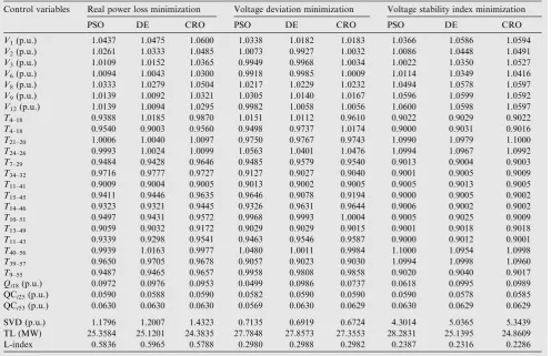
V1(p.u.) 1.0437 1.0475 1.0600 1.0338 1.0182 1.0183 1.0366 1.0586 1.0594
V2(p.u.) 1.0261 1.0333 1.0485 1.0073 0.9927 1.0032 1.0086 1.0448 1.0491
V3(p.u.) 1.0109 1.0152 1.0365 0.9949 0.9968 1.0034 1.0022 1.0350 1.0527
V6(p.u.) 1.0094 1.0043 1.0300 0.9918 0.9985 1.0009 1.0114 1.0349 1.0416
V8(p.u.) 1.0333 1.0279 1.0504 1.0217 1.0229 1.0232 1.0494 1.0578 1.0597
V9(p.u.) 1.0139 1.0092 1.0321 1.0305 1.0140 1.0167 1.0596 1.0599 1.0592
V12(p.u.) 1.0139 1.0094 1.0295 0.9982 1.0058 1.0056 1.0600 1.0598 1.0597
T4–18 0.9388 1.0185 0.9870 1.0151 1.0112 0.9610 0.9022 0.9029 0.9022
T4–18 0.9540 0.9003 0.9560 0.9498 0.9737 1.0174 0.9000 0.9031 0.9016
T21–20 1.0006 1.0040 1.0097 0.9750 0.9767 0.9743 1.0990 1.0979 1.1000 T24–26 0.9993 1.0024 1.0099 1.0563 1.0401 1.0476 1.0994 1.0967 1.0992
T7–29 0.9484 0.9428 0.9646 0.9485 0.9579 0.9540 0.9013 0.9004 0.9003
T34–32 0.9716 0.9777 0.9727 0.9127 0.9027 0.9040 0.9001 0.9005 0.9009 T11–41 0.9009 0.9004 0.9005 0.9013 0.9002 0.9005 0.9005 0.9013 0.9005 T15–45 0.9411 0.9446 0.9635 0.9646 0.9078 0.9194 0.9000 0.9005 0.9002 T14–46 0.9323 0.9321 0.9445 0.9326 0.9631 0.9644 0.9006 0.9002 0.9002 T10–51 0.9497 0.9431 0.9572 0.9968 0.9993 1.0004 0.9005 0.9025 0.9009 T13–49 0.9059 0.9032 0.9172 0.9029 0.9029 0.9015 0.9001 0.9018 0.9018 T11–43 0.9339 0.9298 0.9541 0.9463 0.9546 0.9587 0.9000 0.9012 0.9001 T40–56 0.9939 1.0163 0.9977 1.0480 1.0011 0.9984 1.1000 1.0954 1.0998 T39–57 0.9650 0.9705 0.9678 0.9057 0.9023 0.9030 1.0994 1.0998 1.0960
T9–55 0.9487 0.9465 0.9657 0.9958 0.9808 0.9858 0.9020 0.9040 0.9017
Qi18(p.u.) 0.0972 0.0976 0.0953 0.0499 0.0986 0.0737 0.0618 0.0995 0.0989
QCi25(p.u.) 0.0590 0.0588 0.0590 0.0582 0.0590 0.0590 0.0590 0.0578 0.0585
QCi53(p.u.) 0.0630 0.0630 0.0630 0.0569 0.0630 0.0629 0.0630 0.0629 0.0629
SVD (p.u.) 1.1796 1.2007 1.4323 0.7135 0.6919 0.6724 4.3014 5.0365 5.3439
TL (MW) 25.3584 25.1201 24.3835 27.7848 27.8573 27.3553 28.2831 25.1395 24.8609
TLBO [29], QOTLBO [29], SPEA[30], GA-1[31]and GA-2
[32]. The statistical results reported inTable 3 show that the best, worst and the average results obtained by CRO are near
about the same and the variation is negligible. These facts strongly demonstrate the robustness of the proposed CRO for the conventional ORPD problem. The worst and mean loss Table 8 Comparison of simulation results obtained by different algorithms with STATCOM.
Control variables Real power loss minimization Voltage deviation minimization Voltage stability index minimization
PSO DE CRO PSO DE CRO PSO DE CRO
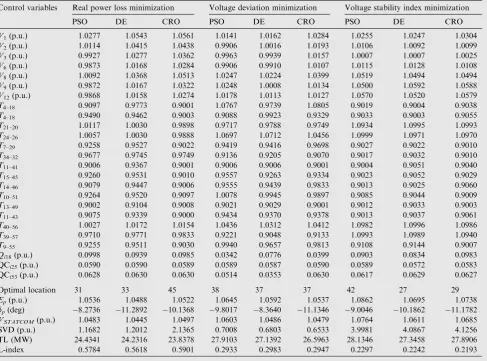
V1(p.u.) 1.0277 1.0543 1.0561 1.0141 1.0162 1.0284 1.0255 1.0247 1.0304
V2(p.u.) 1.0114 1.0415 1.0438 0.9906 1.0016 1.0193 1.0106 1.0092 1.0099
V3(p.u.) 0.9927 1.0277 1.0362 0.9963 0.9939 1.0157 1.0007 1.0007 1.0025
V6(p.u.) 0.9873 1.0168 1.0284 0.9906 0.9910 1.0107 1.0115 1.0128 1.0108
V8(p.u.) 1.0092 1.0368 1.0513 1.0247 1.0224 1.0399 1.0519 1.0494 1.0494
V9(p.u.) 0.9872 1.0167 1.0322 1.0248 1.0008 1.0134 1.0500 1.0592 1.0588
V12(p.u.) 0.9868 1.0158 1.0274 1.0178 1.0113 1.0127 1.0570 1.0520 1.0579
T4–18 0.9097 0.9773 0.9001 1.0767 0.9739 1.0805 0.9019 0.9004 0.9038
T4–18 0.9490 0.9462 0.9003 0.9088 0.9923 0.9329 0.9033 0.9003 0.9055
T21–20 1.0117 1.0030 0.9898 0.9717 0.9788 0.9749 1.0934 1.0995 1.0993 T24–26 1.0057 1.0030 0.9888 1.0697 1.0712 1.0456 1.0999 1.0971 1.0970
T7–29 0.9258 0.9527 0.9022 0.9419 0.9416 0.9698 0.9027 0.9022 0.9010
T34–32 0.9677 0.9745 0.9749 0.9136 0.9205 0.9070 0.9017 0.9032 0.9010 T11–41 0.9006 0.9367 0.9001 0.9006 0.9006 0.9001 0.9004 0.9051 0.9040 T15–45 0.9260 0.9531 0.9010 0.9557 0.9263 0.9334 0.9023 0.9052 0.9029 T14–46 0.9079 0.9447 0.9006 0.9555 0.9439 0.9833 0.9013 0.9025 0.9060 T10–51 0.9264 0.9520 0.9097 1.0078 0.9945 0.9897 0.9085 0.9044 0.9009 T13–49 0.9002 0.9104 0.9008 0.9021 0.9029 0.9001 0.9012 0.9033 0.9003 T11–43 0.9075 0.9339 0.9000 0.9434 0.9370 0.9378 0.9013 0.9037 0.9061 T40–56 1.0027 1.0172 1.0154 1.0436 1.0312 1.0412 1.0982 1.0996 1.0986 T39–57 0.9710 0.9771 0.9833 0.9221 0.9048 0.9133 1.0993 1.0989 1.0940
T9–55 0.9255 0.9511 0.9030 0.9940 0.9657 0.9813 0.9108 0.9144 0.9007
Qi18(p.u.) 0.0998 0.0939 0.0985 0.0342 0.0776 0.0399 0.0903 0.0834 0.0983
QCi25(p.u.) 0.0590 0.0590 0.0589 0.0589 0.0587 0.0590 0.0589 0.0572 0.0583
QCi53(p.u.) 0.0628 0.0630 0.0630 0.0514 0.0353 0.0630 0.0617 0.0629 0.0627
Optimal location 31 33 45 38 37 37 42 27 29
Ep(p.u.) 1.0536 1.0488 1.0522 1.0645 1.0592 1.0537 1.0862 1.0695 1.0738
dp(deg) 8.2736 11.2892 10.1368 9.8017 8.3640 11.1346 9.0046 10.1862 11.1782
VSTATCOM(p.u.) 1.0483 1.0445 1.0497 1.0603 1.0486 1.0479 1.0764 1.0611 1.0685
SVD (p.u.) 1.1682 1.2012 2.1365 0.7008 0.6803 0.6533 3.9981 4.0867 4.1256
TL (MW) 24.4341 24.2316 23.8378 27.9103 27.1392 26.5963 28.1346 27.3458 27.8906
L-index 0.5784 0.5618 0.5901 0.2933 0.2983 0.2947 0.2297 0.2242 0.2193
Table 7 Statistical comparison (50 trials) among various algorithms for IEEE 57-bus without STATCOM.
Real power loss minimization
Techniquesfi PSO PSO-w PSO-cf CLPSO SPSO CGA AGA DE L-SACP-DE SOA GSA CRO
Best loss p.u.) 0.2536 0.2597 0.2479 0.2580 0.2742 0.2671 0.2581 0.2512 0.2732 0.2462 0.2444 0.2438 Mean loss (p.u.) 0.2635 0.2839 0.2971 0.2733 0.3070 0.3232 0.2967 0.2618 0.3434 0.2574 0.2483 0.2443 Worst loss (p.u.) 0.2774 0.3249 0.3932 0.3400 0.3862 0.4197 0.3698 0.2730 0.4439 0.2875 0.2816 0.2451
Voltage deviation minimization
Techniques OGSA[35] PSO DE CRO
Best VD 0.6982 0.7135 0.6919 0.6724
Mean VD NA 0.7206 0.7047 0.6793
Worst VD NA 0.7375 0.7133 0.6738
Voltage stability index minimization
Techniques MOPSO-2[36] MOIPSO[36] MOCIPSO[36] PSO DE CRO
Best L index 0.28834 0.24087 0.23291 0.2387 0.2316 0.2286
Mean L index NA NA NA 0.2422 0.2388 0.2293
of SPEA, GA-I and GA-2 are not available (NA) in the literature.
(ii) ORPD with STATCOM
In order to check the feasibility of the proposed method for complicated network, it is applied to solve ORPD with STATCOM of the same test system. The simulation results of transmission loss, the controlled variables, optimal position of STATCOM and its voltage rating obtained by PSO, DE and CRO are shown inTable 4. The simulation results show that using STATCOM the transmission loss has substantially reduced for all the algorithms. Moreover, the results indicate that the proposed CRO algorithm gives more reduction in loss (4.5297 MW) compared to PSO (4.5802 MW) and DE (4.5493 MW). The convergence of minimal transmission loss with evolution generations shown inFig. 3certifies the results
ofTable 4 vividly. Especially, CRO algorithm can not only
maintain the diversity of the objective function solutions at the beginning of searching but also converge in the best solu-tion at the later searching. The statistical results of CRO, DE and PSO are reported inTable 5. FromTable 5it is very evident that CRO not only has found the highest quality results among the all algorithms compared, but also possesses the highest probability of finding the better solution for the problem under consideration.
Case B: Voltage deviation minimization
The results obtained for this objective function by PSO, DE and CRO without and with STATCOM devices are reported in 5th, 6th and 7th columns ofTables 2 and 4, respectively. It is observed from the simulation results that voltage devia-tion is improved by incorporating STATCOM from 0.1086 p.u. to 0.1013 p.u. by PSO, from 0.1029 p.u. to 0.0928 p.u. by DE and from 0.0849 p.u. to 0.0803 p.u. by CRO method. Moreover, it is observed that voltage deviation using proposed CRO is better as compared to that obtained by PSO and DE algorithms. The statistical results for voltage deviation minimization objective illustrated in Tables 3 and 5, show the superiority of the proposed CRO method over other approaches.
Case C: Minimization of L-index voltage stability
To further investigate the efficiency of the proposed CRO method, it is applied on the same IEEE 30-bus system to min-imize voltage stability index. The 8th–10th columns ofTables 2 and 4show the optimal settings of control variables, optimal locations and optimal parameter setting of STATCOM obtained by applying PSO, DE and CRO techniques for nor-mal and FACTs based ORPD problem. For voltage stability
index minimization objective, before using FACTS devices in the transmission network, the L-index obtained using PSO, DE and CRO was 0.1210 p.u., 0.1198 p.u. and 0.1156 p.u., respectively. However, after installing STATCOM with opti-mal settings in the optimized location using PSO, DE and CRO, the voltage stability index in the different buses is signif-icantly reduced. However, the best L-index is obtained using CRO method for both the cases (i.e. without and with STATCOM).
4.2. IEEE 57-bus system
In order to assess the effectiveness and robustness of the pro-posed CRO method, a larger test system consisting of 57 buses Table 9 Statistical comparison (50 trials) among various methods for IEEE 57-bus with STATCOM.
Techniquesfi Real power loss minimization Voltage deviation minimization Voltage stability index minimization
PSO DE CRO PSO DE CRO PSO DE CRO
Best 24.4341 24.2316 23.8378 0.7008 0.6803 0.6533 0.2297 0.2242 0.2193
Mean 25.9073 25.6371 23.8904 0.7075 0.6891 0.6541 0.2378 0.2316 0.2204
Worst 27.0068 26.9117 23.9655 0.7183 0.7011 0.6586 0.2405 0.2480 0.2237
0 20 40 60 80 100
24 26 28 30 32 34
Generation Cycles
Transmission Loss (MW)
DE
PSO
CRO
Figure 4 Convergence characteristics of different algorithms for transmission loss with STATCOM (IEEE 57-bus system).
0 20 40 60 80 100
0.22 0.24 0.26 0.28 0.3 0.32 0.34 0.36
Generation Cycles
Voltage Stability Index
DE
PSO
CRO
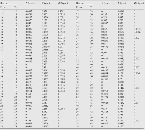
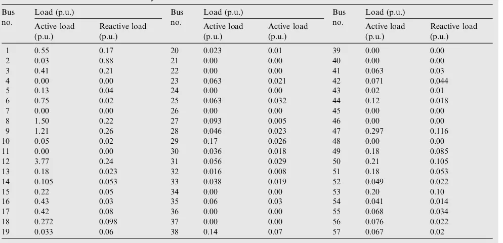
with and without STATCOM is considered to solve ORPD problem. This system (IEEE 57-bus) consists of seven genera-tor buses (the bus 1 is the slack bus and buses 2, 3, 6, 8, 9 and 12 are PV buses), fifty load buses and 80 branches, in which branches (4–12, 20–21, 24–26, 7–29, 32–34, 11–41, 15–45, 14–46, 10–51, 13–49, 11–43, 40–56, 39–57, and 9–55) are tap changing transformers. In addition, buses 8, 25 and 53 are selected as shunt compensation buses. The base load of the sys-tem is 1272 MW and 298 MVAR. The full syssys-tem data adopted from [38] are listed in Tables A4–A6. The voltage magnitude limits of all buses are set to 0.94 p.u. for lower bound and to 1.06 p.u. for upper bound. In this study, the allowed steps for tap changers are between 0.9 and 1.1 p.u., the allowed voltage changes are between 0.95 and 1.05. In order to test and validate the robustness of the proposed
algorithm, simulations are carried out for conventional ORPF problem and STATCOM based ORPD problems.
Case A: Transmission loss minimization
(i) ORPD without STATCOM device
The optimal settings of control variables obtained by CRO, PSO and DE for this case are illustrated inTable 6. It is noted that all the state variables and control variables are in their specified limits. To assess the potential of the proposed approach, a comparison among the results obtained by the CRO, DE, PSO approaches and those reported in the litera-ture are carried out. The results of this comparison are given inTable 7. It is worth mentioning that the comparison is car-ried out with the same control variable limits, and other system
Table A1 Transmission line data of IEEE 30 bus system.
Bus no. R(p.u.) X(p.u.) B/2 (p.u.) Bus no. R(p.u.) X(p.u.) B/2 (p.u.)
From To From To
1 2 0.0192 0.0575 0.0264 15 18 0.1073 0.2185 0.0000
1 3 0.0452 0.1852 0.0204 18 19 0.0639 0.1292 0.0000
2 4 0.057 0.1737 0.0184 19 20 0.0340 0.0680 0.0000
3 4 0.0132 0.0379 0.0042 10 20 0.0936 0.2090 0.0000
2 5 0.0472 0.1983 0.0209 10 17 0.0324 0.0845 0.0000
2 6 0.0581 0.1763 0.0187 10 21 0.0348 0.0749 0.0000
4 6 0.0119 0.0414 0.0045 10 22 0.0727 0.1499 0.0000
5 7 0.0460 0.1160 0.0102 21 22 0.0116 0.0236 0.0000
6 7 0.0267 0.0820 0.0085 15 23 0.1000 0.2020 0.0000
6 8 0.0120 0.0420 0.0045 22 24 0.1150 0.1790 0.0000
6 9 0.0000 0.2080 0.000 23 24 0.1320 0.2700 0.0000
6 10 0.0000 0.5560 0.000 24 25 0.1885 0.3292 0.0000
9 11 0.0000 0.2080 0.000 25 26 0.2544 0.3800 0.0000
9 10 0.0000 0.1100 0.000 25 27 0.1093 0.2087 0.0000
4 12 0.0000 0.2560 0.000 28 27 0.0000 0.3960 0.0000
12 13 0.0000 0.1400 0.000 27 29 0.2198 0.4153 0.0000
12 14 0.1231 0.2559 0.000 27 30 0.3202 0.6027 0.0000
12 15 0.0662 0.1304 0.000 29 30 0.2399 0.4533 0.0000
12 16 0.0945 0.1987 0.000 8 28 0.0636 0.2000 0.0214
14 15 0.2210 0.1997 0.000 6 28 0.0169 0.0599 0.0065
16 17 0.0524 0.1923 0.000
Table A2 Load data of IEEE 30 bus system.
Bus no.
Load (p.u.) Bus
no.
Load (p.u.) Bus
no.
Load (p.u.)
Active load (p.u.)
Reactive load (p.u.)
Active load (p.u.)
Reactive load (p.u.)
Active load (p.u.)
Reactive load (p.u.)
1 0 0 11 0.0000 0.0000 21 0.1750 0.1120
2 0.2170 0.1270 12 0.1120 0.0750 22 0.0000 0.0000
3 0.0240 0.0120 13 0.0000 0.0000 23 0.0320 0.0160
4 0.0760 0.0160 14 0.0620 0.0160 24 0.0870 0.0670
5 0.9420 0.1900 15 0.0820 0.0250 25 0.0000 0.0000
6 0.0000 0.0000 16 0.0350 0.0180 26 0.0350 0.0230
7 0.2280 0.1090 17 0.0900 0.0580 27 0.0000 0.0000
8 0.3000 0.3000 18 0.0320 0.0090 28 0.0000 0.0000
9 0.0000 0.0000 19 0.0950 0.0340 29 0.0240 0.0090
data.Table 7clearly shows that the CRO technique outper-forms PSO, PSO-w, PSO-cf, CLPSO, SPSO, CGA, AGA, DE, L-SACP-DE, SOA and GSA.
(ii) ORPD with STATCOM device
The effectiveness of the CRO method is further evaluated by implementing the proposed method on IEEE 57-bus system
to minimize transmission loss STATCOM based power system network. The detailed simulation results of CRO, PSO and DE are illustrated in Table 8. It is found that the active power losses achieved by the proposed CRO algorithm is equal 23.8378 MW while it is equal to 24.2316 MW and 24.4341 MW for DE and PSO methods, respectively. As can be derived from the results, the proposed algorithm gives the best performance in comparison with the PSO and DE meth-ods. Moreover, to verify the robustness, the CRO, DE and PSO algorithms are executed for 50 trials with different start-ing points.Table 9presents the minimum, maximum and aver-age transmission loss produced by the proposed algorithm comparing with the other reported results. It is worth mention-ing that the best, mean and the worst loss obtained by the pro-posed CRO method are better than those obtained by the DE and PSO methods, which clearly suggest the robustness of the proposed CRO method. The convergence of optimal solution using DE, PSO and CRO is shown inFig. 4. It is found from Table A3 Generators’ input data of IEEE 30 bus system.
Bus no. Pint(MW) Qmin(Mvar) Qmax(Mvar)
1 Slack power 0.00 10.0
2 80.0 40.0 50.0
5 50.0 40.0 40.0
8 20.0 10.0 40.0
11 20.0 6.0 24.0
13 20.0 6.0 24.0
Table A4 Transmission line data of IEEE 57 bus system.
Bus no. R(p.u.) X(p.u.) B/2 (p.u.) Bus no. R(p.u.) X(p.u.) B/2 (p.u.)
From To From To
1 2 0.0083 0.028 0.129 7 29 0 0.0648 0
2 3 0.0298 0.085 0.0818 25 30 0.135 0.202 0
3 4 0.0112 0.0366 0.038 30 31 0.326 0.497 0
4 5 0.0625 0.132 0.0258 31 32 0.507 0.755 0
4 6 0.043 0.148 0.0348 32 33 0.0392 0.036 0
6 7 0.02 0.102 0.0276 34 32 0 0.953 0
6 8 0.0339 0.173 0.047 34 35 0.052 0.078 0.0032
8 9 0.0099 0.0505 0.0548 35 36 0.043 0.0537 0.0016
9 10 0.0369 0.1679 0.044 36 37 0.029 0.0366 0
9 11 0.0258 0.0848 0.0218 37 38 0.0651 0.1009 0.002
9 12 0.0648 0.295 0.0772 37 39 0.0239 0.0379 0
9 13 0.0481 0.158 0.0406 36 40 0.03 0.0466 0
13 14 0.0132 0.04340 0.011 22 38 0.0192 0.0295 0
13 15 0.0269 0.0869 0.023 11 41 0 0.749 0
1 15 0.0178 0.091 0.0988 41 42 0.207 0.352 0
1 16 0.0454 0.206 0.0546 41 43 0 0.412 0
1 17 0.0238 0.108 0.0286 38 44 0.0289 0.0585 0.002
3 15 0.0162 0.053 0.0544 15 45 0 0.1042 0
4 18 0 0.555 0 14 46 0 0.0735 0
4 18 0 0.43 0 46 47 0.023 0.068 0.0032
5 6 0.0302 0.0641 0.0124 47 48 0.0182 0.0233 0
7 8 0.0139 0.0712 0.0194 48 49 0.0834 0.129 0.0048
10 12 0.0277 0.1262 0.0328 49 50 0.0801 0.128 0
11 13 0.0223 0.0732 0.0188 50 51 0.1386 0.22 0
12 13 0.0178 0.058 0.0604 10 51 0 0.0712 0
12 16 0.018 0.0813 0.0216 13 49 0 0.191 0
12 17 0.0397 0.179 0.0476 29 52 0 0.1442 0.187
14 15 0.0171 0.0547 0.0148 52 53 0.0762 0.0984 0
18 19 0.461 0.685 0 53 54 0.1878 0.232 0
19 20 0.283 0.434 0 54 55 0.1732 0.2265 0
21 20 0 0.7767 0 11 43 0 0.153 0
21 22 0.0736 0.117 0 44 45 0.0624 0.1242 0.004
22 23 0.0099 0.0152 0 40 56 0 1.195 0
23 24 0.166 0.256 0.0084 56 41 0.553 0.549 0
24 25 0 1.182 0 56 42 0.2125 0.354 0
24 25 0 1.23 0 39 57 0 1.355 0
24 26 0 0.0473 0 57 56 0.174 0.26 0
26 27 0.165 0.254 0 38 49 0.115 0.177 0.003
27 28 0.0618 0.0954 0 38 48 0.0312 0.0482 0
the convergence graphs that for CRO only about 45 iterations are needed to find the optimal solution. However, for both DE and PSO, almost 85 iterations are required to achieve optimal results.
Case B: Voltage deviation minimization
Here, PSO, DE and CRO approaches are applied on the same test system with the objective of voltage deviation mini-mization without and with STATCOM devices. The corre-sponding results obtained by the different methods are listed in the 5th–7th columns ofTables 6 and 8. The voltage devia-tion value obtained by PSO, DE and CRO methods is 0.7135 p.u., 0.6919 p.u. and 0.6724 p.u., respectively, for ORPD without FACTS. After incorporating the STATCOM, voltage deviation value obtained by PSO, DE and CRO methods is 0.7008 p.u., 0.6803 p.u. and 0.6533 p.u., respectively. This clearly suggests that voltage deviation has been significantly reduced by incorporating STATCOM in optimal location. However, the simulation results indicate that reduction of voltage deviation obtained by CRO is best among all the discussed algorithms for both normal ORPD and FACTS based ORPD problems. This fact clearly suggests that CRO outperforms PSO and DE in terms of solution quality.
Case C: Minimization of L-index voltage stability
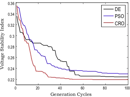
Finally, PSO, DE and CRO techniques are applied for L-index minimization on IEEE 57-bus system to test the superi-ority of the proposed CRO approach. The optimal control variables, TL, VD, and L-index values obtained using PSO, DE and CRO approaches in the IEEE 57-bus power system for L-index minimization objective of normal ORPD and STATCOM based ORPD are elaborated in the columns 8th– 10th of Tables 6 and 8, respectively. The results clearly
demonstrate that the L-index reduction accomplished using the CRO approach is better than that obtained by the other approaches. Hence, the conclusion can be drawn that CRO is better than all the other listed algorithms in terms of global search capacity and local search precision. Furthermore, it can be seen that all the control variables optimized by the various discussed methods are acceptably kept within the limits.Fig. 5
shows the convergence performance of algorithms with the evolution process. It shows that, compared with PSO, and DE, CRO has faster convergence speed and needs lesser itera-tion cycles to achieve the optimal L-index level. The statistical results of L-index minimization objective for normal and STATCOM based ORPD problem are illustrated in the last three columns ofTables 7 and 9, respectively. The statistical results clearly suggest the robustness of the proposed methods over other discussed methods.
5. Conclusion
Chemical reaction optimization (CRO) has proven to be an efficient nonlinear optimization technique for solving different types of real world problems of various field of engineering. In this article CRO is used to find the optimal location of STATCOM for solving optimal reactive power dispatch (ORPD) problem. Minimization of the transmission loss, improvement of the voltage profile and voltage stability are considered as the objective function to evaluate the system per-formance. It is observed that the STATCOM can reduce the transmission loss, voltage deviation and voltage stability index of a power system network effectively. Moreover, for all the three different objectives, CRO produces better solutions than so far best known results by any other method. Furthermore, from the statistical comparative results, it is found that the proposed CRO algorithm is robust and suitable for sizing and locating STATCOM devices in power system transmission system. Considering all these results of the study for ORPD
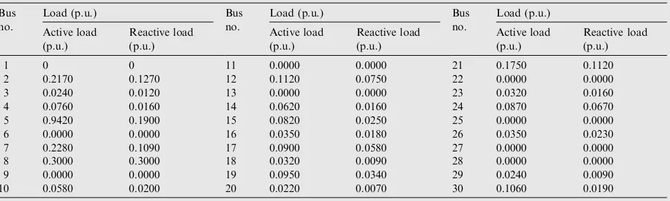
Table A5 Load data of IEEE 57 bus system.
Bus no.
Load (p.u.) Bus
no.
Load (p.u.) Bus
no.
Load (p.u.)
Active load (p.u.)
Reactive load (p.u.)
Active load (p.u.)
Active load (p.u.)
Active load (p.u.)
Reactive load (p.u.)
1 0.55 0.17 20 0.023 0.01 39 0.00 0.00
2 0.03 0.88 21 0.00 0.00 40 0.00 0.00
3 0.41 0.21 22 0.00 0.00 41 0.063 0.03
4 0.00 0.00 23 0.063 0.021 42 0.071 0.044
5 0.13 0.04 24 0.00 0.00 43 0.02 0.01
6 0.75 0.02 25 0.063 0.032 44 0.12 0.018
7 0.00 0.00 26 0.00 0.00 45 0.00 0.00
8 1.50 0.22 27 0.093 0.005 46 0.00 0.00
9 1.21 0.26 28 0.046 0.023 47 0.297 0.116
10 0.05 0.02 29 0.17 0.026 48 0.00 0.00
11 0.00 0.00 30 0.036 0.018 49 0.18 0.085
12 3.77 0.24 31 0.056 0.029 50 0.21 0.105
13 0.18 0.023 32 0.016 0.008 51 0.18 0.053
14 0.105 0.053 33 0.038 0.019 52 0.049 0.022
15 0.22 0.05 34 0.00 0.00 53 0.20 0.10
16 0.43 0.03 35 0.06 0.03 54 0.041 0.014
17 0.42 0.08 36 0.00 0.00 55 0.068 0.034
18 0.272 0.098 37 0.00 0.00 56 0.076 0.022
problems with different characteristics, dimensions, and con-straints it can be concluded that CRO performs better, at least matching many of the previously reported methods.
Appendix A
SeeTables A1–A6.
References
[1] Hingorani NG, Gyugyi L. Understanding FACTS: concepts and technology of flexible AC transmission systems. New York: IEEE Press; 2001.
[2]Galiana FD, Almeida K, Toussaint M, Griffin J, Atanackovic D, Ooi BT, McGillis DT. Assessment and control of the impact of FACTS devices on power system performance. IEEE Trans Power Syst 1996;11(4):1931–6.
[3]Urdaneta AJ, Gomez JF, Sorrentino E, Flores L, Diaz R. A hybrid genetic algorithm for optimal reactive power planning based upon successive linear programming. IEEE Trans Power Syst 1999;14(4):1292–8.
[4]Grudinin N. Reactive power optimization using successive quadratic programming method. IEEE Trans Power Syst 1998;13(4):1219–25.
[5]Lai LL, Ma JT. Application of evolutionary programming to reactive power planning-comparison with nonlinear programming approach. IEEE Trans Power Syst 1997;12(1):198–206.
[6] Kim DH, Lee JH, Hong SH, Kim SR. A mixed-integer programming approach for the linearized reactive power and voltage control-comparison with gradient projection approach. In: International conference on energy management and power delivery, proceed of EMPD, vol. 1; 1998. p. 67–72.
[7]Amjady N, Ansari MR. Non-convex security constrained optimal power flow by a new solution method composed of Benders decomposition and special ordered sets. Int Trans Electr Energy Syst 2014;24(6):842–57.
[8]Venkatesh P, Gnanadas R, Padhy NP. Comparison and applica-tion of evoluapplica-tionary programming techniques to combined economic emission dispatch with line flow constrained. IEEE Trans Power Syst 2003;18:688–97.
[9]Wei Y, Fang L, Chung CY, Wong KP. A hybrid genetic algorithm-interior point method for optimal reactive power flow. IEEE Trans Power Syst 2006;21(3):1163–9.
[10]Zhihuan L, Yinhong L, Xianzhong D. Non-dominated sorting genetic algorithm-II for robust multi-objective opti-mal reactive power dispatch. IET Gener Transm Distrib 2010;4(9):1000–8.
[11] Keyan L, Wanxing S, Yunhua L. Research on reactive power optimization based on adaptive genetic simulated annealing algorithm. In: International conference on power system tech, Power Con; 2006. p. 1–6.
[12] Guo L, Ding X, Chen G, Song J, Cui Q, Liu W. A combination strategy for reactive power optimization based on model of soft constrain considered interior point method and genetic
simulated annealing algorithm. In: International conference on information science and management engineering (ISME), vol. 2; 2010. p. 151–4.
[13] Wennan L, Yihua L, Xingtao X, Maojun I. Reactive power optimization in area power grid based on improved Tabu search algorithm. In: Third international conference on electric utility deregulation and restructuring and power technologies, DRPT; 2008. p. 1472–77.
[14] Zou Y. Optimal reactive power planning based on improved Tabu search algorithm. In: International Conference on Electrical and Control Engineering (ICECE); 2010. p. 3945–8.
[15] Shaheen HI, Rashed GI, Cheng SJ. Application of differential evolution algorithm for optimal location and parameters setting of UPFC considering power system security. Eur Trans Electr Power 2009;19(7):911–32.
[16] Chao-Ming H, Shin-Ju C, Yann-Chang H, Sung-Pei Y. Optimal active-reactive power dispatch using an enhanced differential evolution algorithm. In: 6th IEEE Conference on Industrial Electronics and Applications (ICIEA); 2011. p. 1869–74. [17] Zhao B, Guo CX, Cao YJ. A multiagent-based particle swarm
optimization approach for optimal reactive power dispatch. IEEE Trans Power Syst 2005;20(2):1070–8.
[18] Niknam T, Narimani MR, Jabbari M. Dynamic optimal power flow using hybrid particle swarm optimization and simulated annealing. Int Trans Electr Energy Syst 2013;23(7):975–1001. [19] Karaboga D, Basturk B. A powerful and efficient algorithm for
numerical function optimization: artificial bee colony (ABC) algorithm. J Global Optim 2007;39(3):459–71.
[20] Sirjani R, Mohamed A, Shareef H. Optimal allocation of shunt Var compensators in power systems using a novel global harmony search algorithm. Int J Electr Power Energy Syst 2012; 43(1):562–72.
[21] Saravanan M, Raja M, Slochanal SMR, Venkatesh P, Abraham JPS. Application of particle swarm optimization technique for optimal location of FACTS devices considering cost of installa-tion and system loadability. Electr Pow Syst Res 2007; 77(3):276–83.
[22] Xiao Y, Song YH. Power flow studies of a large practical power network with embedded facts devices using improved optimal multiplier Newton–Raphson method. Eur Trans Electr Power 2001;11(4):247–56.
[23] Ghadir R, Reshma SR. Power flow model/calculation for power systems with multiple FACTS controllers. Electr Power Syst Res 2007;77:1521–31.
[24] Lam AYS, Li VOK. Chemical-reaction-inspired metaheuristic for optimization. IEEE Trans Evol Comput 2010;14(3):381–99. [25] Li JQ, Pan QK. Chemical-reaction optimization for flexible
job-shop scheduling problems with maintenance activity. Appl Soft Comput 2012;12(9):2896–912.
[26] Szeto WY, Wang Y, Wong SC. The chemical reaction optimiza-tion approach to solving the environmentally sustainable network design problem. Comput-Aided Civil Inf Eng; 2013.
[27] Dai C, Chen W, Zhu Y, Zhang X. Reactive power dispatch considering voltage stability with seeker optimization algorithm. Electric Power Syst Res 2009;79:1462–71.
[28] Roy PK, Mandal B, Bhattacharya K. Gravitational search algorithm based optimal reactive power dispatch for voltage stability enhancement. Electr Power Compon Syst 2012;40: 956–76.
[29] Mandal B, Roy PK. Optimal reactive power dispatch using quasi-oppositional teaching learning based optimization. Int J Electr Power Energy Syst 2013;53:123–34.
[30] Abido MA. Multiobjective optimal VAR dispatch using strength pareto evolutionary algorithm. Vancouver, BC, Canada: IEEE Congress on Evolutionary Computation; 2006.
[31] Subburaj P, Sudha N, Rajeswari K, Ramar K, Ganesan L. Optimum reactive power dispatch using genetic algorithm. Acad Open Internet J 2007:21.
Table A6 Generators’ input data of IEEE 57 bus system.
[32]Devaraj D, Roselyn JP. Genetic algorithm based reactive power dispatch for voltage stability improvement. Int J Electr Power Energy Syst 2010;32(10):1151–6.
[33]Duraira S, Kannan PS, Devaraj D. Multi-objective VAR dispatch using particle swarm optimization. Emerg Electr Power Syst 2005;4(1).
[34]Abou El Ela AA, Abido MA, Spea SR. Differential evolution algorithm for optimal reactive power dispatch. Electr Power Syst Res 2011;81(2):458–64.
[35]Shaw B, Mukherjee V, Ghoshal SP. Solution of reactive power dispatch of power systems by an opposition-based gravitational search algorithm. Int J Electr Power Energy Syst 2014;55:29–40. [36]Chen G, Liu L, Song P, Du Y. Chaotic improved PSO-based multi-objective optimization for minimization of power losses and L index in power systems. Energy Convers Manage 2014;86: 548–60.
[37]Basu M. Optimal power flow with FACTS devices using differ-ential evolution. Int J Electr Power Energy Syst 2008;30(2):150–6. [38] Zimmerman RD, Murillo-Sanchez CE, Gan D. Matlab power system simulation package (version 3.1b2) 2006 <http://www. pserc.cornell.edu/matpower/>.
Susanta Duttawas born in 1976 at Bankura, West Bengal, India. He received the BE degree in Electrical Engineering from Dr. B.C. Roy Engineering College, Durgapur, Burdwan, India in 2004; ME degree from NIT Durgapur, India in 2007. Presently he is working as Assistant Professor in the depart-ment of Electrical Engineering, Dr. B.C. Roy Engineering College, Durgapur, India. His field of research interest includes Economic Load Dispatch, Optimal Power flow, FACTS, Automatic Generation Control, Evolutionary computing techniques.
Dr. Provas Kumar Roywas born in 1973 at Mejia, Bankura, West Bengal, India. He received the BE degree in Electrical Engineering from R.E. College, Durgapur, Burdwan, India in 1997; ME degree in Electrical Machine from Jadavpur University, Kolkata, India in 2001 and PhD from NIT Durgapur in 2011. Presently he is working as Professor in the department of Electrical Engineering, Dr. B.C. Roy Engineering College, Durgapur, India. He has published more than 15 research papers in international journals. His field of research interest includes Economic Load Dispatch, Optimal Power flow, FACTS, Unit Commitment, Automatic Generation Control, Power System Stabilizer and Evolutionary computing techniques.