MODELLING THE RELATIONSHIP BETWEEN LAND SURFACE TEMPERATURE
AND LANDSCAPE PATTERNS OF LAND USE LAND COVER CLASSIFICATION
USING MULTI LINEAR REGRESSION MODELS
A. M. Bernales a, J. A. Antolihao a, C. Samonte a, F. Campomanes a, *, R. J. Rojas a, A. M. dela Serna a, J. Silapan b a
University of the Phlippines Cebu Phil-LiDAR 2, Gorordo Avenue, Lahug, Cebu City – (maebernales, an2antolihao, samonte.cristina, enzo.campomanesv, raynardrojas, alexismariedelaserna)@gmail.com
b
University of the Phlippines Cebu, Gorordo Avenue, Lahug, Cebu City – [email protected] Commission VIII, WG VIII/8
KEY WORDS: Land Surface Temperature, Land Use Land Cover, Multiple Linear Regression, LiDAR, Spatial Metrics
ABSTRACT:
The threat of the ailments related to urbanization like heat stress is very prevalent. There are a lot of things that can be done to lessen the effect of urbanization to the surface temperature of the area like using green roofs or planting trees in the area. So land use really matters in both increasing and decreasing surface temperature. It is known that there is a relationship between land use land cover (LULC) and land surface temperature (LST). Quantifying this relationship in terms of a mathematical model is very important so as to provide a way to predict LST based on the LULC alone. This study aims to examine the relationship between LST and LULC as well as to create a model that can predict LST using class-level spatial metrics from LULC. LST was derived from a Landsat 8 image and LULC classification was derived from LiDAR and Orthophoto datasets. Class-level spatial metrics were created in FRAGSTATS with the LULC and LST as inputs and these metrics were analysed using a statistical framework. Multi linear regression was done to create models that would predict LST for each class and it was found that the spatial metric “Effective mesh size” was a top predictor for LST in 6 out of 7 classes. The model created can still be refined by adding a temporal aspect by analysing the LST of another farming period (for rural areas) and looking for common predictors between LSTs of these two different farming periods.
1. INTRODUCTION
Land Surface Temperature (LST) is a very important measure in urban areas because as it increases, the possibilities of drought and heat stress also increase. It has been found that the temperatures are indeed greater in urban areas compared to rural areas (Sundara Kumar et al., 2012).
It is clear that the main cause of the increasing temperatures is urbanization or the transformation of natural surfaces to buildings and other structures. These natural surfaces are often composed of plants and soil so they release water vapour that keeps the air cool in the area. On the other hand, materials that are being used as roofs of buildings have different thermal properties which absorbs more of the sun‟s energy thus results to high temperature in the urban area.
Heat stress is a very big issue especially in urban areas and also in places where drought could occur. Areas in and around cities are generally warmer than most rural areas which should alarm people in those areas of the possibility of heat stress and its advanced effects like heat stroke which sometimes could be fatal. Furthermore, continuous urban development reduces vegetative cover and adds more surfaces that absorb heat like rooftops and paved roads. This also adds to the already growing harmful effect of climate change. It is known that there is indeed a relationship between land use and LST. Therefore, it is also very important to have a way to model LST based on Land Use Land Cover (LULC) so this relationship can be quantified. This model can be included in urban planning especially in plans of major urbanization to see the effect it would have on the LST in the area.
2. OBJECTIVES
This study aims to derive land surface temperature from a single Landsat 8 image and examine the effects of landscape patterns from LULC classification on surface temperature and create a regression model to predict surface temperature from class-level spatial metrics. The study also aims to develop a statistical framework to be used in analysing these relationships.
3. DATA AND METHODS
3.1 Study Area
The study site that was selected for this study was an area in Talisay City, Negros Occidental, Philippines that showed the contrast between urban and rural land classes.
Figure 1. Orthophoto of the study site taken in June 2014
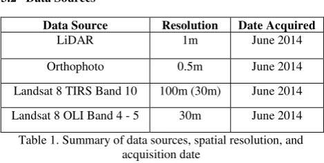
3.2 Data Sources
Data Source Resolution Date Acquired
LiDAR 1m June 2014
Orthophoto 0.5m June 2014
Landsat 8 TIRS Band 10 100m (30m) June 2014 Landsat 8 OLI Band 4 - 5 30m June 2014 Table 1. Summary of data sources, spatial resolution, and
acquisition date
The Landsat 8 image was taken during the period just before harvest season where crops are almost fully grown and ready to be harvested. The Landsat 8 image was taken around 02:05 AM local time and it was also made sure to have little to no cloud cover or haze in the study area so as not to distort any calculations for land surface temperature.
3.3 Land Surface Temperature (LST) Derivation
LST was derived from the Landsat 8 image. Only band 10 was used because for single channel methods, LST derived from band 10 gives higher accuracy than that of band 11 (Yu et al, 2014). The following equation was used to convert the digital number (DN) of Landsat 8 TIR band 10 into spectral radiance (USGS, 2015):
Lλ = ML * Qcal + AL (1)
where Lλ = spectral radiance Qcal = digital number (DN).
ML = radiance multiplicative scaling factor for the band (RADIANCE_MULT_BAND_n from the metadata)
AL = radiance additive scaling factor for the band (RADIANCE_ADD_BAND_n from the metadata)
The spectral radiance is then converted to brightness temperature, which is the at-satellite temperature (TB) under an assumption of unity emissivity using the following equation (USGS, 2015):
TB =
⁄ (2)
where TB = at-satellite brightness temperature in Kelvin (K) K1 and K2 = band-specific thermal conversion constants from the metadata
Next, NDVI is computed using the NIR and Red band of the Landsat 8 image since it will be used in determining land surface emissivity (LSE). NDVI is calculated using the following equation (Tucker, 1979):
(3)
In order to get the LSE, the vegetation proportion is obtained using the following equation (Carlson & Ripley, 1997):
PV = [ ⁄ ] (4) (3) where PV = vegetation proportion
NDVI = normalised difference vegetation index NDVImin = minimum NDVI value
NDVImax = maximum NDVI value
LSE is then computed using the following equation (Sobrino et al., 2004):
LSE = (5)
LST can now be computed (in degrees Celsius) using the at-satellite brightness temperature and the land surface emissivity in this equation (Artis & Carnahan, 1982):
LST = ⁄ (6)
where LST = land surface temperature
TB is the at-satellite brightness temperature
is the wavelength of emitted radiance ( = 11.5µm) (Markham & Barker, 1985)
ρ = h * c/σ (1.438 * 10-2 m K) σ = Boltzmann constant (1.38 * 10-23
J/K) h = Planck‟s constant (6.626 * 10-34
Js) c = velocity of light (2.998 * 108 m/s) 3.4 Land Use Land Cover Classification
Detailed land use land cover classes were obtained by using LiDAR data and orthophotos with an object-based image analysis (OBIA) approach. Different features from the LiDAR data and orthophotos were created and used to both segment and classify the study area. Using the pit-free canopy height model (CHM) (Khosravipour et al, 2014), the unclassified image was separated into ground and non-ground objects by using contrast split segmentation (Trimble, 2014). The ground and non-ground objects were further segmented using multiresolution segmentation (Trimble, 2014) and refinement was done by removing small and irrelevant objects. Training and validation points were collected by visual interpretation using the orthophoto and LiDAR derivatives like CHM and intensity. After collection, the classes found in the study area were Sugarcane (SC), Rice (Ri), Mango, Fallow (Fa), Bare Land (BL), Builtup (Bu), Grassland (Gr), Road (Rd), Trees (Tree), and Water. A support vector machine (SVM) was used to classify the segmented image and the initial result was refined using neighbourhood features and geometric features like area to get a more homogenous output. Smaller insignificant objects were merged with their larger neighbours. Accuracy assessment was done using the collected validation points.
3.5 Spatial Metric Computation
The relationship of LST derived from Landsat 8 and land cover class-level spatial metrics were investigated using simple linear regression. Preprocessing of the land cover polygons was done in ArcMap 10.3. The study site with an area of 3480 x 3570 meters was divided into 30 x 30 meter grids. Each grid had a 2 meter buffer which was considered as its edge. The land cover polygons were clipped according to each grid and were rasterized afterwards.
The rasters including their edges were then used as input in FRAGSTATS, a spatial analysis tool (McGarigal et al, 2012). It was utilized to derive the class-level spatial metrics of the land cover polygons in the study area. A total of 73 spatial metrics were tested in FRAGSTATS. Table 2 shows the class-level spatial metrics that were derived.
Metric Acronym
Area and edge metrics Total (class) area CA Percentage of landscape PLAND Largest patch index LPI
Total edge TE
Edge density ED
Patch area distribution AREA_MN, _AM, _MD, _RA, _SD, _CV
Shape index distribution SHAPE_MN, _AM, _MD_RA,_SD,_CV Fractal dimension index FRAC_MN, _AM,
_MD_RA,_SD,_CV
Landscape division index DIVISION
Splitting index SPLIT
Landscape shape index LSI
Normalized LSI NLSI
Patch Density PD
Number of patches NP
Patch Cohesion Index COHESION Effective mesh size MESH Euclidean nearest
‘median’, ’range’, ‘standard deviation’, and ‘coefficient of variation’, respectively.
Table 2. Class-level spatial metrics derived from FRAGSTATS 3.6 Statistics
Before proceeding to any type of statistical analysis, checking for the presence of any missing data was done first. Should there be any missing values, the type of missingness of these values should also be known, whether they are either Missing
Completely at Random (MCAR), Missing at Random (MAR) or Missing not at Random (MNAR). With this information, it will be known whether the missing values are informative or not. Little‟s MCAR Test was used to determine if the missing values are missing randomly or non-randomly (Little, 1988). Missing not at random (MNAR) implies that the missing values are informative. They carry important information about the data and thus not ignorable. Expectation Maximization (EM) is a method used to address missing data that are MNAR (Dempster et al, 1977). Before proceeding with Multiple Linear Regression, the data needs to satisfy the assumptions for it. The following are the assumptions that need to be satisfied before proceeding (Montgomery et al, 2012):
Assumption 1: The dependent variable should be either an interval or ratio variable, that is, at continuous scale. Moreover, there should be two or more independent variables with either at continuous (interval or ratio) or categorical scale (nominal or ordinal)
Assumption 2: The residuals should be independent, that is, errors are independent of one another. Independence of errors were checked using Durbin-Watson statistic.
Assumption 3: The dependent variable (surface temperature) should be proportional to the independent variables (spatial metrics).
Assumption 4: The data must show homoscedasticity. Assumption 5: No multicollinearity must occur. This means that no two or more independent variables must be highly correlated with each other.
Assumption 6: There should be no significant outliers. Assumption 7: The residuals or the errors must be approximately normally distributed.
Since spatial data naturally doesn‟t conform to three of these assumptions, namely homoscedasticity, multicollinearity, and outliers, these assumptions were ignored. After addressing the missing values, the data was inspected if it satisfied the assumptions for Multiple Linear Regression. When the four assumptions were met, Multiple Linear Regression was utilized.
4. RESULTS AND DISCUSSION
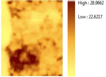
4.1 Land Surface Temperature
Land Surface Temperature in degrees Celsius was derived from the Landsat 8 image. It is seen in the resulting image that the lower left area has generally higher temperatures than the rest of the image.
Figure 2. 2014 Land Surface Temperature image
Statistics from the LST image were also calculated and can be
Table 3. Statistics of the Land Surface Temperature image 4.2 Land Use Land Cover Classification
The LiDAR and orthophoto data was successfully classified with an accuracy of not less than 90% overall accuracy and 85% Kappa coefficient. The resulting classes were agricultural fields, bare land, built-up, grassland, roads, trees, and water.
Figure 3. Land Use Land Cover Classification image with corresponding legend
The study area is composed of 44.15% of agricultural fields, 17.15% of trees, 15.26% of grassland, 10.66% of water, 6.19% of builtup, 3.94% of bare land, and 2.65% of roads according to the results. It is observable that the lower left area of the image is highly urbanized as it is mostly classified as either built-up and roads. This corresponds to the same area in the LST image where the concentration of high temperatures is.
4.3 Statistical Analysis of Data
There are 10,990 cases with 73 spatial metrics as predictors of surface temperature. Approximately, 16.22% (12 out of 73) of the spatial metrics have incomplete data while approximately 83.78% (61 out 73) of the spatial metrics have complete data. Out of 813,260 values the data has, approximately 8.736% is missing as seen in Figure 4.
Figure 4. Distribution of complete and incomplete data in the variables, cases and values.
Using the Little‟s MCAR Test, missing values were identified as missing randomly or non-randomly. Since p-value is less than 0.05, which means that it is not significant, we can conclude that the values are missing not at random (MNAR).
Figure 5. Result of Little‟s MCAR test. Circled in red shows the significance to be .000 which shows the data to be MNAR. Upon knowing that the missing data is MNAR, Expectation Maximization was done to treat the data. After treating all the missing values the data was checked if it satisfied the assumptions of multiple linear regression. It appeared that more than one assumption was not met, which may result to incorrect or misleading analysis. Some of the predictor variables were not included in the analysis to solve this problem. These predictor variables were the ones which do not pose high importance in predicting the response variable: land surface temperature. Table 4 shows which of the remaining assumptions (1, 2, 3, 7) are satisfied or not satisfied by each class.
Table 4. Summary of which classes satisfy each assumption After checking the preliminary output, the following variables were included in the analysis:
Landscape shape index
Fractal index distribution (median) Contiguity index distribution (median) Perimeter-area fractal dimension Proximity index distribution Percentage of like adjacencies
As
Interspersion and juxtaposition index Effective mesh size
Splitting index Aggregation index
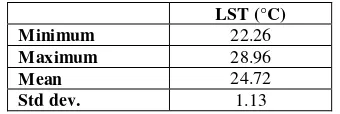
Including the said variables in the analysis would still violate the assumption that residuals are independent. This could be due to bias that is explainable by omitted variables. Therefore, we just ignore this violation. After doing Multi Linear Regression, the top predictors per class were determined. Using these top predictors, a linear model for each class was then created to predict LST. Table 5 shows the top predictors as well as the linear model created per class.
Table 5. Summary of all classes with their top predictors and linear models for LST
It was found that except for the class Road, all other classes have Effective mesh size as one of their top predictors or their only top predictor. If it is not the only predictor, it still has the biggest weight among the other variables in the linear regression models in each class. This means that Effective mesh size is a very important variable of Land Use Land Cover Classification in predicting LST. Effective mesh size is calculated by the following equation (Jaeger, 2000):
∑
Where = area ( of patch ij A = total landscape area (
The advantage of utilizing effective mesh size in the model is that it is „area-proportionately additive‟ which means that it characterizes the subdivision of a landscape independently of its size (Jaeger, 2000).
5. CONCLUSION AND RECOMMENDATION
Land Surface Temperature was derived from a Landsat 8 image although it was not validated due to equipment limitations. LULC classification was also derived from LiDAR and Orthophoto data. The LULC classification resulted in 7 classes namely agricultural fields, bare land, built-up, road, trees, and water. Class-level spatial metrics were derived from the LULC classification. After statistical analysis of the class-level spatial metrics and their relationship with LST, it was found that the spatial metric “Effective mesh size” was the most common variable in predicting LST as it appeared as a top predictor for 6 out of 7 classes, with Road as the only class without “Effective mesh size” as a top predictor.
The thermal data used to derive LST was acquired during a specific period (just before the end of the growing season). This has an effect on the LST since the crops are at the peak of their growth which would imply that the area would generally have lower temperatures. Analysis of the LST of another farming period would provide a better analysis of the relationship between LST and LULC landscape patterns. Aside from checking if effective mesh size remains a predictor for LST for an LST in a different farming period, finding the common predictors for two LSTs from different farming periods will give a more generalized model for predicting LST. With a generalized prediction model of LST based on LULC, better urban planning can be done with respect to the predicted LST to reduce heat-related stress and ailments in the area.
6. ACKNOWLEDGEMENTS
The authors would like to acknowledge the Department of Science and Technology (DOST) of the Philippines as the funding agency and the Department of Science and Technology – Philippine Council for Industry, Energy and Emerging Technology Research and Development as the monitoring agency.
7. REFERENCES
Artis, D. A., Carnahan, W. H., 1982. Survey of emissivity variability in thermography of urban areas. Remote Sensing of Environment 12, pp. 313-329.
Land Cover
Bare Land Effective mesh size,
Carlson, T. N., Ripley D. A., 1997. On the relation between NDVI fractional vegetation cover, and leaf area index. Remote Sensing of Environment 62, pp. 241-252.
Dempster, A. P., Laird, N. M., Rubin D. B., 1977. Maximum Likelihood from Incomplete Data via the EM Algorithm.
Journal of the Royal Statistical Society. Series B (Methodological) 39, pp. 1-38.
Garson, G. D., 2015. Missing Values Analysis and Data Imputation 2015 edition, Statistical Associates Blue Book Series, p. 12.
Jaeger, J. A. G., 2000. Landscape Division, Splitting Index, and Effective Mesh Size: New Measures of Landscape Fragmentation. Landscape Ecology 15, pp, 115-130.
Little, R. J. A., 1988. A Test of Missing Completely at Random for Multivariate Data with Missing Values. Journal of the American Statistical Association 83, pp. 1198-1202.
Markham, B. L., Barker, J. L., 1985. Special Issue: LIDQA Final Symposium. Photogrammetric Engineering and Remote Sensing 51, pp. 1245-1493.
McGarigal, K., Cushman, S.A., Ene, E., 2012. “FRAGSTATS V4: Spatial Pattern Analysis Program for Categorical and Continuous Maps.” Computer Software Program Produced by the Authors at the University of Massachusetts, Amherst. http://www.umass.edu/landeco/research/fragstats/fragstats.html Montgomery, D., Peck, E., Vining, G., 2012. Introduction to Linear Regression Analysis 5th Edition, Wiley.
Rinner, C., Hussain, M., 2011. Toronto‟s Urban Heat Island – Exploring the Relationship between Land Use and Surface Temperature. Remote Sens 3, pp. 1251-1265.
Sobrino, J., Jiménez-Muñoz, J., Paolini, L., 2004. Land Surface Temperature retrieval from LANDSAT TM 5. Remote Sensing of Environment 90, pp. 434-440.
Sundara Kumar, K., Udaya Bhaskar P., Padmakumari, K., 2012. Estimation of Land Surface Temperature to Study Urban Heat Island Effect Using Landsat ETM+ Image. International Journal of Engineering Science and Technology 4, pp. 771-778. Trimble, 2014. eCognition Developer Reference Book, pp. 32-39.
U.S. Geological Survey, 2015. Landsat 8 (L8) Data Users Handbook.
http://landsat.usgs.gov/documents/Landsat8DataUsersHandboo k.pdf (3 Dec. 2015).
Weng, Q., Lu, D., Schubring, J., 2004. Estimation of land surface temperature – vegetation abundance relationship for urban heat island studies. Remote Sensing of Environment 89, pp. 467-483.
Yu, X., Guo, X., Wu, Z., 2014. Land Surface Temperature Retrieval from Landsat 8 TIRS – Comparison between Radiative Transfer Equation-Based Method, Split Window Algorithm and Single Channel Method. Remote Sens 6, pp. 9829-9852.