This chapter continues our analysis of the forces governing long-run economic growth.With the basic version of the Solow growth model as our starting point, we take on four new tasks.
Our first task is to make the Solow model more general and more realistic. In Chapter 3 we saw that capital, labor, and technology are the key determinants of a nation’s production of goods and services. In Chapter 7 we developed the Solow model to show how changes in capital (saving and investment) and changes in the labor force (population growth) affect the economy’s output. We are now ready to add the third source of growth—changes in technology—into the mix.
Our second task is to examine how a nation’s public policies can influence the level and growth of its standard of living. In particular, we address four questions: Should our society save more or save less? How can policy influence the rate of saving? Are there some types of investment that policy should especially encour-age? How can policy increase the rate of technological progress? The Solow growth model provides the theoretical framework within which we consider each of these policy issues.
Our third task is to move from theory to empirics.That is, we consider how well the Solow model fits the facts. During the 1990s, a large literature examined the predictions of the Solow model and other models of economic growth. It turns out that the glass is both half full and half empty. The Solow model can shed much light on international growth experiences, but it is far from the last word on the subject.
Our fourth and final task is to consider what the Solow model leaves out. As we have discussed previously, models help us understand the world by simplifying it. After completing an analysis of a model, therefore, it is important to consider
| 207
8
Economic Growth II
C H A P T E RIs there some action a government of India could take that would lead the
Indian economy to grow like Indonesia’s or Egypt’s? If so, what, exactly? If
not, what is it about the “nature of India” that makes it so? The
conse-quences for human welfare involved in questions like these are simply
stag-gering: Once one starts to think about them, it is hard to think about
anything else.
whether we have oversimplified matters. In the last section, we examine a new set of theories, called endogenous growth theories, that hope to explain the technological progress that the Solow model takes as exogenous.
8-1
Technological Progress in
the Solow Model
So far, our presentation of the Solow model has assumed an unchanging rela-tionship between the inputs of capital and labor and the output of goods and ser-vices. Yet the model can be modified to include exogenous technological progress, which over time expands society’s ability to produce.
The Efficiency of Labor
To incorporate technological progress, we must return to the production func-tion that relates total capital Kand total labor Lto total output Y. Thus far, the production function has been
Y=F(K,L).
We now write the production function as
Y=F(K,L×E),
where E is a new (and somewhat abstract) variable called the efficiency of labor.The efficiency of labor is meant to reflect society’s knowledge about pro-duction methods: as the available technology improves, the efficiency of labor rises. For instance, the efficiency of labor rose when assembly-line production transformed manufacturing in the early twentieth century, and it rose again when computerization was introduced in the the late twentieth century. The ef-ficiency of labor also rises when there are improvements in the health, education, or skills of the labor force.
The term L×Emeasures the number of effective workers. It takes into account the number of workers Land the efficiency of each worker E.This new produc-tion funcproduc-tion states that total output Ydepends on the number of units of capital Kand on the number of effective workers L×E. Increases in the efficiency of labor Eare, in effect, like increases in the labor force L.
The Steady State With Technological Progress
Expressing technological progress as labor augmenting makes it analogous to population growth. In Chapter 7 we analyzed the economy in terms of quanti-ties per worker and allowed the number of workers to rise over time. Now we analyze the economy in terms of quantities per effective worker and allow the number of effective workers to rise.
To do this, we need to reconsider our notation. We now let k= K/(L × E) stand for capital per effective worker and y=Y/(L×E) stand for output per ef-fective worker.With these definitions, we can again write y=f(k).
This notation is not really as new as it seems. If we hold the efficiency of labor Econstant at the arbitrary value of 1, as we have done implicitly up to now, then these new definitions of kand yreduce to our old ones.When the efficiency of labor is growing, however, we must keep in mind that kand ynow refer to quan-tities per effective worker (not per actual worker).
Our analysis of the economy proceeds just as it did when we examined popu-lation growth.The equation showing the evolution of kover time now changes to
D
k=sf(k) −(d
+n+g)k.As before, the change in the capital stock
D
k equals investment sf(k) minus break-even investment (d
+ n+ g)k. Now, however, because k = K/EL, break-even investment includes three terms: to keep kconstant,d
kis needed to replace depreciating capital,nk is needed to provide capital for new workers, and gkis needed to provide capital for the new “effective workers”created by technologi-cal progress.As shown in Figure 8-1, the inclusion of technological progress does not sub-stantially alter our analysis of the steady state. There is one level of k, denoted
f i g u r e 8 - 1
Investment, break-even investment
k*, at which capital per effective worker and output per effective worker are constant. As before, this steady state represents the long-run equilibrium of the economy.
The Effects of Technological Progress
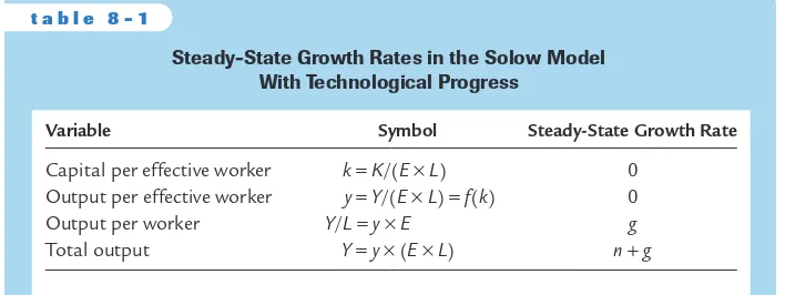
Table 8-1 shows how four key variables behave in the steady state with technolog-ical progress. As we have just seen, capital per effective worker kis constant in the steady state. Because y=f(k), output per effective worker is also constant. Remem-ber, though, that the efficiency of each actual worker is growing at rate g. Hence, output per worker (Y/L=y×E) also grows at rate g.Total output [Y=y×(E×L)] grows at rate n+g.
With the addition of technological progress, our model can finally explain the sustained increases in standards of living that we observe.That is, we have shown that technological progress can lead to sustained growth in output per worker. By contrast, a high rate of saving leads to a high rate of growth only until the steady state is reached. Once the economy is in steady state, the rate of growth of output per worker depends only on the rate of technological progress.According to the Solow model, only technological progress can explain persistently rising living standards.
The introduction of technological progress also modifies the criterion for the Golden Rule.The Golden Rule level of capital is now defined as the steady state that maximizes consumption per effective worker. Following the same argu-ments that we have used before, we can show that steady-state consumption per effective worker is
c*=f(k*) −(
d
+n+g)k*.Steady-state consumption is maximized if
MPK=
d
+n+g,or
MPK−
d
=n+g.That is, at the Golden Rule level of capital, the net marginal product of capital, MPK −
d
, equals the rate of growth of total output, n + g. Because actualVariable Symbol Steady-State Growth Rate
Capital per effective worker k =K/(E×L) 0 Output per effective worker y =Y/(E×L) =f(k) 0 Output per worker Y/L=y×E g
Total output Y=y×(E×L) n+g Steady-State Growth Rates in the Solow Model
economies experience both population growth and technological progress, we must use this criterion to evaluate whether they have more or less capital than at the Golden Rule steady state.
8-2
Policies to Promote Growth
Having used the Solow model to uncover the relationships among the different sources of economic growth, we can now use the theory to help guide our thinking about economic policy.
Evaluating the Rate of Saving
According to the Solow growth model, how much a nation saves and invests is a key determinant of its citizens’standard of living. So let’s begin our policy discus-sion with a natural question: Is the rate of saving in the U.S. economy too low, too high, or about right?
As we have seen, the saving rate determines the steady-state levels of capital and output. One particular saving rate produces the Golden Rule steady state, which maximizes consumption per worker and thus economic well-being.The Golden Rule provides the benchmark against which we can compare the U.S. economy.
To decide whether the U.S. economy is at, above, or below the Golden Rule steady state, we need to compare the marginal product of capital net of deprecia-tion (MPK −
d
) with the growth rate of total output (n+ g). As we just estab-lished, at the Golden Rule steady state,MPK −d
= n + g. If the economy is operating with less capital than in the Golden Rule steady state, then diminish-ing marginal product tells us that MPK −d
>n+ g. In this case, increasing the rate of saving will eventually lead to a steady state with higher consumption. However, if the economy is operating with too much capital, then MPK−d
<n+g, and the rate of saving should be reduced.
To make this comparison for a real economy, such as the U.S. economy, we need an estimate of the growth rate (n+ g) and an estimate of the net marginal product of capital (MPK −
d
). Real GDP in the United States grows an average of 3 percent per year, so n+g =0.03.We can estimate the net marginal product of capital from the following three facts:1. The capital stock is about 2.5 times one year’s GDP.
2. Depreciation of capital is about 10 percent of GDP.
3. Capital income is about 30 percent of GDP.
Using the notation of our model (and the result from Chapter 3 that capital owners earn income of MPKfor each unit of capital), we can write these facts as
1.k=2.5y.
2.
d
k=0.1y.We solve for the rate of depreciation
d
by dividing equation 2 by equation 1:d
k/k=(0.1y)/(2.5y)d
=0.04.And we solve for the marginal product of capital MPKby dividing equation 3 by equation 1:
(MPK×k)/k=(0.3y)/(2.5y) MPK=0.12
Thus, about 4 percent of the capital stock depreciates each year, and the marginal product of capital is about 12 percent per year.The net marginal product of cap-ital,MPK−
d
, is about 8 percent per year.We can now see that the return to capital (MPK−
d
=8 percent per year) is well in excess of the economy’s average growth rate (n+g=3 percent per year). This fact, together with our previous analysis, indicates that the capital stock in the U.S. economy is well below the Golden Rule level. In other words, if the United States saved and invested a higher fraction of its income, it would grow more rapidly and eventually reach a steady state with higher consumption. This finding suggests that policymakers should want to increase the rate of saving and investment. In fact, for many years, increasing capital formation has been a high priority of economic policy.Changing the Rate of Saving
The preceding calculations show that to move the U.S. economy toward the Golden Rule steady state, policymakers should increase national saving. But how can they do that? We saw in Chapter 3 that, as a matter of sheer accounting, higher national saving means higher public saving, higher private saving, or some combination of the two. Much of the debate over policies to increase growth centers on which of these options is likely to be most effective.
The most direct way in which the government affects national saving is through public saving—the difference between what the government receives in tax revenue and what it spends.When the government’s spending exceeds its rev-enue, the government is said to run a budget deficit, which represents negative public saving. As we saw in Chapter 3, a budget deficit raises interest rates and crowds out investment; the resulting reduction in the capital stock is part of the burden of the national debt on future generations. Conversely, if the government spends less than it raises in revenue, it is said to run a budget surplus. It can then re-tire some of the national debt and stimulate investment.
rate of return that savers earn. However, tax-exempt retirement accounts, such as IRAs, are designed to encourage private saving by giving preferential treatment to income saved in these accounts.
Many disagreements among economists over public policy are rooted in dif-ferent views about how much private saving responds to incentives. For example, suppose that the government were to expand the amount that people could put into tax-exempt retirement accounts.Would people respond to the increased in-centive to save by saving more? Or would people merely transfer saving done in other forms into these accounts—reducing tax revenue and thus public saving without any stimulus to private saving? Clearly, the desirability of the policy de-pends on the answers to these questions. Unfortunately, despite much research on this issue, no consensus has emerged.
C A S E S T U D Y
Should the Social Security System Be Reformed?
Although many government policies are designed to encourage saving, such as the preferential tax treatment given to pension plans and other retirement ac-counts, one important policy is often thought to reduce saving: the Social Secu-rity system. Social SecuSecu-rity is a transfer system designed to maintain individuals’
income in their old age.These transfers to the elderly are financed with a payroll tax on the working-age population.This system is thought to reduce private sav-ing because it reduces individuals’need to provide for their own retirement.
To counteract the reduction in national saving attributed to Social Security, many economists have proposed reforms of the Social Security system.The sys-tem is now largely pay-as-you-go: most of the current tax receipts are paid out to the current elderly population. One suggestion is that Social Security should be
fully funded. Under this plan, the government would put aside in a trust fund the payments a generation makes when it is young and working; the government would then pay out the principal and accumulated interest to this same genera-tion when it is older and retired. Under a fully funded Social Security system, an increase in public saving would offset the reduction in private saving.
These issues rose to prominence in the late 1990s as policymakers became aware that the current Social Security system was not sustainable. That is, the amount of revenue being raised by the payroll tax appeared insufficient to pay all the benefits being promised. According to most projections, this problem was to become acute as the large baby-boom generation retired during the early decades of the twenty-first century.Various solutions were proposed. One possi-bility was to maintain the current system with some combination of smaller ben-efits and higher taxes. Other possibilities included movements toward a fully funded system, perhaps also including private accounts.This issue was prominent in the presidential campaign of 2000, with candidate George W. Bush advocating a reform including private accounts. As this book was going to press, it was still unclear whether this reform would come to pass.1
1To learn more about the debate over Social Security, see Social Security Reform: Links to Saving,
In-vestment, and Growth, Steven A. Sass and Robert K. Triest, eds., Conference Series No. 41, Federal Reserve Bank of Boston, June 1997.
2N. Gregory Mankiw, David Romer, and David N.Weil,“A Contribution to the Empirics of
Eco-nomic Growth,’’Quarterly Journal of Economics(May 1992): 407–437.
Allocating the Economy’s Investment
The Solow model makes the simplifying assumption that there is only one type of capital. In the world, of course, there are many types. Private businesses invest in traditional types of capital, such as bulldozers and steel plants, and newer types of capital, such as computers and robots.The government invests in various forms of public capital, called infrastructure, such as roads, bridges, and sewer systems.
In addition, there is human capital—the knowledge and skills that workers acquire through education, from early childhood programs such as Head Start to on-the-job training for adults in the labor force.Although the basic Solow model includes only physical capital and does not try to explain the efficiency of labor, in many ways human capital is analogous to physical capital. Like physical capital, human capital raises our ability to produce goods and services. Raising the level of human capital requires investment in the form of teachers, libraries, and student time. Recent re-search on economic growth has emphasized that human capital is at least as impor-tant as physical capital in explaining international differences in standards of living.2
Other economists have suggested that the government should actively encour-age particular forms of capital. Suppose, for instance, that technological advance occurs as a by-product of certain economic activities.This would happen if new and improved production processes are devised during the process of building capital (a phenomenon called learning by doing) and if these ideas become part of society’s pool of knowledge. Such a by-product is called a technological externality (or a knowledge spillover). In the presence of such externalities, the social returns to capital exceed the private returns, and the benefits of increased capital accumula-tion to society are greater than the Solow model suggests.3Moreover, some types of capital accumulation may yield greater externalities than others. If, for example, installing robots yields greater technological externalities than building a new steel mill, then perhaps the government should use the tax laws to encourage in-vestment in robots.The success of such an industrial policy, as it is sometimes called, requires that the government be able to measure the externalities of different eco-nomic activities so it can give the correct incentive to each activity.
Most economists are skeptical about industrial policies, for two reasons. First, measuring the externalities from different sectors is so difficult as to be virtually impossible. If policy is based on poor measurements, its effects might be close to random and, thus, worse than no policy at all. Second, the political process is far from perfect. Once the government gets in the business of rewarding specific in-dustries with subsidies and tax breaks, the rewards are as likely to be based on po-litical clout as on the magnitude of externalties.
One type of capital that necessarily involves the government is public capital. Local, state, and federal governments are always deciding whether to borrow to finance new roads, bridges, and transit systems. During his first presidential cam-paign, Bill Clinton argued that the United States had been investing too little in infrastructure. He claimed that a higher level of infrastructure investment would make the economy substantially more productive. Among economists, this claim had both defenders and critics.Yet all of them agree that measuring the marginal product of public capital is difficult. Private capital generates an easily measured rate of profit for the firm owning the capital, whereas the benefits of public cap-ital are more diffuse.
Encouraging Technological Progress
The Solow model shows that sustained growth in income per worker must come from technological progress. The Solow model, however, takes technological progress as exogenous; it does not explain it. Unfortunately, the determinants of technological progress are not well understood.
Despite this limited understanding, many public policies are designed to stim-ulate technological progress. Most of these policies encourage the private sector to devote resources to technological innovation. For example, the patent system
3
Paul Romer,“Crazy Explanations for the Productivity Slowdown,’’NBER Macroeconomics Annual
gives a temporary monopoly to inventors of new products; the tax code offers tax breaks for firms engaging in research and development; and government agencies such as the National Science Foundation directly subsidize basic re-search in universities. In addition, as discussed above, proponents of industrial policy argue that the government should take a more active role in promoting specific industries that are key for rapid technological progress.
C A S E S T U D Y
The Worldwide Slowdown in Economic Growth
Beginning in the early 1970s, world policymakers faced a perplexing problem—
a global slowdown in economic growth.Table 8-2 presents data on the growth in real GDP per person for the seven major world economies. Growth in the United States fell from 2.2 percent to 1.5 percent, and other countries experi-enced similar or more severe declines.Accumulated over many years, even a small change in the rate of growth has a large effect on economic well-being. Real in-come in the United States today is about 20 percent lower than it would have been had growth remained at its previous level.
Why did this slowdown occur? Studies have shown that it was attributable to a fall in the rate at which the production function was improving over time. The appendix to this chapter explains how economists measure changes in the pro-duction function with a variable called total factor productivity, which is closely re-lated to the efficiency of labor in the Solow model. There are, however, many hypotheses to explain this fall in productivity growth. Here are four of them.
Measurement Problems One possibility is that the productivity slowdown did not really occur and that it shows up in the data because the data are flawed. As you may recall from Chapter 2, one problem in measuring inflation is correcting for changes in the quality of goods and services.The same issue arises when mea-suring output and productivity. For instance, if technological advance leads to
morecomputers being built, then the increase in output and productivity is easy to measure. But if technological advance leads to faster computers being built, then output and productivity have increased, but that increase is more subtle and harder to measure. Government statisticians try to correct for changes in quality, but despite their best efforts, the resulting data are far from perfect.
Unmeasured quality improvements mean that our standard of living is rising more rapidly than the official data indicate.This issue should make us suspicious of the data, but by itself it cannot explain the productivity slowdown.To explain a slow-downin growth, one must argue that the measurement problems got worse.There is some indication that this might be so.As history passes, fewer people work in indus-tries with tangible and easily measured output, such as agriculture, and more work in industries with intangible and less easily measured output, such as medical ser-vices.Yet few economists believe that measurement problems were the full story.
this explanation has appeared less likely. One reason is that the accumulated short-fall in productivity seems too large to be explained by an increase in oil prices—oil is not that large a fraction of the typical firm’s costs. In addition, if this explanation were right, productivity should have sped up when political turmoil in OPEC caused oil prices to plummet in 1986. Unfortunately, that did not happen.
Worker Quality Some economists suggest that the productivity slowdown
might have been caused by changes in the labor force. In the early 1970s, the large baby-boom generation started leaving school and taking jobs. At the same time, changing social norms encouraged many women to leave full-time house-work and enter the labor force. Both of these developments lowered the average level of experience among workers, which in turn lowered average productivity.
Other economists point to changes in worker quality as gauged by human capital. Although the educational attainment of the labor force continued to rise throughout this period, it was not increasing as rapidly as it did in the past. More-over, declining performance on some standardized tests suggests that the quality of education was declining. If so, this could explain slowing productivity growth.
The Depletion of Ideas Still other economists suggest that the world started to
run out of new ideas about how to produce in the early 1970s, pushing the econ-omy into an age of slower technological progress.These economists often argue that the anomaly is not the period since 1970 but the preceding two decades. In the late 1940s, the economy had a large backlog of ideas that had not been fully imple-mented because of the Great Depression of the 1930s and World War II in the first half of 1940s. After the economy used up this backlog, the argument goes, a slow-down in productivity growth was likely. Indeed, although the growth rates in the 1970s, 1980s, and early 1990s were disappointing compared to those of the 1950s and 1960s, they were not lower than average growth rates from 1870 to 1950.
GROWTH IN OUTPUT PER PERSON (PERCENT PER YEAR)
Country 1948–1972 1972–1995 1995–2000
Canada 2.9 1.8 2.7
France 4.3 1.6 2.2
West Germany 5.7 2.0
Germany 1.7
Italy 4.9 2.3 4.7
Japan 8.2 2.6 1.1
United Kingdom 2.4 1.8 2.5
United States 2.2 1.5 2.9
Source: Angus Maddison, Phases of Capitalist Development(Oxford: Oxford University Press, 1982); and OECD National Accounts and International Financial Statistics.
Note:Data before 1995 for Germany refer to West Germany; after 1995, to the unified Germany.
The Slowdown in Growth Around the World
4
For various views on the growth slowdown, see “Symposium: The Slowdown in Productivity Growth,’’The Journal of Economic Perspectives2 (Fall 1988): 3–98.
Which of these suspects is the culprit? All of them are plausible, but it is difficult to prove beyond a reasonable doubt that any one of them is guilty.The worldwide slowdown in economic growth that began in the mid-1970s remains a mystery.4
C A S E S T U D Y
Information Technology and the New Economy
As any good doctor will tell you, sometimes a patient’s illness goes away on its own, even if the doctor has failed to come up with a convincing diagnosis and remedy.This seems to be the outcome with the productivity slowdown discussed in the previous case study. Economists have not yet figured it out, but beginning in the middle of the 1990s, the problem disappeared. Economic growth took off, as shown in the third column of Table 8-2. In the United States, output per per-son accelerated from 1.5 to 2.9 percent per year. Commentators proclaimed we were living in a “new economy.”
As with the slowdown in economic growth in the 1970s, the acceleration in the 1990s is hard to explain definitively. But part of the credit goes to advances in computer and information technology, including the Internet.
Observers of the computer industry often cite Moore’s law, which states that the price of computing power falls by half every 18 months. This is not an in-evitable law of nature but an empirical regularity describing the rapid technolog-ical progress this industry has enjoyed. In the 1980s and early 1990s, economists were surprised that the rapid progress in computing did not have a larger effect on the overall economy. Economist Robert Solow once quipped that “we can see the computer age everywhere but in the productivity statistics.”
There are two reasons why the macroeconomic effects of the computer revo-lution might not have showed up until the mid-1990s. One is that the computer industry was previously only a small part of the economy. In 1990, computer hardware and software represented 0.9 percent of real GDP; by 1999, this share had risen to 4.2 percent. As computers made up a larger part of the economy, technological advance in that sector had a greater overall effect.
The second reason why the productivity benefits of computers may have been delayed is that it took time for firms to figure out how best to use the technol-ogy.Whenever firms change their production systems and train workers to use a technology, they disrupt the existing means of production. Measured productiv-ity can fall for a while before the economy reaps the benefits. Indeed, some economists even suggest that the spread of computers can help explain the pro-ductivity slowdown that began in the 1970s.
re-place steam engines with electric motors; they had to rethink the entire organi-zation of factories. Similarly, replacing the typewriters on desks with computers and word processing programs, as was common in the 1980s, may have had small productivity effects. Only later, when the Internet and other advanced applica-tions were invented, did the computers yield large economic gains.
Eventually, advances in technology should show up in economic growth, as was the case in the second half of the 1990s. This extra growth occurs through three channels. First, because the computer industry is part of the economy, pro-ductivity growth in that industry directly affects overall propro-ductivity growth. Second, because computers are a type of capital good, falling computer prices allow firms to accumulate more computing capital for every dollar of investment spending; the resulting increase in capital accumulation raises growth in all sec-tors that use computers as a factor of production. Third, the innovations in the computer industry may induce other industries to reconsider their own produc-tion methods, which in turn leads to productivity growth in those industries.
The big, open question is whether the computer industry will remain an en-gine of growth. Will Moore’s law describe the future as well as it has described the past? Will the technological advances of the next decade be as profound as the Internet was during the 1990s? Stay tuned.5
5For more on this topic, see the symposium on “Computers and Productivity”in the Fall 2000 issue of The Journal of Economic Perspectives. On the parallel between electricity and computers, see Paul A. David,“The Dynamo and the Computer:A Historical Perspective on the Modern Produc-tivity Paradox,”American Economic Review80, no. 2 (May 1990): 355–361.
8-3
From Growth Theory to Growth Empirics
So far in this chapter we have introduced exogenous technological progress into the Solow model to explain sustained growth in standards of living.We then used the theoretical framework as a lens through which to view some key issues facing policymakers. Let’s now discuss what happens when the theory is asked to con-front the facts.
Balanced Growth
According to the Solow model, technological progress causes the values of many variables to rise together in the steady state.This property, called balanced growth, does a good job of describing the long-run data for the U.S. economy.
Technological progress also affects factor prices. Problem 3(d) at the end of the chapter asks you to show that, in the steady state, the real wage grows at the rate of technological progress. The real rental price of capital, however, is constant over time.Again, these predictions hold true for the United States. Over the past 50 years, the real wage has increased about 2 percent per year; it has increased about the same amount as real GDP per worker.Yet the real rental price of capital (measured as real capital income divided by the capital stock) has remained about the same.
The Solow model’s prediction about factor prices—and the success of this prediction—is especially noteworthy when contrasted with Karl Marx’s theory of the development of capitalist economies. Marx predicted that the return to capital would decline over time and that this would lead to economic and polit-ical crises. Economic history has not supported Marx’s prediction, which partly explains why we now study Solow’s theory of growth rather than Marx’s.
Convergence
If you travel around the world, you will see tremendous variations in living stan-dards. The world’s poor countries have average levels of income per person that are less than one-tenth the average levels in the world’s rich countries.These dif-ferences in income are reflected in almost every measure of the quality of life—
from the number of televisions and telephones per household to the infant mortality rate and life expectancy.
Much research has been devoted to the question of whether economies con-verge over time to one another. In particular, do economies that start off poor subsequently grow faster than economies that start off rich? If they do, then the world’s poor economies will tend to catch up with the world’s rich economies. This property of catch-up is called convergence.
To understand the study of convergence, consider an analogy. Imagine that you were to collect data on college students. At the end of their first year, some students have A averages, whereas others have C averages.Would you expect the A and the C students to converge over the remaining three years of college? The answer depends on why their first-year grades differed. If the differences arose because some students came from better high schools than others, then you might expect those who were initially disadvantaged to start catching up to their better-prepared peers. But if the differences arose because some students study more than others, you might expect the differences in grades to persist.
Experience is consistent with this analysis. In samples of economies with sim-ilar cultures and policies, studies find that economies converge to one another at a rate of about 2 percent per year. That is, the gap between rich and poor economies closes by about 2 percent each year. An example is the economies of individual American states. For historical reasons, such as the Civil War of the 1860s, income levels varied greatly among states a century ago.Yet these differ-ences have slowly disappeared over time.
In international data, a more complex picture emerges.When researchers ex-amine only data on income per person, they find little evidence of convergence: countries that start off poor do not grow faster on average than countries that start off rich. This finding suggests that different countries have different steady states. If statistical techniques are used to control for some of the determinants of the steady state, such as saving rates, population growth rates, and educational at-tainment, then once again the data show convergence at a rate of about 2 percent per year. In other words, the economies of the world exhibit conditional conver-gence: they appear to be converging to their own steady states, which in turn are determined by saving, population growth, and education.6
Factor Accumulation Versus Production Efficiency
As a matter of accounting, international differences in income per person can be attributed to either (1) differences in the factors of production, such as the quan-tities of physical and human capital, or (2) differences in the efficiency with which economies use their factors of production. That is, a worker in a poor country may be poor because he lacks tools and skills or because the tools and skills he has are not being put to their best use.To describe this issue in terms of the Solow model, the question is whether the large gap between rich and poor is explained by differences in capital accumulation (including human capital) or differences in the production function.
Much research has attempted to estimate the relative importance of these two sources of income disparities. The exact answer varies from study to study, but both factor accumulation and production efficiency appear important. More-over, a common finding is that they are positively correlated: nations with high levels of physical and human capital also tend to use those factors efficiently.7
There are several ways to interpret this positive correlation. One hypothesis is that an efficient economy may encourage capital accumulation. For example, a person in a well-functioning economy may have greater resources and incentive
6
Robert Barro and Xavier Sala-i-Martin,“Convergence Across States and Regions,”Brookings Pa-pers on Economic Activity, no. 1 (1991): 107–182; and N. Gregory Mankiw, David Romer, and David N. Weil,“A Contribution to the Empirics of Economic Growth,”Quarterly Journal of Economics
(May 1992): 407–437.
7
to stay in school and accumulate human capital.Another hypothesis is that capital accumulation may induce greater efficiency. If there are positive externalities to physical and human capital, a possibility mentioned earlier in the chapter, then countries that save and invest more will appear to have better production func-tions (unless the research study accounts for these externalities, which is hard to do).Thus, greater production efficiency may cause greater factor accumulation, or the other way around.
A final hypothesis is that both factor accumulation and production efficiency are driven by a common third variable. Perhaps the common third variable is the quality of the nation’s institutions, including the government’s policymaking process.As one economist put it, when governments screw up, they screw up big time. Bad policies, such as high inflation, excessive budget deficits, widespread market interference, and rampant corruption, often go hand in hand.We should not be surprised that such economies both accumulate less capital and fail to use the capital they have as efficiently as they might.
8-4
Beyond the Solow Model:
Endogenous Growth Theory
A chemist, a physicist, and an economist are all trapped on a desert island, trying to figure out how to open a can of food.
“Let’s heat the can over the fire until it explodes,”says the chemist.
“No, no,”says the physicist,“Let’s drop the can onto the rocks from the top of a high tree.”
“I have an idea,”says the economist.“First, we assume a can opener . . . .”
This old joke takes aim at how economists use assumptions to simplify—and sometimes oversimplify—the problems they face. It is particularly apt when eval-uating the theory of economic growth. One goal of growth theory is to explain the persistent rise in living standards that we observe in most parts of the world. The Solow growth model shows that such persistent growth must come from technological progress. But where does technological progress come from? In the Solow model, it is simply assumed!
To understand fully the process of economic growth, we need to go beyond the Solow model and develop models that explain technological progress. Mod-els that do this often go by the label endogenous growth theory, because they reject the Solow model’s assumption of exogenous technological change. Al-though the field of endogenous growth theory is large and sometimes complex, here we get a quick sampling of this modern research.8
8
The Basic Model
To illustrate the idea behind endogenous growth theory, let’s start with a particu-larly simple production function:
Y=AK,
where Y is output,K is the capital stock, and A is a constant measuring the amount of output produced for each unit of capital. Notice that this production function does not exhibit the property of diminishing returns to capital. One extra unit of capital produces Aextra units of output, regardless of how much capital there is.This absence of diminishing returns to capital is the key difference between this endogenous growth model and the Solow model.
Now let’s see how this production function relates to economic growth. As before, we assume a fraction sof income is saved and invested.We therefore de-scribe capital accumulation with an equation similar to those we used previously:
D
K=sY−d
K.This equation states that the change in the capital stock (∆K) equals investment (sY) minus depreciation (
d
K). Combining this equation with the Y= AK pro-duction function, we obtain, after a bit of manipulation,D
Y/Y=D
K/K=sA−d
.This equation shows what determines the growth rate of output
D
Y/Y. Notice that, as long as sA>d
, the economy’s income grows forever, even without the as-sumption of exogenous technological progress.Thus, a simple change in the production function can alter dramatically the predictions about economic growth. In the Solow model, saving leads to growth temporarily, but diminishing returns to capital eventually force the economy to approach a steady state in which growth depends only on exogenous technolog-ical progress. By contrast, in this endogenous growth model, saving and invest-ment can lead to persistent growth.
But is it reasonable to abandon the assumption of diminishing returns to cap-ital? The answer depends on how we interpret the variable Kin the production function Y=AK. If we take the traditional view that Kincludes only the econ-omy’s stock of plants and equipment, then it is natural to assume diminishing re-turns. Giving 10 computers to each worker does not make the worker 10 times as productive as he or she is with one computer.
returns to knowledge.) If we accept the view that knowledge is a type of capital, then this endogenous growth model with its assumption of constant returns to capital becomes a more plausible description of long-run economic growth.
A Two-Sector Model
Although the Y=AKmodel is the simplest example of endogenous growth, the
theory has gone well beyond this. One line of research has tried to develop mod-els with more than one sector of production in order to offer a better description of the forces that govern technological progress. To see what we might learn from such models, let’s sketch out an example.
The economy has two sectors, which we can call manufacturing firms and re-search universities. Firms produce goods and services, which are used for con-sumption and investment in physical capital. Universities produce a factor of production called “knowledge,”which is then freely used in both sectors. The economy is described by the production function for firms, the production func-tion for universities, and the capital-accumulafunc-tion equafunc-tion:
Y=F[K,(1 −u)EL] (production function in manufacturing firms),
D
E=g(u)E (production function in research universities),D
K=sY−d
K (capital accumulation),where uis the fraction of the labor force in universities (and 1 - uis the fraction in manufacturing),E is the stock of knowledge (which in turn determines the efficiency of labor), and g is a function that shows how the growth in knowl-edge depends on the fraction of the labor force in universities. The rest of the notation is standard. As usual, the production function for the manufacturing firms is assumed to have constant returns to scale: if we double both the amount of physical capital (K) and the number of effective workers in manufacturing [(1 −u)EL], we double the output of goods and services (Y).
This model is a cousin of the Y=AK model. Most important, this economy
exhibits constant (rather than diminishing) returns to capital, as long as capital is broadly defined to include knowledge. In particular, if we double both physical capital Kand knowledge E, then we double the output of both sectors in the economy. As a result, like the Y=AK model, this model can generate persistent
growth without the assumption of exogenous shifts in the production function. Here persistent growth arises endogenously because the creation of knowledge in universities never slows down.
There are two key decision variables in this model.As in the Solow model, the
fraction of output used for saving and investment,s, determines the steady-state
stock of physical capital. In addition, the fraction of labor in universities,u,
deter-mines the growth in the stock of knowledge. Both sand uaffect the level of
in-come, although only uaffects the steady-state growth rate of income. Thus, this
model of endogenous growth takes a small step in the direction of showing which societal decisions determine the rate of technological change.
The Microeconomics of Research and Development
The two-sector endogenous growth model just presented takes us closer to un-derstanding technological progress, but it still tells only a rudimentary story about the creation of knowledge. If one thinks about the process of research and development for even a moment, three facts become apparent. First, although knowledge is largely a public good (that is, a good freely available to everyone),
much research is done in firms that are driven by the profit motive. Second,
re-search is profitable because innovations give firms temporary monopolies, either
because of the patent system or because there is an advantage to being the first
firm on the market with a new product. Third, when one firm innovates, other
firms build on that innovation to produce the next generation of innovations.
These (essentially microeconomic) facts are not easily connected with the (es-sentially macroeconomic) growth models we have discussed so far.
Some endogenous growth models try to incorporate these facts about re-search and development. Doing this requires modeling the decisions that firms face as they engage in research and modeling the interactions among firms that have some degree of monopoly power over their innovations. Going into more detail about these models is beyond the scope of this book. But it should be clear already that one virtue of these endogenous growth models is that they offer a more complete description of the process of tech-nological innovation.
One question these models are designed to address is whether, from the
standpoint of society as a whole, private profit-maximizing firms tend to engage
in too little or too much research. In other words, is the social return to research (which is what society cares about) greater or smaller than the private return
(which is what motivates individual firms)? It turns out that, as a theoretical
matter, there are effects in both directions. On the one hand, when a firm
cre-ates a new technology, it makes other firms better off by giving them a base of
knowledge on which to build future research. As Isaac Newton famously
re-marked,“If I have seen farther than others, it is because I was standing on the
shoulders of giants.”On the other hand, when one firm invests in research, it
can also make other firms worse off by merely being first to discover a
technol-ogy that another firm would have invented. This duplication of research effort
has been called the “stepping on toes”effect. Whether firms left to their own
devices do too little or too much research depends on whether the positive
“standing on shoulders”externality or the negative “stepping on toes”
Although theory alone is ambiguous about the optimality of research effort, the empirical work in this area is usually less so. Many studies have suggested the
“standing on shoulders”externality is important and, as a result, the social return to research is large—often in excess of 40 percent per year.This is an impressive rate of return, especially when compared to the return to physical capital, which we earlier estimated to be about 8 percent per year. In the judgment of some economists, this finding justifies substantial government subsidies to research.9
8-5
Conclusion
Long-run economic growth is the single most important determinant of the economic well-being of a nation’s citizens. Everything else that macroeconomists study—unemployment, inflation, trade deficits, and so on—pales in comparison. Fortunately, economists know quite a lot about the forces that govern eco-nomic growth. The Solow growth model and the more recent endogenous growth models show how saving, population growth, and technological progress interact in determining the level and growth of a nation’s standard of living. Al-though these theories offer no magic pill to ensure an economy achieves rapid growth, they do offer much insight, and they provide the intellectual framework for much of the debate over public policy.
Summary
1.In the steady state of the Solow growth model, the growth rate of income per
person is determined solely by the exogenous rate of technological progress.
2.In the Solow model with population growth and technological progress, the
Golden Rule (consumption-maximizing) steady state is characterized by equality between the net marginal product of capital (MPK −
d
) and the steady-state growth rate (n + g). By contrast, in the U.S. economy, the net marginal product of capital is well in excess of the growth rate, indicating that the U.S. economy has much less capital than in the Golden Rule steady state.3.Policymakers in the United States and other countries often claim that their
nations should devote a larger percentage of their output to saving and in-vestment. Increased public saving and tax incentives for private saving are two ways to encourage capital accumulation.
4.In the early 1970s, the rate of growth fell substantially in most industrialized
countries. The cause of this slowdown is not well understood. In the mid-1990s, the rate of growth increased, most likely because of advances in infor-mation technology.
9For an overview of the empirical literature on the effects of research, see Zvi Griliches,“The