123
SPRING ER BRIEFS IN ELEC TRIC AL AND CO MPUTER
ENG INEER ING
CONTROL, AUTOMATION AND ROBOTICS
Simona Onori
Lorenzo Serrao
Giorgio Rizzoni
Hybrid Electric
Vehicles
Energy
Engineering
Control, Automation and Robotics
Giorgio Rizzoni
Hybrid Electric Vehicles
Energy Management Strategies
Simona Onori
Automotive Engineering Department Clemson University
Greenville, SC USA
Lorenzo Serrao
Dana Mechatronics Technology Center Dana Holding Corporation
Rovereto Italy
Giorgio Rizzoni
Department of Mechanical and Aerospace Engineering and Center for Automotive Research
The Ohio State University Columbus, OH
USA
ISSN 2191-8112 ISSN 2191-8120 (electronic)
SpringerBriefs in Electrical and Computer Engineering
ISSN 2192-6786 ISSN 2192-6794 (electronic)
SpringerBriefs in Control, Automation and Robotics
ISBN 978-1-4471-6779-2 ISBN 978-1-4471-6781-5 (eBook) DOI 10.1007/978-1-4471-6781-5
Library of Congress Control Number: 2015952754
Springer London Heidelberg New York Dordrecht ©The Author(s) 2016
This work is subject to copyright. All rights are reserved by the Publisher, whether the whole or part of the material is concerned, specifically the rights of translation, reprinting, reuse of illustrations, recitation, broadcasting, reproduction on microfilms or in any other physical way, and transmission or information storage and retrieval, electronic adaptation, computer software, or by similar or dissimilar methodology now known or hereafter developed.
The use of general descriptive names, registered names, trademarks, service marks, etc. in this publication does not imply, even in the absence of a specific statement, that such names are exempt from the relevant protective laws and regulations and therefore free for general use.
The publisher, the authors and the editors are safe to assume that the advice and information in this book are believed to be true and accurate at the date of publication. Neither the publisher nor the authors or the editors give a warranty, express or implied, with respect to the material contained herein or for any errors or omissions that may have been made.
Printed on acid-free paper
—
Simona Onori
To my parents, Salvatore and Silvana
—
Lorenzo Serrao
To my family
Preface
The origin of hybrid electric vehicles dates back to 1899, when Dr. Ferdinand Porsche, then a young engineer at Jacob Lohner & Co, built thefirst hybrid vehicle [1], the Lohner-Porsche gasoline-electric Mixte. After Porsche, other inventors proposed hybrid vehicles in the early twentieth century, but then the internal combustion engine technology improved significantly and hybrid vehicles, much like battery-electric vehicles, disappeared from the market for a long time.
Nearly a century later, hybrid powertrain concepts returned strongly, in the form of many research prototypes but also as successful commercial products: Toyota launched the Prius—the first purpose-designed and -built hybrid electric vehicle—in 1998, and Honda launched the Insight in 1999. What made the new generation of hybrid vehicles more successful than their ancestors was the com-pletely new technology now available, especially in terms of electronics and control systems to coordinate and exploit at best the complex subsystems interacting in a hybrid vehicle. Substantial support to research in this field was provided by gov-ernment initiatives, such as the USPartnership for a New Generation of Vehicles
(PNGV) [2], which involved DaimlerChrysler, Ford Motor Company, and General Motors Corporation. PNGV provided the opportunity for many research projects to be carried out in collaborations among the automotive companies, their suppliers, national laboratories, and universities. The material assembled in this book is an outgrowth of the experience that the authors gained while working together at the Ohio State University Center for Automotive Research, one of the PNGV academic labs, which has been engaged in programs focused on the development of vehicle prototypes and on the development of energy management strategies and algo-rithms since 1995.
Energy management strategies are necessary to achieve the full potential of hybrid electric vehicles, which can reduce fuel consumption and emissions in comparison to conventional vehicles, thanks to the presence of a reversible energy storage device and one or more electric machines. The presence of an additional energy storage device gives rise to new degrees of freedom, which in turn translate into the need of finding the most efficient way of splitting the power demand
between the engine and the battery. The energy management strategy is the control layer to which this task is demanded.
Despite many articles on hybrid electric vehicles system, control, and opti-mization, there has not been a book that systematically discusses deeper aspects of the model-based design of energy management strategies. Thus, the aim of this book is to present a systematic model-based approach and propose a formal framework to cast the energy management problem using optimal control theory tools and language.
The text focuses on the development of model-based supervisory controller when the fuel consumption is being minimized. It does not consider other cost functions, such as pollutant emissions or battery aging. Drivability issues such as noise, harshness, and vibrations are neglected as well as heuristic supervisory controllers design.
The aim is to provide an adequate presentation to meet the ever-increasing demand for engineers to look for rigorous methods for hybrid electric vehicles analysis and design.
We hope that this book will be suitable to educate mechanical and electrical engineering graduate students, professional engineers, and practitioners on the topic of hybrid electric vehicle control and optimization.
Acknowledgments
We are extremely grateful to all our colleagues for the fruitful discussions on the topics discussed in this book. We are also grateful to Springer editorial staff for their support and patience.
August 2015 Simona Onori
Lorenzo Serrao Giorgio Rizzoni
References
1. Hybrid cars. (Online). Availablehttp://www.hybridcars.com/history/history-of-hybrid-vehicles. html
Contents
1 Introduction. . . 1
1.1 Hybrid Electric Vehicles . . . 1
1.2 HEV Architectures . . . 2
1.3 Energy Analysis of Hybrid Electric Vehicles . . . 4
1.4 Book Structure. . . 5
References . . . 6
2 HEV Modeling. . . 7
2.1 Introduction. . . 7
2.2 Modeling for Energy Analysis . . . 7
2.3 Vehicle-Level Energy Analysis . . . 8
2.3.1 Equations of Motion. . . 8
2.3.2 Forward and Backward Modeling Approaches . . . 10
2.3.3 Vehicle Energy Balance . . . 13
2.3.4 Driving Cycles . . . 15
2.4 Powertrain Components . . . 18
2.4.1 Internal Combustion Engine . . . 18
2.4.2 Torque Converter. . . 19
2.4.3 Gear Ratios and Mechanical Gearbox . . . 20
2.4.4 Planetary Gear Sets . . . 22
2.4.5 Wheels, Brakes, and Tires. . . 23
2.4.6 Electric Machines . . . 25
2.4.7 Batteries . . . 25
2.4.8 Engine Accessories and Auxiliary Loads. . . 29
References . . . 30
3 The Energy Management Problem in HEVs . . . 31
3.1 Introduction. . . 31
3.2 Energy Management of Hybrid Electric Vehicles . . . 31
3.3 Classification of Energy Management Strategies. . . 33
3.4 The Optimal Control Problem in Hybrid Electric Vehicles. . . 34
3.4.1 Problem Formulation . . . 35
3.4.2 General Problem Formulation . . . 37
References . . . 39
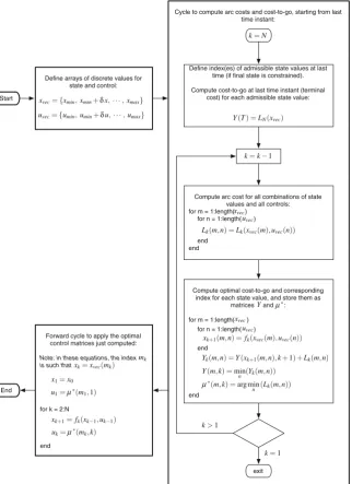
4 Dynamic Programming. . . 41
4.1 Introduction. . . 41
4.2 General Formulation . . . 41
4.3 Application of DP to the Energy Management Problem in HEVs . . . 43
4.3.1 Implementation Example. . . 46
References . . . 49
5 Pontryagin’s Minimum Principle. . . 51
5.1 Introduction. . . 51
5.2 Minimum Principle for Problems with Constraints on the State . . . 52
5.2.1 On the System State Boundaries . . . 53
5.2.2 Notes on the Minimum Principle . . . 54
5.3 Pontryagin’s Minimum Principle for the Energy Management Problem in HEVs. . . 55
5.3.1 Power-Based PMP Formulation . . . 58
5.4 Co-Stateλand Cost-to-Go Function . . . 60
References . . . 63
6 Equivalent Consumption Minimization Strategy . . . 65
6.1 Introduction. . . 65
6.2 ECMS-Based Supervisory Control . . . 65
6.3 Equivalence Between Pontryagin's Minimum Principle and ECMS . . . 71
6.4 Correction of Fuel Consumption to Account for SOC Variation . . . 72
6.5 Historical Note: One of the First Examples of ECMS Implementation . . . 74
References . . . 76
7 Adaptive Optimal Supervisory Control Methods . . . 79
7.1 Introduction. . . 79
7.2 Review of Adaptive Supervisory Control Methods . . . 80
7.2.1 Adaptation Based on Driving Cycle Prediction . . . 80
7.2.2 Adaptation Based on Driving Pattern Recognition . . . 82
7.3 Adaptation Based on Feedback from SOC. . . 82
7.3.1 Analysis and Comparison of A-PMP Methods . . . 83
7.3.2 Calibration of Adaptive Strategies . . . 84
8 Case Studies . . . 89
8.1 Introduction. . . 89
8.2 Parallel Architecture . . . 89
8.2.1 Powertrain Model . . . 89
8.2.2 Optimal Control Problem Solution . . . 92
8.2.3 Model Implementation . . . 95
8.2.4 Simulation Results . . . 98
8.3 Power-Split Architecture . . . 101
8.3.1 Powertrain Model . . . 101
8.3.2 Optimal Control Problem Solution . . . 105
8.3.3 Model Implementation . . . 105
8.3.4 Simulation Results . . . 106
References . . . 109
Series Editors’Biographies . . . 111
t Time
t0 Initial time of the optimization horizon
tf Final time of the optimization horizon
xðtÞ State of the optimal control problem
xðtÞ State vector,xðtÞ 2Rn
uðtÞ Scalar control of the optimal control problem
uðtÞ Control vector,uðtÞ 2Rp
(Relative to the optimal solution)
aveh Vehicle acceleration
Af Frontal area of the vehicle
a Distance of CG from front axle
b Distance of CG from rear axle
Cd Coefficient of aerodynamic drag
croll Rolling resistance coefficient
crr0 Rolling resistance model coefficient (constant term)
crr1 Rolling resistance model coefficient (speed-dependent term)
C Electrical capacitance
Eaero Energy dissipated in aerodynamic resistance
Ebatt Battery energy
Ekin Kinetic energy
Epot Potential energy
Epwt Energy delivered at the wheels by the powertrain
Eroll Energy dissipated in rolling resistance
Faero Aerodynamic resistance
Fgrade Grade force (due to slope)
Finertia Inertial force
Froll Rolling resistance
Ftrac Total tractive force at the wheel-road interface
gfd Gear ratio (final drive)
gfb Gear ratio (generic follower/base ratio)
gtr Gear ratio (transmission)
Gðx;tÞ State constraints
hCG Height of the center of gravity
HðÞ Hamiltonian function
itr Gear index (transmission)
I Current
J Cost function of optimal control problem
Ktc Capacity factor (in torque converter)
k Time index in discrete-time problems
L Instantaneous cost of optimal control problem _
melec Instantaneous virtual fuel consumption corresponding to the use of electrical power
_
meqv Instantaneous equivalent fuel consumption
_
mf Instantaneous fuel consumption (fuel massflow rate)
mf Total fuel consumption (fuel mass)
Mveh Vehicle mass
MR Multiplication ratio or torque ratio (in torque converter)
N Number of elements
Pacc Mechanical power for secondary accessories
Pgen;e Electrical power at the generator
Pgen;m Mechanical power at the generator
Peng Mechanical power generated by the internal combustion engine
Ppto Mechanical power for PTO (power take-off) accessories
Preq Total power request by the driver
Ptrac Total tractive power at the wheel
Qnom Nominal charge capacity (of a battery)
Qlhv Fuel lower heating value
R0 Electrical resistance
RPM Rotational speed expressed in revolutions per minute
SR Speed ratio (in torque converter)
Tb Base shaft torque (in generic gear set)
Tbrake Brake torque at the wheel
Tc Carrier torque (in planetary gear set)
Tevt Torque at the output of EVT transmission
Teng Internal combustion engine torque
Tem Electric machine torque
Tf Follower shaft torque (in generic gear set)
Tgen Electric generator torque
Tmot Electric motor torque
Tpwt Powertrain torque at the wheel
Tp Pump (impeller) torque (in torque converter)
Tr Ring torque (in planetary gear set)
Ts Sun torque (in planetary gear set)
Tt Turbine torque (in torque converter)
Ttrac Total tractive torque at the wheel
U Admissible control set
VL Load voltage at the battery terminals
Voc Open circuit voltage
vveh Vehicle speed
Y Cost to go
BMS Battery Management System
BSFC Brake specific fuel consumption
CG Center of gravity
DP Dynamic Programming
ICE Internal combustion engine PMP Pontryagin’s Minimum Principle RESS Rechargeable energy storage system
SOC State of charge
α Accelerator pedal position (normalized) β Brake pedal position (normalized)
δ Road grade
η Efficiency
λ Co-state variable
µ Optimal control matrix in dynamic programming ν Friction coefficient
ωb Base shaft speed (in generic gear set) ωc Carrier speed (in planetary gear set) ωevt Speed at the output of EVT transmission ωeng Internal combustion engine speed ωem Electric machine speed
ωb Follower shaft speed (in generic gear set) ωgen Electric generator speed
ωmot Electric motor speed
ωp Pump (impeller) speed (in torque converter) ωr Ring speed (in planetary gear set)
ωs Sun speed (in planetary gear set) ωt Turbine speed (in torque converter)
ωwh Wheel speed
Ωx Set of admissible states
φðxf;tfÞ Terminal cost of optimal control problem
π Control policy (in dynamic programming)
ρ Planetary gear ratio
ρair Air density
θ Temperature
Chapter 1
Introduction
1.1
Hybrid Electric Vehicles
Hybrid vehicles are so defined because their propulsion systems are equipped with two energy sources, complementing each other: a high-capacity storage (typically a chemical fuel in liquid or gaseous form), and a lower capacity rechargeable energy storage system (RESS) that can serve as an energy storage buffer, but also as a means for recovering vehicle kinetic energy or to provide power assist. The RESS can be electrochemical (batteries or supercapacitors), hydraulic/pneumatic (accumulators) or mechanical (flywheel) [1]. This dual energy storage capability, in which the RESS permits bi-directional power flows, requires that at least two energy converters be present, at least one of which must also have the ability to allow for bi-directional power flows.Hybrid electricvehicles (HEVs), which represent the majority of hybrid vehicles on the road today, use electrochemical batteries as the RESS, and electric machines (one or more) as secondary energy converters, while a reciprocating internal combustion engine (ICE), fueled by a hydrocarbon fuel, serves as the primary energy converter. A fuel cell or other types of combustion engine (gas turbine, external combustion engines) could also serve as the primary energy converter.
The RESS can be used for regenerative braking and also acts as an energy buffer for the primary energy converter, e.g., an ICE, which can instantaneously deliver an amount of power different than what is required by the vehicle load. This flexibility in engine management results in the ability to operate the engine more often in conditions where it is more efficient or less polluting [2, 3]. Other benefits offered by hybridization are the possibility to shut down the engine when it is not needed (such as at a stop or at low speed), and the downsizing of the engine: since the peak power can be reached by summing the output from the engine and from the RESS, the former can be downsized, i.e. replaced with a smaller and less powerful engine, operating at higher average efficiency.Plug-inhybrid electric vehicles (PHEVs) allow battery recharge from the electric grid and offer a significant range in pure electric mode. The details of what can actually be accomplished depend on the architecture of the propulsion system and of the vehicle powertrain, as described in the next section.
© The Author(s) 2016
S. Onori et al.,Hybrid Electric Vehicles, SpringerBriefs in Control, Automation and Robotics, DOI 10.1007/978-1-4471-6781-5_1
1.2
HEV Architectures
The powertrain of a conventional vehicle is composed by an internal combustion engine, driving the wheels through a transmission that realizes a variable speed ratio between the engine speed and the wheel speed. A dry clutch or hydrodynamic torque converter interposed between engine and transmission decouples the engine from the wheels when needed, i.e., during the transients in which the transmission speed ratio is being modified. All the torque propelling the vehicle is produced by the engine or the mechanical brakes, and there is a univocal relation between the torque at the wheels and the torque developed by the engine (positive) or the brakes (negative).
Hybrid electric vehicles, on the other hand, include one or more electric machines coupled to the engine and/or the wheels [4]. A possible classification of today’s vehicles in the market can be given based on internal combustion engine size and electric machine size as shown in Fig.1.1[5] and detailed in the following:
1. Conventional ICE vehicles; 2. Micro hybrids (start/stop);
3. Mild hybrids (start/stop+kinetic energy recovery+engine assist); 4. Full hybrids (mild hybrid capabilities+electric launch);
5. Plug-in hybrids (full hybrid capabilities+electric range); 6. Electric Vehicles (battery or fuel cell).
Differences and main characteristics of the different types of vehicles are outlined below [2,6–8].
Size of Internal
Comb
u
stion En
g
ine
Size of Electric Motor and Battery 1. Conventional Vehicle
(ICE only)
2. Micro Hybrids
(start/stop)
3. Mild Hybrids
(start/stop + kinetic energy recovery)
4. Full Hybrids
(mild hybrid + electric launch + engine assist)
5. Plug-in Hybrids
(full hybrid + electric range)
6. Electric vehicles
(battery or fuel cell)
1.2 HEV Architectures 3
1. In conventional vehicles the ICE is the only source of power. For this type of vehicles the total power request at the wheel is entirely satisfied by the ICE. 2. Start–stop systems allow the ICE to shut down and restart to reduce the amount of
time spent idling, thus reducing fuel consumption and emissions. This solution is very advantageous for vehicles which spend significant amounts of time waiting at traffic lights or frequently come to a stop in traffic. This feature is present in hybrid electric vehicles, but has also appeared in vehicles which lack a hybrid electric powertrain. Nonelectric vehicles featuring start–stop systems are called micro hybrids.
3. In mild hybrid vehicles generally the ICE is coupled with an electric machine (one motor/generator in a parallel configuration) allowing the engine to be turned off whenever the car is coasting, braking, or stopping. Mild hybrids can also employ regenerative breaking and some level of ICE power assist, but do not have an exclusive electric-only mode of propulsion.
4. Full hybrid electric vehicles run on just the engine, just the battery, or a combi-nation of both. A high-capacity battery pack is needed for battery-only operation during the electric launch. Differently from micro and mild hybrids, where simple heuristic rules are typically used to coordinate the ICE start–stop and power assist functionality, in full hybrid vehicles energy management strategies are needed to fully exploit the benefits of vehicle hybridization, by providing coordination among the actuators in order to minimize fuel consumption.
5. Plug-in hybrid electric vehicles are hybrid vehicles utilizing rechargeable batteries that can be restored to full charge by connecting them to an external electric power source. PHEVs share the characteristics of both full hybrid electric vehicles, having electric motor and an ICE, and of all-electric vehicles, having a plug to connect to the electrical grid.
6. Electric vehicles are propelled only by their on-board electric motor(s), which are powered by a battery (recharged from the power grid) or a hydrogen fuel cell.
In this book, we focus on full hybrid electric vehicles. The number and position of the machines present in full hybrid vehicles define the powertrain architecture, and therefore the performance and capabilities of the hybrid vehicles themselves. HEV architectures can be classified as follows [8]:
• series: the engine drives a generator, producing electrical power which can be summed to the electrical power coming from the RESS and then transmitted, via an electric bus, to the electric motor(s) driving the wheels;
• parallel: the power summation is mechanical rather than electrical: the engine and the electric machines (one or more) are connected with a gear set, a chain, or a belt, so that their torque is summed and then transmitted to the wheels;
• series/parallel: the engagement/disengagement of one or two clutches allows to change the powertrain configuration from series to parallel and vice versa, thus allowing the use of the configuration best suited to the current operating conditions.
The series architecture has the advantage of requiring only electrical connections between the main power conversion devices. This simplifies some aspects of vehicle packaging and design. Also, having the engine completely disconnected from the wheels gives great freedom in choosing its load and speed, thus making it possible for the engine to operate at the highest possible efficiency. On the other hand, series hybrids require two energy conversions (mechanical to electrical in the generator, and electrical to mechanical in the motor), which introduce losses, even in cases when a direct mechanical connection of the engine to the wheels would actually be more efficient, overall. For this reason, there are conditions in which a series hybrid vehicle consumes more fuel than its conventional counterpart: for example, in highway driving. Further, one of the two electromechanical energy converters must be sized to support the maximum power requirements of the vehicle, since it is the primary source of motive power. The parallel architecture does not have this problem; however, unless significantly oversized, the electric motors are less powerful than those used in a series hybrid (because not all the mechanical power flows through them), thus reducing the potential for regenerative braking; also, the engine operating conditions cannot be determined as freely as in a series hybrid architecture, because the engine speed is mechanically related (via the transmission) to the vehicle velocity. Power split and series/parallel architectures (which can be realized in different ways) are the most flexible, and give a higher degree of control of the operating conditions of the engine than the parallel architecture while applying the double energy conversion typical of series operation only to a fraction of the total power flow, thus reducing overall losses [3,8].
1.3
Energy Analysis of Hybrid Electric Vehicles
1.3 Energy Analysis of Hybrid Electric Vehicles 5
path). The ratio of the power flows generated by each path constitutes an additional degree of freedom that permits optimization of the engine operating conditions to achieve improvements in efficiency and fuel economy. In addition, the electric motors are reversible and can produce negative torque. Thus, they can replace or supplement the mechanical brakes as a means to decelerate the vehicle, with the benefit of acting like generators and producing electrical energy, which can be stored in batteries on board of the vehicle for later use. This operation, known asregenerative braking, may substantially improve the overall efficiency over an extended time period. The additional freedom afforded by a hybrid architecture makes the use of a power man-agement strategy necessary, both over a short time horizon, to recover braking energy and to guarantee performance and instantaneous fuel economy, as well as over a long time horizon, to guarantee that the RESS has sufficient energy in store when needed, and that fuel economy benefits are achieved. Hence, the need for anenergy man-agementstrategy arises, which extends the power management (instantaneous) with considerations based on a longer time horizon, keeping into account the amount of energy stored in the vehicle.
The energy management strategy determines at each instant the power reparti-tion between the engine and the RESS, according to instantaneous constraints (e.g., generating the total power output requested by the driver), global constraints (e.g., maintaining the RESS energy level within safety limits) and global objectives (e.g., minimizing the fuel consumption during a trip).
1.4
Book Structure
References
1. W. Liu,Introduction to Hybrid Vehicle System Modeling and Control(Wiley, Hoboken, 2013) 2. L. Guzzella, A. Sciarretta,Vehicle Propulsion Systems: Introduction to Modeling and
Optimiza-tion(Springer, Berlin, 2013)
3. G. Rizzoni, H. Peng, Hybrid and electric vehicles: the role of dynamics and control. ASME Dyn. Syst. Control Mag.1(1), 10–17 (2013)
4. C.C. Chan, The state of the art of electric and hybrid vehicles. Proc. IEEE90(2), 245–275 (2002) 5. A.A. Pesaran, Choices and requirements of batteries for EVs, HEVs, PHEVs, in
NREL/PR-5400-51474 (2011)
6. F. An, F. Stodolsky, D. Santini, Hybrid options for light-duty vehicles, in SAE Technical Paper No. 1999-01-2929 (1999)
7. F. An, A. Vyas, J. Anderson, D. Santini, Evaluating commercial and prototype HEVs, in SAE Technical Paper No. 2001-01-0951 (2001)
Chapter 2
HEV Modeling
2.1
Introduction
The objective of the energy management control is to minimize the vehicle fuel consumption, while maintaining the battery state of charge around a desired value. To this end, modeling for energy management may have two scopes: creating plant simulators to which an energy management strategy is applied for testing and devel-opment, or creating embedded models that are used to set up analytically and/or solve numerically the energy management problem. Plant models tend to be more accurate and computationally heavy than embedded control models. The main objective in both cases is to reproduce the energy flows within the powertrain and the vehicle, in order to obtain an accurate estimation of fuel consumption and battery state of charge, based on the control inputs and the road load. In some applications, other quantities may be of interest, such as thermal flows (temperature variation in engine, batteries, after-treatment, etc.), battery aging, pollutant emissions, etc.
This chapter provides a concise overview of the modeling issues linked to the development and simulation of energy management strategies. The reader is referred to more specialized works for further details (e.g., [1]). Efficiency considerations are at the basis of the models described, which are suited for preliminary analysis and high-level energy management development.
2.2
Modeling for Energy Analysis
Because of the losses in the powertrain, the net amount of energy produced at the wheels is smaller than the amount of energy introduced into the vehicle from external sources (e.g., fuel). Conversion losses take place when power is transformed into a different form (e.g., chemical into mechanical, mechanical into electrical, etc.). Similarly, when power flows through a connection device, friction losses and other inefficiencies reduce the amount of power at the device output. Energy losses in powertrain components are usually modeled using efficiency maps, i.e., tables that contain efficiency data as a function of the operating conditions (for example, the output torque and the rotational speed of the engine). Maps are built experimentally
© The Author(s) 2016
S. Onori et al.,Hybrid Electric Vehicles, SpringerBriefs in Control, Automation and Robotics, DOI 10.1007/978-1-4471-6781-5_2
as a set of stationary points, i.e., letting the component reach a steady-state operating condition and measuring power input and output (and/or power dissipation) in that condition. Because of this procedure, efficiency maps may not be accurate during transients. Despite this, the approach is widely used because it allows to generate simple models capable of being evaluated quickly when implemented in computer code, and validation results [2] show that the accuracy of such models can be very good for estimating fuel consumption and energy balance, as most of the energy content is associated with the slower system dynamics [3].
The vehicle fuel consumption for a prescribed driving cycle can be estimated using abackwardor aforwardmodeling approach. The backward, quasi-static approach is based on the assumption that the prescribed driving cycle is followed exactly by the vehicle. The driving cycle is subdivided in small time intervals, during which an average operating point approach is applied, assuming that speed, torque, and accel-eration remain constant: this is equivalent to neglecting internal powertrain dynamics and taking average values of all variables during the selected sampling time, which is therefore longer than typical powertrain transients (e.g., engine dynamics, gear shifting), and of the same order of magnitude of vehicle longitudinal dynamics and driving cycle variations. Each powertrain component is modeled using an efficiency map, a power loss map, or a fuel consumption map: these give a relation between the losses in the component and the present operating conditions (averaged during the desired time interval).
The forward, dynamic approach is based on a first-principles description of each powertrain component, with dynamic equations describing the evolution of its state. The degree of modeling detail depends on the timescale and the nature of the phe-nomena that the model should predict. In the simplest case, the same level of detail as the quasi-static approach can be applied, but the evolution of vehicle speed is computed as the result of the dynamic simulation and not prescribed a priori.
2.3
Vehicle-Level Energy Analysis
By vehicle-level energy analysis, we refer to the case in which the vehicle is consid-ered as a point mass and its interaction with the external environment is studied, in order to compute the amount of power and energy needed to move it with specified speed. This high-level approach is useful to develop an understanding of the vehicle longitudinal dynamics and of the energy characteristics of hybrid vehicles.
2.3.1
Equations of Motion
2.3 Vehicle-Level Energy Analysis 9
Froll
Ftrac
Faero
Fgrade
Mvehg
δ
Finertia
Fig. 2.1 Forces acting on a vehicle
Mveh
dvveh
dt =Finertia=Ftrac−Froll−Faero−Fgrade, (2.1)
where Mveh is the effective vehicle mass,vvehis the longitudinal vehicle velocity,
Finertiais the inertial force,Ftrac=Fpwt−Fbrakeis the tractive force generated by the
powertrain and the brakes at the wheels,1Frollis the rolling resistance (friction due
to tire deformation and losses),Faerothe aerodynamic resistance,Fgradethe force due
to road slope.
The aerodynamic resistance is expressed as
Faero=
1
2ρairAfCdv
2
veh, (2.2)
whereρairis the air density (1.25 kg/m3in normal conditions),Afthe vehicle frontal
area,Cdthe aerodynamic drag coefficient.
The rolling resistance force is usually modeled as [1]
Froll=croll(vveh,ptire, . . .)Mvehg cosδ, (2.3)
where g is the gravity acceleration,δthe road slope angle (so thatMvehg cosδis the
vertical component of the vehicle weight), andcrollis a rolling resistance coefficient
which is, in principle, a function of vehicle speed, tire pressureptire, external
temper-ature, etc. In most cases,crollis assumed to be constant, or to be an affine function
of the vehicle speed:
croll=cr0+cr1vveh. (2.4)
Table 2.1 Typical values of vehicle-dependent parameters for longitudinal vehicle dynamics mod-els
Parameter Compact car Full-size car SUV
Mveh 1200–1500 kg 1700–2000 kg 1900–2200 kg
Cd 0.3–0.35 0.28–0.33 0.32–0.38
Af 1.3–1.7 m2 1.8–2.2 m2 2–2.5 m2
croll 0.01–0.03 0.01–0.03 0.01–0.03
The order of magnitude of croll is 0.01–0.03 (for a light vehicle on normal road
surface), which means that the rolling resistance is 1–3 % of the vehicle weight (depending on vehicle, soil, tires and tire pressure, temperature, etc.).
The grade force is the horizontal component of the vehicle weight, which opposes (or facilitates) vehicle motion only if the vehicle is moving uphill (or downhill):
Fgrade=Mvehg sinδ. (2.5)
These basic equations represent the starting point for vehicle modeling, and can be sufficiently accurate if the parameters are correctly identified. Typical values of the vehicle-level parameters are listed in Table2.1.
2.3.2
Forward and Backward Modeling Approaches
Equation (2.1) can be rearranged to calculate the tractive force that the powertrain needs to produce, given the acceleration (inertial forceFinertia):
Ftrac=Fpwt−Fbrake=Finertia+Fgrade+Froll+Faero. (2.6)
The different form of (2.1) and (2.6) corresponds to the forward and backward modeling approaches: in (2.1), the vehicle accelerationdvveh
dt is computed as a
2.3 Vehicle-Level Energy Analysis 11
Driving cycle
Driver model
Drivetrain Wheel dynamicsVehicle Speed
Fig. 2.2 Information flow in a forward simulator
The forward approach is the option typically chosen in most simulators; it is char-acterized by the information flow as shown in Fig.2.2. For example, in the case of a hybrid vehicle forward simulator, the desired speed (from the cycle inputs) is com-pared to the actual vehicle speed, and braking or throttle commands are generated using a driver model (e.g., a PID speed controller) in order to follow the imposed vehi-cle profile. This driver command is an input to the supervisor block that is responsible of issuing the actuators setpoints (engine, electric machines, and braking torques) to the rest of the powertrain components, which ultimately produce a tractive force. Finally, the force is applied to the vehicle dynamics model, where the acceleration is determined with (2.1), taking into account the road load information [5].
In a backward simulator, instead (see Fig.2.3), no driver model is necessary, since the desired speed is a direct input to the simulator, while the engine torque and fuel consumption are outputs. The simulator determines the net tractive force to be applied based on the velocity, payload, and grade profiles, along with the vehi-cle characteristics. Based on this information, the torque that the powertrain should apply is calculated, and then the torque/speed characteristics of the various power-train components are taken into account in order to determine the engine operating conditions and, finally, the fuel consumption.
Driving
Both the forward and backward simulation approaches have their relative strengths and weaknesses. Fuel economy simulations are typically conducted over predeter-mined driving cycles, and therefore using a backward simulator ensures that each different simulation exactly follows this profile, which guarantees consistency of simulation results. By contrast, a forward simulator may not exactly follow the trace, as it introduces a small error between the actual and the desired signal. Proper tuning of the driver block can reduce the differences, whereas the backward version keeps the error at zero without any effort. On the other hand, a backward simulation assumes that the vehicle and powertrain are capable of following the speed trace, and does not account for limitations of the powertrain actuators in computing the vehicle speed, which is predetermined. This poses the problem of evaluating demanding cycles which may require more power than the powertrain can provide. A forward simula-tion does not have this issue, because the speed is computed from the torque/force output, which can be saturated according to the powertrain limitations. For this rea-son, forward simulation can also be used for acceleration tests and in general for testing the behavior of the system at saturation. In addition, forward simulators are implemented according to physical causality and, if their level of detail is appro-priate, can be used for development of online control strategies, while a backward simulator is suited for preliminary screening of energy management strategies. It is possible to combine the advantages of both modeling approaches, i.e., the accurate reproduction of a cycle by a backward simulation and the ability to capture power-train limitations of a forward simulator. A solution, represented in Fig.2.4, consists in using a forward simulator in which the driver model (speed controller) uses a backward vehicle model to compute the torque setpoints to be applied: in this way, the resulting speed profile will match exactly the reference cycle, if this does not
Driver model
2.3 Vehicle-Level Energy Analysis 13
saturate the powertrain capacity, but will be appropriately saturated when needed since it goes through a forward powertrain model. A feedback term should also be added, in order to recover speed deviation due to powertrain saturation (or to possible mismatches between the backward and forward models).
2.3.3
Vehicle Energy Balance
Fuel consumption evaluation is conducted by analyzing the energy flows in the powertrain and identifying the areas in which saving can be introduced. From (2.6) the inertial force Finertia is positive when the vehicle is accelerating, and negative
during deceleration; the grade force Fgrade is positive when the vehicle is driven
uphill and negative when it is going downhill; the rolling (Froll) and aerodynamic
(Faero) resistances are always positive (for a vehicle moving in forward direction).
The forcesFrollandFaeroare dissipative, since they always oppose the motion of
the vehicle, while the inertial and grade forces are conservative, being only depen-dent on the vehicle state (respectively velocity and altitude). Thus, part of the tractive force generated by the powertrain increases the kinetic and potential energy of the vehicle (by accelerating it and moving it uphill), and part is dissipated in rolling and aerodynamic resistances. When the vehicle decelerates or drives downhill, its potential and kinetic energy must be dissipated: rolling and aerodynamic resistances contribute to dissipating part of the vehicle energy, but for faster deceleration the mechanical brakes must be used. Thus, ultimately, all the energy that the powertrain produces is dissipated in these three forms: rolling resistance, aerodynamic resis-tance, and mechanical brakes. The net variation of kinetic energy is always zero between two stops (since initial speed and final speed are both zero), and the varia-tion of potential energy only depends on the difference of altitude between the initial and ending point of the trip considered.
Multiplying all terms of (2.6) by the vehicle speed (vveh) the following balance
of power is obtained:
Ptrac=Pinertia+Pgrade+Proll+Paero. (2.7)
The termPtracrepresents the tractive power at the wheels, either positive or
nega-tive. PositivePtracis generated by the powertrain to propel the vehicle, while negative
Ptrac(corresponding to deceleration) can be obtained using the powertrain, the brakes
or both. In conventional vehicles, the amount of negative power that the powertrain can absorb is rather limited: it consists in friction losses in the various components and pumping losses in the engine. In hybrid electric vehicles, the amount of negative power is much higher, since the electric traction machines are reversible and can be used for deceleration as well as acceleration.
The termPinertia=Mvehv˙vehvveh represents the amount of power needed just to
accelerate the vehicle (without considering the losses); the terms Proll=Frollvveh
aerodynamic resistances respectively; andPgrade =Fgradevvehis the power that goes
into overcoming a slope (or, if the slope is negative and the vehicle is going downhill, it is the power that accelerates the vehicle and, when excessive, must be dissipated to prevent undesired acceleration).
If the terms that appear in (2.7) are integrated over the duration of a trip (time interval[t0tf]), the following energy balance is obtained:
Etrac=
tf
t0
Ptracdt=Ekin+Epot+Eroll+Eaero, (2.8)
where the individual terms are:
Ekin=
Note that the integral of the inertial powerPinertiais the variation of kinetic energy
Ekin, and the integral of the grade powerPgrade is the variation of potential energy
Epot. Each energy term is the product of two terms: one representing vehicle
para-meters (mass, resistance coefficients), which are independent of the driving cycle, and the other representing driving cycle information, independent of the vehicle characteristics and only function of the velocity profile2vveh(t).
The relative amount of rolling resistance, aerodynamic resistance, and brake energy defines the characteristics of a driving cycle. In particular, the potential for energy recovery using regenerative braking is equal to the amount of kinetic and potential energy that needs to be dissipated, minus the quantity that is dissipated because of rolling and aerodynamic resistance. Thus, a urban driving cycle with fre-quent accelerations and decelerations at low speed (where the resistances are lower) presents more potential for energy recovery than a highway cycle in which the speed is approximately constant and the losses due to aerodynamic resistance represent the major component of the power requested by the vehicle.
To better understand this concept, it is useful to look separately at the energy balance during acceleration (v˙veh≥0) and deceleration (v˙veh<0), i.e., compute the
integrals above by summing over different sections of the driving cycle. Let us denote with the superscript+ the energy values computed by considering only the instants in whichv˙veh≥0, and with the superscript−those relative to the instants in
2An exception is the rolling resistance contributionE
roll, because the coefficientcrollmay, in general,
2.3 Vehicle-Level Energy Analysis 15
which˙vveh<0 (i.e., the integrals (2.9a,2.9b,2.9c,2.9d) are split into two domains,
according to the sign ofv˙veh).
The kinetic energy in the two cases is equal, but with opposite sign:
Ekin− = −Ekin+ (2.10)
because the net variation of kinetic energy is zero during the entire cycle, and its variation is positive each timev˙veh>0, and negative each time thatv˙veh<0.
The amount of energy that the powertrain must deliver during acceleration is thus:
E+pwt=Eroll+ +Eaero+ +Epot+ +Ekin+, (2.11)
that is, the energy provided by the powertrain is spent to: accelerate the vehicle (increase its kinetic energy byEkin+); move it at a higher level (E+pot); and overcome
dissipative resistances (E+rollandEaero+ ). However, in the course of a complete trip (vehicle starting from standstill and coming to a stop at the end), the net variation of kinetic energy is zero. Therefore, the same amount of kinetic energy produced during acceleration (Ekin+) must be removed from the vehicle during deceleration.
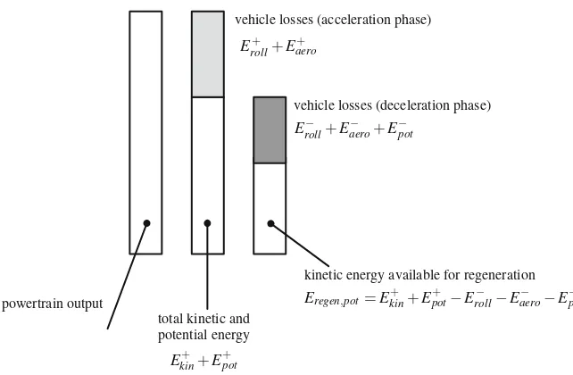
When the vehicle decelerates, it needs to dissipate the entire amount of kinetic energy accumulated during acceleration. The dissipative resistances contribute to this, since they tend to slow down the vehicle. However, the amount of kinetic energy to dissipate during deceleration may be higher than the sum of rolling and aerodynamic resistance; in this case, the vehicle must be decelerated using additional actuators, for example using mechanical brakes or, in a hybrid vehicle, producing negative torque with electric traction motors, thus recuperating (some of) the energy. The amount of energy available for regeneration,Eregen,pot, is the total vehicle energy
cumulated during acceleration (kinetic and potential) minus the losses during the deceleration phase, given by dissipative losses (rolling resistance and aerodynamic drag) and by the increase of potential energy (Epot−)3:
Eregen,pot =Ekin+ +Epot+ −Eroll− −Eaero− −Epot− (2.12)
The diagram in Fig.2.5shows graphically this concept: proceeding from left to right, losses are subtracted to compute the energy available at each stage.
2.3.4
Driving Cycles
As implied in the previous section, the advantages of hybrid vehicles depend on how the vehicle is used. In particular, the hybridization advantages consist essentially in
kinetic energy available for regeneration
total kinetic and potential energy
vehicle losses (acceleration phase)
vehicle losses (deceleration phase)
powertrain output Eregen,pot=E
+
kin+E+pot−Eroll− −Ea−ero−Epot−
Ek+in+Epot+
Eroll+ +Ea+ero
E−
roll+Ea−ero+Epot−
Fig. 2.5 Vehicle energy balance (bar length represents energy)
recovering potential and kinetic energy that would otherwise be dissipated in the brakes, and in operating the engine in its highest-efficiency region. If the engine had a constant efficiency and the vehicle drove at constant speed on a flat road, there would be no advantage in a hybrid electric configuration.
Adriving cyclerepresents both the way the vehicle is driven during a trip and the road characteristics. In the simplest case, it is defined as a time history of vehicle speed (and therefore acceleration) and road grade. Together with the vehicle characteristics, this completely defines the road load, i.e., the force that the vehicle needs to exchange with the road during the driving cycle.
As pointed out in Sect.2.3.3, each term in the energy balance is a function of both the driving cycle (speed, acceleration, grade) and the vehicle (mass, frontal area, coefficients of aerodynamic and rolling resistance). For this reason, the fuel consumption of a vehicle must always be specified in reference to a specific driving cycle. On the other hand, given a driving cycle, the absolute value of the road load and also therelativemagnitude of its components depend on the vehicle characteristics. The necessity for a standard method to evaluate emissions and fuel consumption of all vehicles on the market, and to provide a reliable basis for their comparison, led to the introduction of a reduced number of regulatory driving cycles: any vehicle sold must be tested, according to detailed procedures, using one or more of these standard cycles, which are different for each world region.
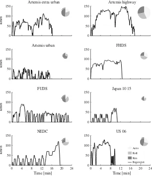
Examples of standard cycles are shown in Fig.2.6, which also include a basic energy analysis comparison.
2.3 Vehicle-Level Energy Analysis 17
0 50 100 150
Artemis extra urban
km/h
Fig. 2.6 Some examples of standard driving cycles. The pie chart shows the relative amount of the energy termsEkin+,E+
aero,Eroll+ , as well as the amount of kinetic energy that can be recovered
according to (2.12). The pie surface is proportional to the total cycle energyEpwt+ defined by (2.11). Energies are computed with the vehicle data of Table8.1
while the others reproduce measures of vehicle speed in actual roads. However, with the exception of US 06, the acceleration levels are well below the capabilities of any modern car, therefore the fuel consumption results are typically optimistic and unable to reproduce real-world driving conditions.
driver his or her own driving style. In order to obtain more realistic estimations of real-world fuel consumption for a specific vehicle, vehicle manufacturers may develop their own testing cycles.
2.4
Powertrain Components
This section contains a description of models of the principal powertrain components suitable for energy flow modeling, neglecting component dynamics. Detailed behav-ioral models accurately accounting for dynamic effect are beyond the objectives of this book and can be found in specialized works.
2.4.1
Internal Combustion Engine
The following modeling approaches can be used for an internal combustion engine, in order of increasing complexity:
1. Static map;
2. Static map and lumped-parameter dynamic model; 3. Mean-value model;
4. One-dimensional fluid-dynamic model;
5. Three-dimensional fluid-dynamic model (finite-element).
The latter two approaches are necessary only for detailed studies focused on the engine subsystem, while the first three methods can be useful in models in which the engine is seen as part of a more comprehensive system (powertrain or vehicle) and as such can be employed in energy management simulators (map models) or powertrain control strategies (map with lumped-parameter dynamics or mean-value models).
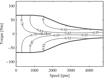
The static map approach assumes the engine to be a perfect actuator, which responds immediately to the commands; the fuel consumption is computed using a map (table) as a function of the engine speed and torque, both of which are assumed to be known. In particular, the torque is typically a control input for the engine, while the speed is a measured input and derives from the coupling to the rest of the pow-ertrain. A curve that gives the maximum engine torque as a function of the current speed is also present in this kind of models to ensure that the torque does not exceed the limits of the engine. Figure2.7shows the typical engine map information with fuel consumption or iso-efficiency contours, the maximum torque curve, and the optimal operation line (OOL), i.e., the combination of torque and speed that provide the maximum efficiency for any given power output. The OOL information is often used in designing heuristic energy management strategies, as a target for the engine operating points.
2.4 Powertrain Components 19
1000 2000 3000 4000 5000 0
1000 2000 3000 4000 5000
0.35
Fig. 2.7 Example of engine fuel consumption map and efficiency map (with optimal operation line, OOL, indashed-line)
by coupling it to a transfer function representing air/fuel dynamics and, possibly, to an inertia representing the crankshaft dynamics.
2.4.2
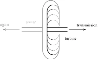
Torque Converter
The torque converter is a fluid coupling device that is used to transmit motion from the engine to the transmission input shaft. It is capable of multiplying the engine torque (acting as a reduction gear), and, unlike most other mechanical joints, provides extremely high damping capabilities, since all torque is transmitted through fluid-dynamic forces rather than friction or pressure. It is traditionally used in vehicles with automatic transmissions as a launching device, because it allows for large speed differences between its two shafts while multiplying the input torque.
A torque converter (Fig.2.8) is composed by three co-axial elements: a pump (also called impeller), connected to the engine shaft, a turbine, connected to the transmission, and a stator in between. The fluid in the torque converter is moved by
the pump because of engine rotation, drags the turbine, and therefore transmits torque to the transmission. The torque at the turbine is multiplied with respect to the pump torque (i.e., the engine torque), thanks to the presence of the stator which modifies the flow characteristics inside the converter. The torque multiplication increases with the speed difference between the pump and the turbine; at steady state, the two elements rotate at the same speed and the torque multiplication factor is unitary.
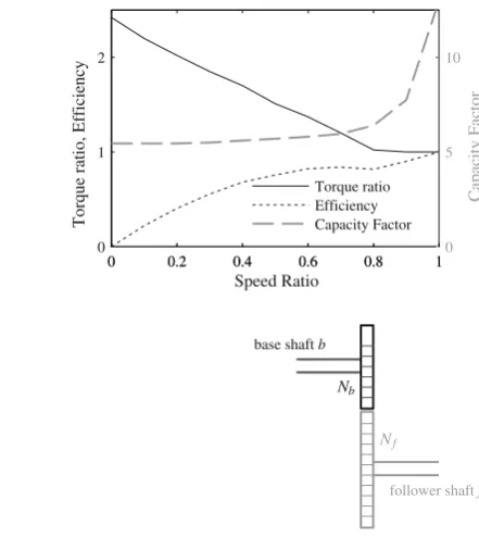
The torque converter model is based on tabulated characteristics of torque ratio and capacity factor versus speed ratio. The speed ratio is
SR= ωt
ωp
, (2.13)
whereωtis the turbine speed andωp the pump speed. The torque ratio or
multipli-cation ratio is
MR= Tt Tp
, (2.14)
withTtandTpthe turbine and pump torque respectively. The capacity factor, which
is a measure of how much torque the torque converter can transmit, is defined as
Ktc= ωp
Tp
. (2.15)
As an alternative to the capacity factor, the torque at 2000 rpm (MP2000) is
some-times used to characterize the torque capacity; it is related to the capacity factor as follows:
MP2000=
20002 K2
tc
, (2.16)
whereKtcmust be expressed in units of√RPMNm.
Examples of characteristic curves of a torque converter are shown in Fig.2.9. The map can be replaced by an analytical model, the Kotwicki model [6], based on curve fitting.
2.4.3
Gear Ratios and Mechanical Gearbox
Gearings are purely mechanical components, with no control, that change the speed and torque transmitted between two shafts without altering the power flow. In prac-tice, however, losses due to friction occur and reduce the output power with respect to the input power.
The simplest model for a gearing only accounts for the speed and torque ratios, without considering the losses due to friction. Indicating with the subscriptsbandf the base and follower shaft (see Fig.2.10), and withgfb= NNb
2.4 Powertrain Components 21
(Nis the number of teeth of each gear), the lossless gear model is:
ωf =gfbωb,
Tf =g1fbTb.
(2.17)
For energy analysis and in general for more accurate predictions, a lossy gear model is introduced, which takes into account power losses. Given that the speed ratio is fixed, being given by kinematic constraints, the speed equation remains the same as the lossless model, while the power loss means a reduction of the torque at the output shaft, described using the gear efficiencyηfb:
Tf =
with the convention that power flow is positive when going frombtof, i.e., whenb is the input shaft. The power loss is always positive and is calculated as
Ploss=
ωbTb(1−ηfb) ifPb =Tb·ωb ≥0,
ωfTf(1−ηfb) ifPb =Tb·ωb <0.
Functionally, a gearbox is a gearing whose transmission ratio (and possibly other characteristics, such as efficiency) can change dynamically. The simplest model for a gearbox consists in a lossy gear with variable gear ratio; the efficiency can be assumed constant or variable with gear ratio, speed, and input torque. This model captures the essential functionality common to manual gearboxes and automatic transmissions, and can be used for both cases. A complete transmission model with several degrees of freedom (considering all the gears, coupling and actuators) is more suited for drivability studies.
2.4.4
Planetary Gear Sets
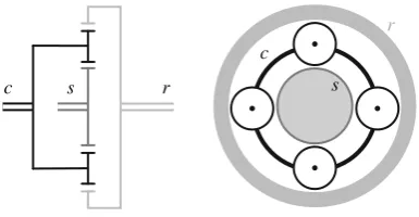
Planetary gear sets are composed by three rotating elements (sun, carrier, and ring) which are connected by internal gears (planets); stopping one of the three shafts gen-erates a fixed gear ratio between the remaining two. Planetary gears are commonly used in traditional automatic transmissions because they allow for compact construc-tion and smooth gear transiconstruc-tion. They are often present in hybrid electric vehicles to realize electrically variable transmissions (EVTs) by connecting the engine and two electric machines to the three shafts of the gear set.
A schematic representation of a planetary gear set is shown in Fig.2.11. The tangential speed of the carrier (at the center of the planets, i.e., at a radius intermediate between sun and ring) is the average of the sun and ring speeds. Indi-cating with the subscriptss,r, andcthe sun, ring, and carrier shafts, the following kinematic constraint can be written:
ωc(Nr+Ns)=(ωrNr+ωsNs) , (2.20)
whereNrandNsare the number of teeth of the ring and sun gear, respectively. The
reason for writing this relation in terms of number of teeth instead of radii is that—in a given gear set—the number of teethNof each gear is directly proportional to the radius of the respective gear.
Introducing the planetary gear ratioρ=Ns/Nr(the ratio of the number of teeth
of sun to the number of teeth of the ring), the kinematic relation (2.20) is written in
Fig. 2.11 Schematic representation of planetary gear set
c s r
r
c
2.4 Powertrain Components 23
Fig. 2.12 Torque balance on the planets
Tc
(Ns+Nr)/2 Ts
Ns
Tr
Nr
the more compact form:
(1+ρ)ωc=ρωs+ωr. (2.21)
The torque at the carrier at steady state is equally split between the sun and the ring; for the equilibrium of the planets (Fig.2.12), the following torque equations hold:
Tc
(Nr+Ns) =
Tr
Nr
, (2.22a)
Tc
(Nr+Ns)=
Ts
Ns
, (2.22b)
where, again, the number of teeth are used instead of the radii. Using the planetary gear ratioρ=Ns/Nr, the equilibrium equations become:
Tc=(1+ρ)Tr, (2.23a)
Ts=ρTr. (2.23b)
Equations (2.21) and (2.23a,2.23b) are the basis for modeling planetary gear sets. The torque equations (2.23a,2.23b) are only valid in steady-state conditions and neglect losses, but can be used with reasonable accuracy in vehicle-level models.
2.4.5
Wheels, Brakes, and Tires
The wheel represents the link between the powertrain and the external environment. Its model includes the motion of the wheel and the effect of the brakes, calculating the forces at the interface between tire and road surface. The tractive force is calculated given the powertrain torque, the brake signal and the vertical load on the wheel. A quasi-static model is usually sufficient, while dynamic tire models (see, for example, [4]) are typically used in models for vehicle lateral dynamics (handling models).
pure rolling motion between the tire and the road, and neglecting tire deformation. These hypotheses work well for driving in normal conditions (not extreme accelera-tions) on roads with good adherence (dry asphalt). Low-adherence roads or extreme maneuvers require more accurate tire models to predict vehicle behavior in terms of speed dynamics.
The brakes can be modeled as an additional torque that reduces the net torque acting on the tire. The brake torque is proportional to the brake input signal. Therefore the net tractive force acting on the wheels is
Ftrac=
where Tpwt is the torque generated by the powertrain at the wheel shaft,Tbrakethe
braking torque, andRwhthe wheel radius.
The wheel speed is
ωwh=
vveh
Rwh
, (2.25)
beingvvehthe longitudinal vehicle speed.
The value of longitudinal force is bounded by the vertical load acting on the wheel:
−Fzνx,max ≤Ftrac≤Fzνx,max, (2.26)
whereFzis the vertical force on the wheel, andνx,maxis the peak value of the road/tire
friction coefficient (usually around 0.8–0.9 for dry asphalt). In order to maintain proper vehicle stability and maximize braking efficiency, the braking action must be distributed between front and rear axles according to the normal load acting on each, also accounting for the longitudinal load transfer generated by the deceleration. From (2.1), the total tractive force during braking is:
Ftrac=Mvehv˙veh+Froll+Faero+Fgrade. (2.27)
This should be distributed between the front and rear axle (f andr) proportionally to the vertical load on each, i.e.:
Ftrac,f
where a andbare the distances of the center of gravity (CG) from the front and rear axle respectively, andhCGits height from the ground. The terms that include
the accelerationv˙vehrepresent the dynamic load transfer, from the rear axle to the
2.4 Powertrain Components 25
acceleration. In most passenger vehicles, the powertrain generates torque only on one of the two axles. In that case, regenerative braking can only be applied to that axle, and must be appropriately balanced by conventional braking on the other axle. From the energy management standpoint, this means that not all the braking torque can be regenerated, but only the fraction of it that is applied at the traction axle, i.e., (2.28) for front-wheel drive or (2.29) for rear-wheel drive vehicles.
2.4.6
Electric Machines
The electric machines can be modeled using an approach similar to the one used for the engine, i.e., based on maps of torque and efficiency. Desired values of electrical power or torque can be used as a control input. Rotor inertia is the main dynamic element that is usually modeled, as the electrical dynamics are very fast in comparison with the inertial dynamics or the engine dynamics.
The relation between torque at the shaft and electric power is provided by an efficiency map, which can be expressed as a function of speed and torque, or speed and electrical power (depending on the implementation).
The efficiency map can also include the power electronics between the main electric bus and the machine to provide directly the electric power exchanged with the battery; otherwise, an explicit power electronics efficiency should be included in the model between the electric machine and the battery.
The efficiency model can be expressed as,
Pmech=ωem·Tem =
ηem(ωem,Pelec)·Pelec ifPelec≥0 (motoring mode),
1
ηem(ωem,Pelec)Pelec ifPelec<0 (generating mode),
(2.30) or, if electric power is the desired output, as
Pelec=
1
η(ωem,Tem)Pmech=
1
ηem(ωem,Tem)ω·Tem ifPelec≥0 (motoring mode),
ηem(ωem,T)·Pmech=ηem(ωem,Tem)·ωem·Tem ifPelec<0 (generating mode).
(2.31)
An example of efficiency map for an electric motor is shown in Fig.2.13.
2.4.7
Batteries
Fig. 2.13 Example of electric motor efficiency map (elaboration of data in [7])
0.75
0 1000 2000 3000 4000
−100 −50 0 50 100
Accurately modeling battery dynamics in hybrid electric vehicles is critical and not trivial, because the main variables that characterize battery operation, i.e. state of charge, voltage, current and temperature, are dynamically related to each other in a highly nonlinear fashion. In general, the objective of the battery model in a vehicle simulator is to predict the change in state of charge given the electrical load.
The state of charge (SOC) is defined as the amount of electrical charge stored in the battery, relative to the total charge capacity:
SOC(t)= Q(t)
Qnom
, (2.32)
whereQnomis the nominal charge capacity, andQ(t)the amount of charge currently
stored. TheSOCdynamics are given by:
˙
where I is the battery current (positive during discharge),ηcoul is the Coulombic
efficiency [1] or charge efficiency, which accounts for charge losses and depends on current operating conditions (mainly current intensity and temperature).
Calculating the state of charge (or, better, its variation) by integration of (2.33) appears to be relatively straightforward, if the capacity is assumed to be a constant, known parameter. In reality, the battery capacity and coulombic efficiency change according to several parameters, and the numerical integration is reliable only in simulation in the absence of measurement error and noise, which makes reliable state of charge estimation a significant portion of the actual battery management system (BMS) [8].
In order to correlate the battery current and voltage to the power exchanged with the rest of the powertrain, a circuit model of the battery can be used.
2.4 Powertrain Components 27
+
Voc I
VL
R1
R0
C1 C2
R2
V1 V2
Fig. 2.14 Battery equivalent circuit-based model (second-order)
Fig. 2.15 Battery circuit model (no dynamics)
Voc
VL
I
+ R0
The series resistanceR0represents the Ohmic losses due to actual resistance of
the wires and the electrodes and also to the dissipative phenomena that reduce the net power available at the terminals; the resistancesR1,R2and the capacitancesC1,C2
are used to model the dynamic response of the battery. The values of the parameters are estimated using curve fitting of experimental data, and are generally variable with the operating conditions (temperature, state of charge, current directionality). Other models of the same kind, with more or fewer R–C branches in series, can be used depending on the required model accuracy. However, the number of parameters to be identified increases with the model order. Very often, simpler models without any R–C branch (Fig.2.15) can also be used if the voltage dynamics can be neglected, for example in quasi-static models focusing exclusively on efficiency considerations. When no detailed data from battery testing is available, circuit models with a single, constantR0may be the only option.
The equations of the circuit in Fig.2.14are:
VL=Voc−R0I−
n
i=1
Vi, (2.34)
Ci
dVi
dt =I− Vi
Ri
, (2.35)
whereVLis the load voltage at the battery terminals,Vocis the open circuit voltage,
i.e., the voltage of the battery when it is not connected to any load (I =0),R0the series
Riand the capacitanceCi),nis the order of the dynamic model considered, i.e., the
number of R–C branches. In the example shown,n=2. The capacitanceCiand the
resistanceRican change with the direction (charge or discharge) and amplitude of
the current and with other operating conditions, such as temperature and state of charge; the variation can be taken into account by expressing the parameters as maps (tables) instead of constants.
If voltage dynamics are neglected and the battery circuit is represented without R–C branches as in Fig.2.15, the circuit equation is easily written as a function of the terminal powerPbatt:
Pbatt =VL·I =VocI−R0I2, (2.36)
thus providing an explicit expression of the current as a function of power:
I= Voc
The circuit representation of Figs.2.14and2.15and the corresponding equations are referred to the entire battery pack. This is usually composed by many cells connected in series (strings), and possibly several strings in parallels. The electrical parameters of the circuit models are those of the entire pack, which can be computed from the values of each cell as follows:
Voc=NSVoc,cell, (2.38)
where NS is the number of cells in series in each string, andNP is the number of
strings in parallel.4
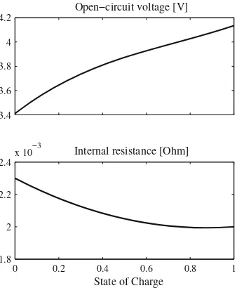
The open circuit voltageVocis a typical characteristic of the battery (or, better, of
its cells) and is primarily a function of the state of charge. An example of variation of the open circuit voltage Voc with the state of charge for a single Li-Ion cell is
shown in Fig.2.16. The figure also shows the internal resistance of the same cell. It is common practice to refer to the value of the current in terms of its C-rate, i.e., as a fraction of the battery capacity (expressed in Ah): for example, if the capacity is 6.5 Ah, a current of 1 C corresponds to 6.5 A, 10 C–65 A, 0.1 C–0.65 A. Steady-state characteristics of the battery, such as those of Fig.2.16, are typically obtained using a current of 1 C.