Introduction to
Operations Research
Deterministic Models
J
URAJ
STACHO
Contents
1 Mathematical modeling by example 1
1.1 Activity-based formulation . . . 3
2 Linear Programming 5 2.1 Formulating a linear program. . . 5
2.2 Summary and further tricks . . . 8
3 Solving linear programs 10 3.1 Graphical method . . . 10
3.2 Fourier-Motzkin Elimination (FME) . . . 13
4 Simplex method 16 4.1 Canonical form . . . 16
4.2 Simplex method by example . . . 17
4.3 Two phase Simplex method. . . 21
4.4 Special cases . . . 21
4.5 Phase I. . . 23
5 Linear Algebra Review 27 5.1 Systems of linear equations . . . 29
5.2 Summary . . . 31
6 Sensitivity Analysis 33 6.1 Changing the objective function . . . 35
6.2 Changing the right-hand side value . . . 37
6.3 Detailed example . . . 39
6.4 Adding a variable/activity. . . 43
iii
6.5 Adding a constraint . . . 43
6.6 Modifying the left-hand side of a constraint . . . 44
7 Duality 45 7.1 Pricing interpretation . . . 45
7.2 Duality Theorems and Feasibility. . . 47
7.3 General LPs . . . 47
7.4 Complementary slackness . . . 48
8 Other Simplex Methods 52 8.1 Dual Simplex Method. . . 52
8.2 Upper-Bounded Simplex . . . 54
8.3 Lower bounds . . . 55
8.4 Dual Simplex with Upper Bounds . . . 56
8.5 Goal Programming . . . 57
9 Transportation Problem 59 9.1 Transportation Simplex Method . . . 60
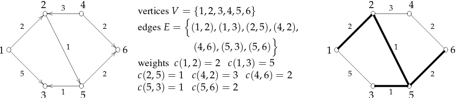
10 Network problems 65 10.1 Shortest Path Problem. . . 66
10.2 Minimum Spanning Tree . . . 68
10.3 Maximum Flow problem . . . 69
10.4 Minimum-cost Flow problem. . . 72
10.5 Network Simplex Algorithm . . . 72
10.6 Network Simplex Algorithm with capacitites . . . 76
10.7 Complete example . . . 77
10.8 Summary . . . 83
11 Game Theory 85 11.1 Pure and Mixed strategies. . . 86
11.2 Nonconstant-sum Games . . . 88
12 Integer programming 89 12.1 Problem Formulation . . . 89
12.2 Cutting Planes. . . 92
12.3 Branch and Bound . . . 95
Preface
These lecture notes were written during the Fall/Spring 2013/14 semesters to accompany lectures of the course
IEOR 4004: Introduction to Operations Research - Deterministic Models. The notes were meant to provide a succint summary of the material, most of which was loosely based on the bookWinston-Venkataramanan: Introduction to Mathematical Programming (4th ed.), Brooks/Cole 2003. Other material (such as the dictionary notation) was adapted fromChv´atal: Linear Programming, Freeman 1983andDantzig-Thapa: Linear Programming, Springer-Verlag 1997. Various other bits were inspired by other lecture notes and sources on the Internet. These notes are not meant to replace any book; interested reader will find more details and examples in the Winston book in particular. I would like to thank students that helped me correct numerous mistakes in the earlier versions of the notes. Most likely all mistakes have not been yet caught, and so the reader should exercise caution should there be inconsistencies in the text. I am passing on the notes to Prof. Strickland who will continue making adjustments to the material as needed for the upcoming offerings of the course. Of course, any suggestions for improvements are welcomed from anyone interested.
Juraj Stacho July 26, 2014
1
Mathematical modeling by example
Product mix
A toy company makes two types of toys: toy soldiers and trains. Each toy is produced in two stages, first it is constructed in a carpentry shop, and then it is sent to a finishing shop, where it is varnished, vaxed, and polished. To make one toy soldier costs $10 for raw materials and $14 for labor; it takes 1 hour in the carpentry shop, and 2 hours for finishing. To make one train costs $9 for raw materials and $10 for labor; it takes 1 hour in the carpentry shop, and 1 hour for finishing.
There are 80 hours available each week in the carpentry shop, and 100 hours for finishing. Each toy soldier is sold for $27 while each train for $21. Due to decreased demand for toy soldiers, the company plans to make and sell at most 40 toy soldiers; the number of trains is not restriced in any way.
What is the optimum (best) product mix (i.e., what quantities of which products to make) thatmaximizesthe profit (assuming all toys produced will be sold)?
Terminology
decision variables: x1,x2, . . . ,xi, . . .
variable domains: values that variables can take x1,x2≥0
goal/objective: maximize/minimize
objective function: function to minimize/maximize 2x1+5x2
constraints: equations/inequalities 3x1+2x2≤10
Example
Decision variables: • x1= # of toy soldiers • x2= # of toy trains Objective: maximize profit
• $27−$10−$14=$3profit for selling one toy soldier⇒3x1profit (in $) for sellingx1toy soldier • $21−$9−$10=$2profit for selling one toy train⇒2x2profit (in $) for sellingx2toy train ⇒ z=3x1+2x2
| {z }
objective function
profit for sellingx1toy soldiers andx2toy trains
2 CHAPTER 1. MATHEMATICAL MODELING BY EXAMPLE
Constraints:
• producingx1toy soldiers andx2toy trains requires
(a) 1x1+1x2hours in the carpentry shop; there are 80 hours available
(b) 2x1+1x2hours in the finishing shop; there are 100 hours available • the numberx1of toy soldiers produced should be at most 40
Variable domains: the numbersx1,x2of toy soldiers and trains must be non-negative (sign restriction) Max 3x1 + 2x2
x1 + x2 ≤ 80
2x1 + x2 ≤ 100
x1 ≤ 40 x1,x2 ≥ 0
We call this aprogram. It is alinearprogram, because the objective is a linear function of the decision variables, and the constraints are linear inequalities (in the decision variables).
Blending
A company wants to produce a certain alloy containing 30% lead, 30% zinc, and 40% tin. This is to be done by mixing certain amounts of existing alloys that can be purchased at certain prices. The company wishes to minimize the cost. There are 9 available alloys with the following composition and prices.
Alloy 1 2 3 4 5 6 7 8 9 Blend
Lead (%) 20 50 30 30 30 60 40 10 10 30
Zinc (%) 30 40 20 40 30 30 50 30 10 30
Tin (%) 50 10 50 30 40 10 10 60 80 40
Cost ($/lb) 7.3 6.9 7.3 7.5 7.6 6.0 5.8 4.3 4.1 minimize
Designate adecisionvariablesx1,x2, . . . ,x9where
xiis theamountof Alloyiin aunit of blend
In particular, the decision variables must satisfyx1+x2+. . .+x9 = 1. (It is a common mistake to choosexi the
absoluteamount of Alloyiin the blend. That may lead to a non-linear program.) With that we can setup constraints and the objective function.
Min 7.3x1 + 6.9x2 + 7.3x3 + 7.5x4 + 7.6x5 + 6.0x6 + 5.8x7 + 4.3x8 + 4.1x9 = z [Cost]
s.t. x1 + x2 + x3 + x4 + x5 + x6 + x7 + x8 + x9 = 1
0.2x1 + 0.5x2 + 0.3x3 + 0.3x4 + 0.3x5 + 0.6x6 + 0.4x7 + 0.1x8 + 0.1x9 = 0.3 [Lead] 0.3x1 + 0.4x2 + 0.2x3 + 0.4x4 + 0.3x5 + 0.3x6 + 0.5x7 + 0.3x8 + 0.1x9 = 0.3 [Zinc] 0.5x1 + 0.1x2 + 0.5x3 + 0.3x4 + 0.4x5 + 0.1x6 + 0.1x7 + 0.6x8 + 0.8x9 = 0.4 [Tin] Do we needallthe four equations?
Product mix (once again)
1.1. ACTIVITY-BASED FORMULATION 3
Chair 1 Chair 2 Chair 3 Chair 4 Total available
Steel 1 1 3 9 4,4000 (lbs)
Wood 4 9 7 2 6,000 (lbs)
Profit $12 $20 $18 $40 maximize
Decision variables:
xi=the number of chairs of typeiproduced
eachxiis non-negative
Objective function:
maximize profitz=12x1+20x2+18x3+40x4
Costraints:
at most4, 400lbs of steel available:x1+x2+3x3+9x4≤4, 400
at most6, 000lbs of wood available:4x1+9x2+7x3+2x4≤6, 000
Resulting program:
Max 12x1 + 20x2 + 18x3 + 40x4 = z [Profit]
s.t. x1 + x2 + 3x3 + 9x4 ≤ 4, 400 [Steel]
4x1 + 9x2 + 7x3 + 2x4 ≤ 6, 000 [Wood]
x1,x2,x3,x4≥0
1.1
Activity-based formulation
Instead of constructing the formulation as before (row-by-row), we can proceed by columns. We can view columns of the program asactivities. An activity has
inputs: materials consumed per unit of activity (1lb of steel and 4lbs of wood) outputs: products produced per unit of activity ($12 of profit) activity level: a level at which we operate the activity (indicated by a variablex1)
Chair 1
x1
1lb of steel
4lbs of wood $12 of profit
inputs activity outputs
Operating the activity “Chair 1” at levelx1means that we producex1chairs of type 1, each consuming 1lb of steel, 4lbs of wood, and producing $12 of profit. Activity levels are always assumed to benon-negative.
The materials/labor/profit consumed or produced by an activity are calleditems(correspond to rows).
The effect of an activity on items (i.e. the amounts of items that are consumed/produced by an activity) areinput-output coefficients.
The total amount of items available/supplied/required is called theexternal flow of items. We chooseobjectiveto be one of the items which we choose to maximize or minimize.
4 CHAPTER 1. MATHEMATICAL MODELING BY EXAMPLE
Example
Items: Steel Wood Profit
External flow of items:
Steel: 4,400lbs of available (flowing in) Wood: 6,000lbs of available (flowing in) Objective:
Profit: maximize (flowing out) Activities:
producing a chair of typeiwherei=1, 2, 3, 4, each is assigned an activity levelxi
Chair 1: Producing 1 chair of type 1 consumes 1 lb of Steel
4 lbs of Wood produces $12 of Profit
Chair 1
x1
1lb of Steel
4lbs of Wood $12 of Profit
Chair 2: Producing 1 chair of type 2 consumes 1 lb of Steel
9 lbs of Wood produces $20 of Profit
Chair 2
x2
1lb of Steel
9lbs of Wood $20 of Profit
Chair 3: Producing 1 chair of type 3 consumes 3 lbs of Steel
7 lbs of Wood produces $18 of Profit
Chair 3
x3
3lbs of Steel
7lbs of Wood $18 of Profit
Chair 4: Producing 1 chair of type 4 consumes 9 lbs of Steel
2 lbs of Wood produces $40 of Profit
Chair 4
x4
9lbs of Steel
2lbs of Wood $40 of Profit
The material balance equations:
To see how to do this, consider activity Chair 1: consumes 1lb of Steel, 4lbs of Wood, and produces $12 of Profit. Thus at levelx1, we consume1x1lbs of Steel,4x1lbs of Wood, and produce12x1dollars of Profit.
Chair 1
x1
1lb of Steel
4lbs of Wood $12 of Profit
. . .+ 12x1 + . . . [Profit]
. . .+ 1x1 + . . . [Steel]
. . .+ 4x1 + . . . [Wood]
On the right, you see the effect of operating the activity at levelx1. (Note in general we will adopt a differentsign convention; we shall discuss is in a later example.)
Thus considering all activities we obtain:
12x1 + 20x2 + 18x3 + 40x4 [Profit]
x1 + x2 + 3x3 + 9x4 [Steel]
4x1 + 9x2 + 7x3 + 2x4 [Wood]
Finally, we incorporate the external flow and objective: 4,400lbs of Steel available, 6, 000lbs of Wood available, maximize profit:
Max 12x1 + 20x2 + 18x3 + 40x4 = z [Profit]
s.t. x1 + x2 + 3x3 + 9x4 ≤ 4, 400 [Steel]
4x1 + 9x2 + 7x3 + 2x4 ≤ 6, 000 [Wood]
2
Linear Programming
Linear program (LP) in astandard form(maximization)
max c1x1 + c2x2 + . . . + cnxn Objective function
subject to a11x1 + a12x2 + . . . + a1nxn ≤ b1 a21x1 + a22x2 + . . . + a2nxn ≤ b2
..
. + ... ... ...
am1x1 + am2x2 + . . . + amnxn ≤ bm
x1,x2, . . . ,xn ≥ 0 Sign restrictions
Constraints
Feasible solution(point) P = (p1,p2, . . . ,pn)is an assignment of values to the p1, . . . ,pnto variablesx1, . . . ,xn
that satisfiesallconstraints andallsign restrictions. Feasible region≡the set of all feasible points.
Optimal solution≡a feasible solution with maximum value of the objective function.
2.1
Formulating a linear program
1. Choose decision variables
2. Choose an objective and an objective function – linear function in variables 3. Choose constraints – linear inequalities
4. Choose sign restrictions
Example
You have $100. You can make the following three types of investments:
Investment A.Every dollar invested now yields $0.10 a year from now, and $1.30 three years from now. Investment B.Every dollar invested now yields $0.20 a year from now and $1.10 two years from now. Investment C.Every dollar invested a year from now yields $1.50 three years from now.
During each year leftover cash can be placed into money markets which yield 6% a year. The most that can be invested a single investment (A, B, or C) is $50.
Formulate an LP to maximize the available cash three years from now.
6 CHAPTER 2. LINEAR PROGRAMMING
Decision variables:xA,xB,xC, amounts invested into Investments A, B, C, respectively
y0,y1,y2,y3cash available/invested into money markets now, and in 1,2,3 years.
Max y3
s.t. xA + xB + y0 = 100
0.1xA + 0.2xB − xC + 1.06y0 = y1
1.1xB + 1.06y1 = y2
1.3xA + 1.5xC + 1.06y2 = y3
xA ≤ 50
xB ≤ 50
xC ≤ 50
xA,xB,xC,y0,y1,y2,y3 ≥ 0
Items
Activities
z }| {
Inv. A Inv. B Inv. C Markets Now
Markets Year 1
Markets Year 2
External flow
Now −1 −1 −1 = −100
Year1 0.1 0.2 −1 1.06 −1 = 0
Year2 1.1 1.06 −1 = 0
Year3 1.3 1.5 1.06 maximize
Sign convention:inputs havenegativesign, outputs havepositivesigns. External in-flow hasnegativesign, external out-flow haspositivesign.
We have in-flow of$100cash “Now” which means we have−$100on the right-hand side. No in-flow or out-flow of any other item.
Inv. A
xA
$1 Now
$0.1 Year1 $1.3 Year3
Markets Now
y0
$1 Now $1.06 Year1
Inv. B
xB
$1 Now
$0.2 Year1 $1.1 Year2
Markets Year 1
y1
$1 Year1 $1.06 Year2
Inv. C
xC
$1 Year1 $1.5 Year3
Markets Year 2
y2
$1 Year2 $1.06 Year3
Max 1.3xA + 1.5xC + 1.06y2
s.t. xA + xB + y0 = 100
0.1xA + 0.2xB − xC + 1.06y0 − y1 = 0
1.1xB + 1.06y1 − y2 = 0
y0, y1, y2 ≥0
2.1. FORMULATING A LINEAR PROGRAM 7
Post office problem
Post office requires different numbers of full-time employees on different days. Each full time employee works 5 consecutive days (e.g. an employee may work from Monday to Friday or, say from Wednesday to Sunday). Post office wants to hire minimum number of employees that meet its daily requirements, which are as follows.
Monday Tuesday Wednesday Thursday Friday Saturday Sunday
17 13 15 19 14 16 11
Letxidenote the number of employees thatstart workingin dayiwherei=1, ..., 7and work for 5 consecutive days
from that day. How many workers work on Monday? Those that start on Monday, or Thursday, Friday, Saturday, or Sunday. Thusx1+x4+x5+x6+x7should be at least17.
Then the formulation is thus as follows:
min x1 + x2 + x3 + x4 + x5 + x6 + x7
s.t. x1 + x4 + x5 + x6 + x7 ≥ 17
x1 + x2 + x5 + x6 + x7 ≥ 13
x1 + x2 + x3 + x6 + x7 ≥ 15
x1 + x2 + x3 + x4 + x7 ≥ 19 x1 + x2 + x3 + x4 + x5 ≥ 14 x2 + x3 + x4 + x5 + x6 ≥ 16 x3 + x4 + x5 + x6 + x7 ≥ 11 x1, x2, . . . , x7 ≥ 0
Monday Tuesday Wednesday Thursday Friday Saturday Sunday
Total 1 1 1 1 1 1 1 minimize
Monday 1 1 1 1 1 ≥ 17
Tuesday 1 1 1 1 1 ≥ 13
Wednesday 1 1 1 1 1 ≥ 15
Thursday 1 1 1 1 1 ≥ 19
Friday 1 1 1 1 1 ≥ 14
Saturday 1 1 1 1 1 ≥ 16
Sunday 1 1 1 1 1 ≥ 11
(Simple) Linear regression
Given a set of datapoints{(1, 2),(3, 4),(4, 7)}we want to find a line that most closely represents the datapoints. There are various ways to measure what it means ”closely represent”. We may, for instance, minimize the average distance (deviation) of the datapoints from the line, or minimize the sum of distances, or the sum of squares of distances, or minimize the maximum distance of a datapoint from the line. Here the distance can be either Euclidean distance, or vertical distance, or Manhattan distance (vertical+horizontal), or other.
We choose to minimize the maximum vertical distance of a point from the line. A general equation of a line with finite slope has formy=ax+cwhereaandcare parameters. For a point(p,q), the vertical distance of the point from the liney=ax+ccan be written as|q−ap−c|. Thus we want
Problem: Find constantsa,csuch that the largest of the three values|2−a−c|,|4−3a−c|,|7−4a−c|is as small as possible.
min maxn2−a−c, 4−3a−c, 7−4a−c
o
We want to formulate it as a linear program. Issues: non-negativity, the absolute value, the min of max.
8 CHAPTER 2. LINEAR PROGRAMMING
Min w
s.t. w ≥ |2−1a−c| w ≥ |4−3a−c| w ≥ |7−4a−c|
• absolute values:w≥ |i|if and only ifw≥iandw≥ −i.
(in other words, the absolute value ofiis at mostwif and only if−w≤i≤w)
Min w
s.t. w ≥ 2−a−c w ≥ −2+a+c w ≥ 4−3a−c w ≥ −4+3a+c w ≥ 7−4a−c w ≥ −7+4a+c
• unrestricted sign: writex=x+−x−wherex+,x− ≥0are new variables
Min w
s.t. w ≥ 2−a++a−−c++c− w ≥ −2+a+−a−+c+−c− w ≥ 4−3a++3a−−c++c− w ≥ −4+3a+−3a−+c+−c− w ≥ 7−4a++4a−−c++c− w ≥ −7+4a+−4a−+c+−c−
wherea+,a−,c+,c−,w≥0
Min w
s.t. w + a+ − a− + c+ − c− ≥ 2
w − a+ + a− − c+ + c− ≥ −2
w + 3a+ − 3a− + c+ − c− ≥ 4
w − 3a+ + 3a− − c+ + c− ≥ −4
w + 4a+ − 4a− + c+ − c− ≥ 7
w − 4a+ + 4a− − c+ + c− ≥ −7
a+,a−,c+,c−,w ≥ 0
Note
The above formulation on the right isstandardform of a minimization LP. We have already seen the standard form of a maximization problem; this is the same except that we minimize the objective function and the signs of inequalities switch (this is only done for convenience sake when we get to solving LPs).
2.2
Summary and further tricks
Let us summarize what we have learned so far.
• Linear Program (LP) is an optimization problem where
→ thegoalis to maximize or minimize alinear objective function
→ over a set offeasible solutions– i.e. solution of a set oflinear inequalities (forming thefeasible region).
• Standard form: all inequalities are≤-inequalities (or all are≥-inequalities) and all variables are non-negative
→ to get a≤-inequality from a≥-inequality we multiply both sides by−1and reverse the sign (this gives us an equivalent problem)
x1−x2≤100 ⇐⇒ −x1+x2≥ −100
→ to get inequalities from an equation, we replace it by two identical inequalities, one with≤and one with≥
x1−x2=100 ⇐⇒ x1−x2≤100
2.2. SUMMARY AND FURTHER TRICKS 9
→ eachunrestrictedvariable (urs) is replaced by thedifferenceof two new non-negative variables
. . .+x1+. . .
x1urs ⇐⇒
. . . + (x2−x3) + . . .
x2,x3≥0
→ anon-positivevariablex1≤0is replaced by thenegativeof a new non-negative variablex2
. . .+x1+. . .
x1≤0 ⇐⇒
. . . + (−x2) + . . . x2≥0
→ absolutevalue: we can replaceonlyin certain situations
∗ inequalities of type|f| ≤gwheref andgare arbitrary expressions: replace by two inequalities f ≤gand−g≤ f
∗ if+|f|appears in theobjective functionand we areminimizingthis function:
replace+|f|in the objective function by a new variablex1and add a constraint|f| ≤x1. (likewise if−|f|appears when maximizing)
→ min of max: ifmax{f1,f2, . . . ,ft}in theobjective functionand we areminimizing, then replace this
expression with a new variablex1and add constraintsfi≤x1for eachi=1, . . . ,t:
. . . + max{f1, . . . ,ft}+ . . . ⇐⇒ . . . + x1 +. . .
x1urs
f1≤x1 f2≤x1
.. .
ft≤x1
→ unrestricted expressionf can be written as a difference of two non-negative variables
. . .+ f +. . . ⇐⇒ . . . + (x2−x3) + . . .
x2,x3≥0
Moreover, if we areminimizing, we can use+x2and+x3(positivemultiples ofx2,x3) in theobjective function(if maximizing, we can use negative multiples).
In anoptimal solutionthe meaning of these new variables will be as follows: ∗ if f ≥0, thenx2= f andx3=0,
∗ if f <0, thenx2=0andx3=−f.
In other words,x2represents thepositive partoff, andx3thenegative partoff(can you see why?). Note
that this only guaranteed to hold for an optimal solution (but that will be enough for us).
3
Solving linear programs
3.1
Graphical method
Max 3x1 + 2x2 x1 + x2 ≤ 80
2x1 + x2 ≤ 100
x1 ≤ 40 x1,x2 ≥ 0
1. Find the feasible region.
• Plot each constraint as an equation≡line in the plane
• Feasible points on one side of the line – plug in (0,0) to find out which
20 40 60 80 100
20 40 60 80 100 x2
x1 20 40 60 80 100
20 40 60 80 100 x2
x1
x1 + x2✁ 80
Start withx1≥0andx2≥0 addx1+x2≤80
3.1. GRAPHICAL METHOD 11
20 40 60 80 100
20 40 60 80 100 x2
x1
x1 + x2 80
2x1 + x2 100
20 40 60 80 100
20 40 60 80 100 x2
x1
x1✂ 40
x1 + x2✂ 80
2x1 + x2✂ 100
feasible region
add2x1+x2≤100 addx1≤40
Acorner(extreme) pointXof the regionR≡every line throughXintersectsRin a segment whose one endpoint isX. Solving a linear program amounts to finding a best corner point by the following theorem.
Theorem 1. If a linear program has anoptimalsolution, then it also has anoptimal solutionthat is acorner point
of the feasible region.
Exercise.Try to find all corner points. Evaluate the objective function3x1+2x2at those points.
20 60
20 40 60 80 100 x2
x1
feasible region
❝✄☎✆✝☎ points
(40,20) (0,80)
(20,60)
(0,0)
(40,0)
20 60
20 40 60 80 100 x2
x1
feasible region
180 = 3*20 + 2*60
160 = 3*40 + 2*20 160 = 3*0 + 2*80
120 =
= 3*40 + 2*0 3*0 + 2*0 = 0
highest value (optimum)
Problem:there may be too many corner points to check. There’s a better way. Iso-valueline≡in all points on this line the objective function has the same value
For our objective3x1+2x2an iso-value line consists of points satisfying3x1+2x2=zwherezis some number. Graphical Method(main steps):
1. Find the feasible region.
12 CHAPTER 3. SOLVING LINEAR PROGRAMS
3. Slide the line in the direction of increasing value until it only touches the region. 4. Read-off an optimal solution.
20 40 60 80
20 40 60 80 100 x2
x1
z = 3x1 + 2x2 = 0
z = 60 z = 120 z = 180 z = 240
20 40 60
20 40 60 80 100 x2
x1
z = 3x1 + 2x2
Optimal solutionis(x1,x2) = (20, 60).
Observe that this point is the intersection of two lines forming the boundary of the feasible region. Recall that lines we use to construct the feasible region come from inequalities (the points on the line satisfy the particular inequality with equality).
Binding constraint≡constraint satisfied with equality
For solution(20, 60), the binding constraints arex1+x2 ≤ 80and2x1+x2 ≤ 100because 20+60 = 80and
2×20+60=100. The constraintx1≤40is not binding becausex1=20<40.
The constraint is binding because changing it (a little) necessarily changes the optimality of the solution. Any change to the binding constraints either makes the solution not optimal or not feasible.
A constraint that is not binding can be changed (a little) without disturbing the optimality of the solution we found. Clearly we can changex1 ≤ 40tox1 ≤ 30and the solution(20, 60)is still optimal. We shall discuss this more in-depth when we learn about Sensitivity Analysis.
Finally, note that the above process always yields one of the following cases.
Theorem 2. Every linear program has either
(i) auniqueoptimal solution, or
(ii) multiple (infinity) optimal solutions, or (iii) isinfeasible(has no feasible solution), or
3.2. FOURIER-MOTZKIN ELIMINATION (FME) 13
3.2
Fourier-Motzkin Elimination (FME)
A simple (but not yet most efficient) process to solve linear programs. Unlike the Graphical method, this process applies to arbitrary linear programs, but more efficient methods exist. The FME method
finds a solution to a system of linear inequalities
(much like Gaussian elimination from Linear algebra which finds a solution to a system oflinear equations) We shall discuss how this is done for≥-inequalities and forminimizationLPs. (Similarly it can be stated for≤ -inequalities and maximization LPs.) You can skip to the example below to get a better idea.
First, we need to adapt the method to solving linear programs. We need to incorporate the objective function as part of the inequalities. Wereplacethe objective function by anewvariablezand look for a solution to the inequalities such thatzis smallest possible (explained how later).
0. Objective functionc1x1+c2x2+. . .+cnxn: add a new constraintz≥c1x1+c2x2+. . .+cnxn
From this point, we assume that all we have is a system of≥-inequalities with all variables on the left-hand side and a constant on the right-hand side. (We change ≤-inequalities to ≥-inequalities by multiplying by−1.) We proceed similarly as in Gaussian elimination. We try to eliminate variables one by one bypivotting a variable in all inequalities(not just one). Unlike Gaussian elimination, we are dealing with inequalities here and so we arenot allowedto multiply by a negative constant when pivotting. This requires a more complex procedure to eliminatex1.
1. Normalizex1: if+cx1or−cx1wherec>0appears in an inequality, divide the inequality byc.
After normalizing, this gives us three types of inequalities: those with +x1(call them positiveinequalities),
those with−x1(call themnegativeinequalities), and those withoutx1.
2. Eliminate x1: consider each positive and each negative inequality and add them together to create a new
in-equality.
Note that we do this forevery pairof such inequalities; each generates a new inequality withoutx1. Taking all
these generated inequalities and the inequalities that did not containx1in the first place gives us new problem,
one withoutx1. This new problem isequivalentto the original one.
3. Repeatthis process eliminatingx2,x3, . . . ,in turn until onlyzremains to be eliminated.
4. Solution:determine the smallest value ofzthat satisfies the resulting inequalities.
5. Back-substitution:substitute the values in the reverse order of elimination to produce values of all eliminated variables.
In this process, when choice is possible for some variable, we can choose arbitrarily; any choice leads to a correct solution (for more, see the example below how this is done).
Example
min 2x1 + 2x2 + 3x3
s.t. x1 + x2 + x3 ≤ 2
2x1 + x2 ≤ 3
2x1 + x2 + 3x3 ≥ 3
x1,x2,x3 ≥ 0
1.make the objective function into a constraintz ≥
objective function
z }| {
14 CHAPTER 3. SOLVING LINEAR PROGRAMS
min z
s.t. 2x1 + 2x2 + 3x3 − z ≤ 0
x1 + x2 + x3 ≤ 2
2x1 + x2 ≤ 3
2x1 + x2 + 3x3 ≥ 3
x1,x2,x3 ≥ 0 2.change all inequalities to≥
−2x1 − 2x2 − 3x3 + z ≥ 0
−x1 − x2 − x3 ≥ −2
−2x1 − x2 ≥ −3
2x1 + x2 + 3x3 ≥ 3
x1 ≥ 0
x2 ≥ 0
x3 ≥ 0
3.Eliminatex1
a) normalize = make the coefficients ofx1
one of+1,−1, or0
−x1 − x2 − 23x3 + 12z ≥ 0
−x1 − x2 − x3 ≥ −2
−x1 − 1
2x2 ≥ −32
x1 + 1
2x2 + 32x3 ≥ 32
x1 ≥ 0
x2 ≥ 0
x3 ≥ 0
b) add inequalities = add each inequality with
+x1to every inequality with−x1;
then remove all inequalities containingx1
−12x2 + 12z ≥ 32
−1
2x2 + 12x3 ≥ −12 3
2x3 ≥ 0
−x2 − 32x3 + 12z ≥ 0
−x2 − x3 ≥ −2
−12x2 ≥ −32
x2 ≥ 0
x3 ≥ 0
Eliminatex2
−x2 + z ≥ 3
−x2 + x3 ≥ −1
−x2 − 32x3 + 12z ≥ 0
−x2 − x3 ≥ −2
−x2 ≥ −3
x2 ≥ 0
3
2x3 ≥ 0
x3 ≥ 0
z ≥ 3
x3 ≥ −1
−3
2x3 + 12z ≥ 0
−x3 ≥ −2
0 ≥ −3
3
2x3 ≥ 0
x3 ≥ 0
Eliminatex3
−x3 + 13z ≥ 0
−x3 ≥ −2
x3 ≥ −1
x3 ≥ 0 z ≥ 3
0 ≥ −3
1
3z ≥ −1
0 ≥ −3
1
3z ≥ 0
0 ≥ −2
z ≥ 3
3.2. FOURIER-MOTZKIN ELIMINATION (FME) 15
Final list of inequalities
z ≥ −3
z ≥ 0
z ≥ 3
0 ≥ −3
0 ≥ −2
4.Choose smallestzthat satisfies the inequalities,z=3
5.Back-substitution
−x3 + 13×3 ≥ 0
−x3 ≥ −2
x3 ≥ −1
x3 ≥ 0
x3 ≤ 1 x3 ≤ 2
x3 ≥ −1 x3 ≥ 0
0≤x3≤1
Choose ANY value that satisfies the inequalities
x3= 12
−x2 + 3 ≥ 3
−x2 + 12 ≥ −1
−x2 − 32×12 + 12×3 ≥ 0
−x2 − 12 ≥ −2
−x2 ≥ −3
x2 ≥ 0
x2 ≤ 0 x2 ≤ 32 x2 ≤ 34 x2 ≤ 32 x2 ≤ 3
x2 ≥ 0
0≤x2≤0
Choose ANY value that satisfies the inequalities (this
time only one)
x2=0
−x1 − 0 − 32×12 + 12×3 ≥ 0
−x1 − 0 − 12 ≥ −2
−x1 − 12×0 ≥ −32
x1 + 12×0 + 32×12 ≥ 32
x1 ≥ 0
x1 ≤ 34 x1 ≤ 32 x1 ≤ 3 2 x1 ≥ 34 x1 ≥ 0
3
4 ≤x1≤ 34
Choose ANY value that satisfies the inequalities
(again only one)
x1= 3 4
Solutionx1= 34, x2=0, x3= 12 of valuez=3
Notes:
• if at any point an inequality0x1 + 0x2 + 0x3 + 0z ≥ dis produced whered>0
−→no solution (infeasible LP)
• if the final system does not contain an inequalityz≥d
4
Simplex method
The process consists of two steps
1. Find afeasiblesolution (or determine thatnone exists). 2. Improve the feasible solution to anoptimalsolution.
Feasible ? Feasible
solution Is optimal?
Optimal solution
LP is infeasible
NO
YES
NO Improve the solution
YES
In many cases the first step is easy (for free; more on that later).
4.1
Canonical form
Linear program (LP) is in acanonical formif • all constraints areequations
• all variables arenon-negative
max c1x1 + c2x2 + . . . + cnxn
subject to a11x1 + a12x2 + . . . + a1nxn = b1 a21x1 + a22x2 + . . . + a2nxn = b2
..
. + ... ... ...
am1x1 + am2x2 + . . . + amnxn = bm
x1,x2, . . . ,xn ≥ 0
Slack variables
To change a inequality to an equation, we add anew non-negativevariable called aslackvariable.
x1+x2≤80 −→ x1+x2+s1=80
4.2. SIMPLEX METHOD BY EXAMPLE 17
x1+x2≥80 −→ x1+x2−e1=80 Notes:
• the variablee1is sometimes called anexcessvariable • we can usexifor slack variables (whereiis a new index)
max 3x1 + 2x2 x1 + x2 ≤ 80
2x1 + x2 ≤ 100
x1 ≤ 40 x1,x2 ≥ 0
−→
max 3x1 + 2x2
x1 + x2 + x3 = 80
2x1 + x2 + x4 = 100
x1 + x5 = 40
x1,x2,x3,x4,x5 ≥ 0
4.2
Simplex method by example
Consider the toyshop example from earlier lectures. Convert to equalities by addingslack variables
max 3x1 + 2x2 x1 + x2 ≤ 80
2x1 + x2 ≤ 100
x1 ≤ 40
x1,x2 ≥ 0
−→
max 3x1 + 2x2
x1 + x2 + x3 = 80
2x1 + x2 + x4 = 100
x1 + x5 = 40
x1,x2,x3,x4,x5 ≥ 0
20 60
20 40 60 80 100 x2
x1
feasible region
corner points
(40,20) (0,80)
(20,60)
(0,0)
(40,0) 20 60
20 40 60 80 100 x2
x1
x1
x2
x✺ ⑦✞3
⑦✞4 x3 = x4 = 0 x1 = x3 = 0
x4 = x✺ = 0
x2 = x✺ = 0 x1 = x2 = 0
❜✟✠✡ ☛ feasible sol✉ ☞✡✌✍✠
Starting feasible solution
Set variablesx1,x2to zero and set slack variables to the values on the right-hand side.
→yields a feasible solutionx1=x2=0,x3=80,x4=100,x5=40
Recall that the solution is feasible because all variables arenon-negativeandsatisfyall equations.
(we get a feasible solution right away because the right-hand side is non-negative; this may not always work)
Note somethinginteresting: in this feasible solution two variables (namelyx1,x2) are zero. Such a solution is called
abasic solutionof this problem, because the value of at least two variables is zero.
In a problem withnvariables andmconstraints, a solution where at least(n−m)variables are zero is abasic solution.
18 CHAPTER 4. SIMPLEX METHOD
Basic solutionsare precisely thecorner pointsof thefeasible region.
Recall that we have discussed that to find an optimal solution to an LP, it suffices to find abest solutionamong all corner points. The above tells us how to compute them – they are thebasic feasible solutions.
A variable in abasic solutionis called anon-basic variableif it is chosen to be zero. Otherwise, the variable isbasic.
The basic variables we collectively call abasis.
Dictionary
To conveniently deal with basic solutions, we use the so-calleddictionary. A dictionary lists values of basic variables as a function of non-basic variables. The correspondence is obtained by expressing the basic variables from the initial set of equations. (We shall come back to this later; for now, have a look below.)
Express the slack variables from the individual equations. max 3x1 + 2x2
x1 + x2 + x3 = 80
2x1 + x2 + x4 = 100
x1 + x5 = 40
x1,x2,x3,x4,x5 ≥ 0
−→
x3 = 80 − x1 − x2 x4 = 100 − 2x1 − x2 x5 = 40 − x1
z = 0 + 3x1 + 2x2
This is called adictionary . • x1,x2independent (non-basic) variables
• x3,x4,x5dependent (basic) variables • {x3,x4,x5}is abasis
setx1=x2=0→the corresponding (feasible) solution isx3=80,x4=100,x5=40with valuez=0
Improving the solution
Try to increasex1from its current value0in hopes of improving the value ofz
tryx1=20,x2=0andsubstituteinto the dictionary to obtain the values ofx3,x4,x5andz
−→x3=60,x4=60,x5=20with valuez=60→feasible
try againx1=40,x2=0−→x3=40,x4=20,x5=0with valuez=120→feasible now tryx1=50,x2=0−→x3=30,x4=0,x5=−10→not feasible
How much we can increasex1before a (dependent) variable becomes negative?
Ifx1=tandx2=0, then the solution is feasible if x3 = 80 − t − 0 ≥ 0
x4 = 100 − 2t − 0 ≥ 0
x5 = 40 − t ≥ 0
=⇒
t ≤ 80
t ≤ 50
t ≤ 40
=⇒ t ≤ 40
Maximal value isx1=40at which point the variablex5becomes zero x1isincomingvariable andx5isoutgoingvariable
(we say thatx1entersthe dictionary/basis, andx5leavesthe dictionary/basis)
Ratio test
4.2. SIMPLEX METHOD BY EXAMPLE 19
x3:80
1 =80
x4:100
2 =50
x5:40
1 =40
x3 = 80 − x1 − x2 x4 = 100 − 2x1 − x2 x5 = 40 − x1
z = 0 + 3x1 + 2x2
ratio forx4:
100
2 =50
(watch-out:we only consider this ratio because the coefficient ofx1is
negative(−2). . . more on that in the later steps) Minimum achieved withx5=⇒outgoing variable
Expressx1from the equation forx5
x5 = 40 − x1 −→ x1 = 40 − x5
Substitutex1to all other equations−→new feasible dictionary x1 = (40 − x5)
x3 = 80 − (40 − x5) − x2 x4 = 100 − 2(40 − x5) − x2 z = 0 + 3(40 − x5) + 2x2
−→
x1 = 40 − x5 x3 = 40 − x2 + x5 x4 = 20 − x2 + 2x5 z = 120 + 2x2 − 3x5
nowx2,x5are independent variables andx1,x3,x4are dependent
→ {x1,x3,x4}is a basis
we repeat: we increasex2→incoming variable, ratio test:
x1:does not containx2→no constraint x2:
40
1 =40
x4:20
1 =20
minimum achieved forx4→outgoing variable
x4 = 20 − x2 + 2x5 −→ x2 = 20 − x4 + 2x5
x1 = 40 − x5
x2 = (20 − x4 + 2x5) x3 = 40 − (20 − x4 + 2x5) + x5
z = 120 + 2(20 − x4 + 2x5) − 3x5
−→
x1 = 40 − x5 x2 = 20 − x4 + 2x5 x3 = 20 + x4 − x5 z = 160 − 2x4 + x5 x5incoming variable, ratio test:
x1:401 =40
x2:positive coefficient→no constraint x3:20
1 =20
minimum achieved forx3→outgoing variable
x3 = 20 + x4 − x5 −→ x5 = 20 + x4 − x3 x1 = 40 − (20 + x4 − x3)
x2 = 20 − x4 + 2(20 + x4 − x3) x5 = (20 + x4 − x3) z = 160 − 2x4 + (20 + x4 − x3)
−→
x1 = 20 + x3 − x4 x2 = 60 − 2x3 + x4 x5 = 20 − x3 + x4 z = 180 − x3 − x4
no more improvement possible−→optimal solution
x1=20,x2=60,x3=0,x4=0,x5=20of valuez=180
20 CHAPTER 4. SIMPLEX METHOD
Each dictionary isequivalentto the original system (the two have the same set of solutions)
Simplex algorithm
Preparation:find a starting feasible solution/dictionary
1. Convert to the canonical form (constraints are equalities) by adding slack variablesxn+1, . . . ,xn+m
2. Construct a starting dictionary - express slack variables and objective functionz
3. If the resulting dictionary is feasible, then we are done with preparation If not, try to find a feasible dictionary using thePhase I. method(next lecture).
Simplex step (maximization LP): try to improve the solution
1. (Optimality test): Ifno variableappears with apositivecoefficient in the equation forz
→STOP, current solution isoptimal • set non-basic variables to zero
• read off the values of the basic variables and the objective functionz
→Hint: the values are the constant terms in respective equations • report this (optimal) solution
2. Else pick a variablexihaving positive coefficient in the equation forz
xi≡incomingvariable
3. Ratio test: in the dictionary, find an equation for a variablexjin which
• xiappears with a negative coefficient−a
• the ratio b
a is smallest possible
(wherebis the constant term in the equation forxj)
4. If no such suchxjexists→stop, no optimal solution, report thatLP is unbounded
5. Elsexj ≡outgoing variable→construct a new dictionary bypivoting:
• expressxifrom the equation forxj,
• add this as a new equation, • remove the equation forxj,
• substitutexito all other equations (including the one forz)
6. Repeat from 1.
Questions:
• which variable to choose as incoming, which as outgoing • is this guaranteed to terminate in a finite number of steps • how to convert other LP formulations to the standard form • how to find a starting dictionary
4.3. TWO PHASE SIMPLEX METHOD 21
4.3
Two phase Simplex method
canonical form= equations, non-negative variables
n= number of variables
m= number of equations
basic solution= at least(n−m)variables are zero
basic solutions = dictionaries
basic feasible solutions = corner/extreme points = feasible dictionaries
Feasible ?
Basic Feasible Solution
Is optimal? Optimal
solution
LP is Infeasible NO
YES
NO Improve the solution
LP is Unbounded YES
PHASE I. PHASE II.
max 3x1 + 2x2 x1 + x2 ≤ 80
2x1 + x2 ≤ 100
x1 ≤ 40 x1,x2 ≥ 0
max3x1+2x2
x1+ x2+x3= 80
2x1+ x2+x4=100
x1 +x5= 40 x1,x2,x3,x4,x5 ≥ 0
20 60
20 40 60 80 100 x2
x1
x1
x2
x✎ ✏✑3 ✏✑4
x3 = x4 = 0 ✒ ✓✔✕✖ ✔s✗ ✘✙✕s✚✔
x3 = x✎ = 0
✕✚✐ ✛ ✓✔✕✒✗e feasible
Feasible dictionary:x3=x4=0 x1 = 20 + x3 − x4 x2 = 60 − 2x3 + x4 x5 = 20 − x3 + x4 z = 180 − x3 − x4
Infeasible dictionary:x3=x5=0 x1 = 40 − x5 x2 = 40 − x3 + x5 x4 = −20 + x3 + x5 z = 200 − 2x3 − x5
(it is infeasible sincex4=−20)
4.4
Special cases
Alternative solutions
max x1 + 1 2x2
s.t. 2x1 + x2 ≤ 4 x1 + 2x2 ≤ 3 x1,x2 ≥ 0
x3 = 4 − 2x1 − x2 x4 = 3 − x1 − 2x2 z = x1 + 12x2
Pivoting:x1enters, ratio test:x3: 4
2 =2,x4: 3
1 =3−→thusx3leaves:x1=2−
1
22 CHAPTER 4. SIMPLEX METHOD
x1 = 2 − 12x2 − 12x3 x4 = 1 − 32x2 + 12x3 z = 2 + 0x2 − 12x3
1 3
1 2 3 4
x1 2
z = x1 + 12 x2 x2
Optimal solution (all coefficients non-positive)x1=2,x2=0,x3=0,x4=1,z=2
Note thatx2appears with zero coeeficient in the expression forz
→increasingx2is possible, but does not affect the value ofz
we pivot again:x2enters, ratio testx1: 2
1/2 =4,x4:
1
3/2 =2/3−→thusx4leaves
x1 = 53 − 23x3 + 13x4 x2 = 23 + 13x3 − 23x4 z = 2 − 12x3 + 0x4
Again an optimal solutionx1= 53,x2= 23,x3=0,x4=0,z=2→same value
What if we pivot again (onx4) ?
Unbounded LP
max 2x1 + x2
s.t. −x1 + x2 ≤ 1 x1 − 2x2 ≤ 2
x1,x2 ≥ 0
x3 = 1 + x1 − x2 x4 = 2 − x1 + 2x2 z = 2x1 + x2
Pivoting:x1enters,x4leaves (the only choice),x1=2+2x2−x4
1 3
1 2 3 4
x1 2
z = 2x1 + x2 x2
0
direction of unboundedness
x1 = 2 + 2x2 − x4 x3 = 3 + x2 − x4 z = 4 + 5x2 − 2x4
forx2=x4=0, we havex1=2,x3=3,z=4
−→a feasible solution
What if we now increasex2? no positive value ofx2makes one ofx1,x3negative
→we can makex2arbitrarily large and thus makezarbitrarily large−→unboundedLP direction of unboundedness: setx2=t,x4=0−→x1=2+2t,x3=3+t,z=4+5t
4.5. PHASE I. 23
Degeneracy
x4 = 1 − 2x3 x5 = 3 − 2x1 + 4x2 − 6x3 x6 = 2 + x1 − 3x2 − 4x3 z = 2x1 − x2 + 8x3
Pivotting:x3enters, ratio test:x4: 12 =1/2,x5: 36 =1/2,x6: 24 =1/2−→any ofx4,x5,x6can be chosen
→we choosex4to leave,x3= 12−12x4 x3 = 12 − 12x4
x5 = − 2x1 + 4x2 + 3x4 x6 = x1 − 3x2 + 2x4 z = 4 + 2x1 − x2 − 4x4
settingx1=x2=x4=0yieldsx3= 12,x5=0,x6=0
nowx1enters, andx5leaves (the only choice),x1=2x2−32x4−12x5 x1 = 2x2 + 32x4 − 12x5
x3 = 12 − 12x4
x6 = − x2 + 72x4 − 12x5 z = 4 + 3x2 − x4 − x5
settingx2=x4=x5=0yieldsx1=0,x3= 12,x6=0
−→same solutionas before
if some basic variable is zero, then the basic solution isdegenerate
This happens, for instance, if there is more than one choice for an outgoing variable (the ones not chosen will be zero in the subsequent dictionary)
Problem:several dictionaries may correspond to the same (degenerate) solution
The simplex rule may cycle, it is possible to go back to the same dictionary if we are not careful enough when choosing the incoming/outgoing variables
Bland’s ruleFrom possible options, choose an incoming (outgoing) variablexkwith smallest subscriptk.
Simplex method using Bland’s rule is guaranteed to terminate in a finite number of steps.
Alternative: lexicographic rule– choose as outgoing variable one whose row is lexicographically smallest (when divided by the constant term) – the coefficients in the objective function are guaranteed to strictly increase lexico-graphically
4.5
Phase I.
max x1 − x2 + x3
s.t. 2x1 − x2 + 2x3 ≤ 4
2x1 − 3x2 + x3 ≤ −5
−x1 + x2 − 2x3 ≤ −1 x1,x2,x3 ≥ 0
x4 = 4 − 2x1 + x2 − 2x3 x5 = −5 − 2x1 + 3x2 − x3 x6 = −1 + x1 − x2 + 2x3 z = x1 − x2 + x3
If we choose the starting basis to be theslack variables, then the resulting dictionary isnot feasible: →we letx1=x2=x3=0, we getx4=4,x5=−5,x6=−1−→not feasiblebecausex5<0
24 CHAPTER 4. SIMPLEX METHOD
Option 1
Add newartificialvariables to each inequality as follows:
x1 + x2 ≤ −100 −→ x1 + x2 − a1 ≤ −100 x1 + x2 ≥ 100 −→ x1 + x2 + a1 ≥ 100 x1 + x2 = 100 −→ x1 + x2 + a1 = 100
x1 + x2 = −100 −→ x1 + x2 − a1 = −100 x1 + x2 ≤ 100
x1 + x2 ≥ −100 x1 + x2 = 0
−→ no change
New objective function:minimize thesumofall artificialvariablesa1+a2+. . .+am
Observethat setting all variablesxito be 0 allows us to choose non-negative values for the artificial variables
(a1=100in the above) to obtain astarting feasible solutionfor thisnew problem. max x1 − x2 + x3
s.t. 2x1 − x2 + 2x3 ≤ 4
2x1 − 3x2 + x3 ≤ −5
−x1 + x2 − 2x3 ≤ −1 x1,x2,x3 ≥ 0
min a2 + a3
s.t. 2x1 − x2 + 2x3 ≤ 4
2x1 − 3x2 + x3 − a2 ≤ −5
−x1 + x2 − 2x3 − a3 ≤ −1
x1,x2,x3,a2,a3 ≥ 0
Notice that if we now setx1 = x2 = x3 = 0 anda2 = 5 anda3 = 1, this satisfies all inequalities (isfeasible).
After adding the slack variables, we produce the correspondingfeasible dictionaryas follows. Since we want the maximization form, we also re write the objective function asmaxw=−a2−a3. Therefore
maxw= − a2 − a3
s.t. 2x1 − x2 + 2x3 + x4 = 4
2x1 − 3x2 + x3 − a2 + x5 = −5
−x1 + x2 − 2x3 − a3 + x6 = −1
x1,x2,x3,a2,a3,x4,x5,x6 ≥ 0
If the optimal solution to this problem hasnegativevaluew, then the initial LP isInfeasible. Otherwise, we produce astartingfeasible dictionary for Phase II from the optimal dictionary of Phase I. To get a starting (Phase I.) feasible dictionary, we take as a basisall artificialvariables (a2,a3) and add to thatslack variablesof equations that do not have artificial variables (1st equation, addx4).
x4 = 4 − 2x1 + x2 − 2x3 a2 = 5 + 2x1 − 3x2 + x3 + x5 a3 = 1 − x1 + x2 − 2x3 + x6
The final step is the objective functionw=−a2−a3which we have to write in terms ofnon-basicvariables (so far
it is not since we chosea2anda3to be basic). We substitute from the above equations:
w = −a2−a3 = −
a2
z }| {
(5+2x1−3x2+x3+x5) −
a3
z }| {
(1−x1+x2−2x3+x6) = −6−x1+2x2+x3− x5−x6
The resulting starting feasible dictionary it then as follows:
x4 = 4 − 2x1 + x2 − 2x3 a2 = 5 + 2x1 − 3x2 + x3 + x5 a3 = 1 − x1 + x2 − 2x3 + x6
4.5. PHASE I. 25
Option 2
(for≤inequalities): Introduceonenew artificial variablex0and a new objectivew=−x0
max −x0
s.t. 2x1 − x2 + 2x3 − x0 ≤ 4
2x1 − 3x2 + x3 − x0 ≤ −5
−x1 + x2 − 2x3 − x0 ≤ −1
x0,x1,x2,x3 ≥ 0
max −x0
s.t. 2x1− x2+2x3−x0+x4 = 4
2x1−3x2+ x3−x0 +x5 =−5
−x1+ x2−2x3−x0 +x6=−1
x0,x1,x2,x3,x4,x5,x6 ≥ 0
It is easy to get a starting feasible solution for this problem – a starting feasible basis is as follows: • take all slack variables (x4,x5,x6)
• consider the inequality whose right-hand side is most negative (in this case 2nd inequality) • this inequality has an associated slack variable (x5), remove this variable from our set→{x4,x6}
• addx0in place of the removed variable→ {x0,x4,x6}
This is guaranteed to be a feasible basis (in this new problem).
x0 = 5 + 2x1 − 3x2 + x3 + x5 x4 = 9 − 2x2 − x3 + x5 x6 = 4 + 3x1 − 4x2 + 3x3 + x5 w = −5 − 2x1 + 3x2 − x3 − x5
Example
Let us solve the above problem.
x2enters, ratio test:x0: 53,x4: 92,x6: 44 =1→thusx6leaves,x2=1+34x1+43x3+14x5−14x6
x0 = 2 − 14x1 − 54x3 + 14x5 + 34x6 x2 = 1 + 34x1 +
3
4x3 +
1
4x5 −
1 4x6
x4 = 7 −
3
2x1 −
5
2x3 +
1
2x5 +
1 2x6
w = −2 + 1
4x1 +
5
4x3 −
1
4x5 −
3 4x6
lettingx1=x3=x5=x6=0yieldsx0=2,x2=1,x4=7−→feasible solution of valuew=−2.
nowx3enters, ratio test: x0: 5/42 = 85,x4: 5/27 = 145 →thusx0leaves,x3= 85−15x1+15x5+35x6−45x0. x2 = 115 + 35x1 + 52x5 + 15x6 − 35x0
x3 = 85 − 15x1 + 51x5 + 35x6 − 45x0 x4 = 3 − x1 − x6 + 2x0
w = − x0
Feasible solutionx0=x1=x5=x6=0,x2= 115,x3= 85,x4=3of valuew=0
26 CHAPTER 4. SIMPLEX METHOD
x2 = 115 + 35x1 + 25x5 + 15x6 x3 = 85 − 15x1 + 15x5 + 35x6 x4 = 3 − x1 − x6
Finally, introduce the original objectivez=x1−x2+x3
Note thatx2andx3appear inzbut are not non-basic variables of the dictionary
→we must substitute them using the dictionary
z=x1−x2+x3=x1−(
x2
z }| {
11
5 +35x1+52x5+15x6) + (
x3
z }| {
8
5−15x1+51x5+35x6) =−35+15x1−15x5+25x6
Thus the resulting starting feasible dictionary for the original problem is as follows:
x2 = 115 + 35x1 + 25x5 + 15x6 x3 = 85 − 15x1 + 15x5 + 35x6 x4 = 3 − x1 − x6
z = −35 + 1
5x1 −
1
5x5 +