CliffsQuickReview
Physics
By Linda Huetinck, PhD, and Scott Adams
An International Data Group Company
CliffsQuickReviewPhysics
Published by Hungry Minds, Inc. 909 Third Avenue New York, NY 10022 www.hungryminds.com www.cliffsnotes.com
Copyright © 2001 Hungry Minds, Inc. All rights reserved. No part of this book, including interior design, cover design, and icons, may be reproduced or transmitted in any form, by any means (electronic, photocopying, recording, or otherwise) without the prior written permission of the publisher. Library of Congress Control Number: 2001024143
ISBN: 0-7645-6383-1 Printed in the United States of America 10 9 8 7 6 5 4 3 2 1
1O/QZ/QV/QR/IN
Distributed in the United States by Hungry Minds, Inc.
Distributed by CDG Books Canada Inc. for Canada; by Transworld Publishers Limited in the United Kingdom; by IDG Norge Books for Norway; by IDG Sweden Books for Sweden; by IDG Books Australia Publishing Corporation Pty. Ltd. for Australia and New Zealand; by TransQuest Publishers Pte Ltd. for Singapore, Malaysia, Thailand, Indonesia, and Hong Kong; by Gotop Information Inc. for Taiwan; by ICG Muse, Inc. for Japan; by Intersoft for South Africa; by Eyrolles for France; by International Thomson Publishing for Germany, Austria and Switzerland; by Distribuidora Cuspide for Argentina; by LR Interna-tional for Brazil; by Galileo Libros for Chile; by Ediciones ZETA S.C.R. Ltda. for Peru; by WS Computer Publishing Corporation, Inc., for the Philippines; by Contemporanea de Ediciones for Venezuela; by Express Computer Distributors for the Caribbean and West Indies; by Micronesia Media Distributor, Inc. for Micronesia; by Chips Computadoras S.A. de C.V. for Mexico; by Editorial Norma de Panama S.A. for Panama; by American Bookshops for Finland. For general information on Hungry Minds’ products and services please contact our Customer Care department; within the U.S. at 800-762-2974, outside the U.S. at 317-572-3993 or fax 317-572-4002.
For sales inquiries and resellers information, including discounts, premium and bulk quantity sales, and foreign-language translations, please contact our Cus-tomer Care Department at 800-434-3422, fax 317-572-4002 or write to Hungry Minds, Inc., Attn: CusCus-tomer Care Department, 10475 Crosspoint Boule-vard, Indianapolis, IN 46256.
For information on licensing foreign or domestic rights, please contact our Sub-Rights Customer Care Department at 212-884-5000.
For information on using Hungry Minds’ products and services in the classroom or for ordering examination copies, please contact our Educational Sales Department at 800-434-2086 or fax 317-572-4005.
Please contact our Public Relations Department at 212-884-5163 for press review copies or 212-884-5000 for author interviews and other publicity infor-mation or fax 212-884-5400.
For authorization to photocopy items for corporate, personal, or educational use, please contact Copyright Clearance Center, 222 Rosewood Drive, Danvers, MA 01923, or fax 978-750-4470.
LIMIT OF LIABILITY/DISCLAIMER OF WARRANTY: THE PUBLISHER AND AUTHOR HAVE USED THEIR BEST EFFORTS IN PREPARING THIS BOOK. THE PUBLISHER AND AUTHOR MAKE NO REPRESENTATIONS OR WARRANTIES WITH RESPECT TO THE ACCURACY OR COMPLETENESS OF THE CONTENTS OF THIS BOOK AND SPECIFICALLY DISCLAIM ANY IMPLIED WARRANTIES OF MERCHANTABILITY OR FITNESS FOR A PARTICULAR PURPOSE. THERE ARE NO WARRANTIES WHICH EXTEND BEYOND THE DESCRIPTIONS CONTAINED IN THIS PARAGRAPH. NO WARRANTY MAY BE CREATED OR EXTENDED BY SALES REPRESENTATIVES OR WRITTEN SALES MATERIALS. THE ACCURACY AND COMPLETENESS OF THE INFORMATION PROVIDED HEREIN AND THE OPINIONS STATED HEREIN ARE NOT GUARANTEED OR WARRANTED TO PRODUCE ANY PARTICULAR RESULTS, AND THE ADVICE AND STRATEGIES CONTAINED HEREIN MAY NOT BE SUITABLE FOR EVERY INDIVIDUAL. NEITHER THE PUBLISHER NOR AUTHOR SHALL BE LIABLE FOR ANY LOSS OF PROFIT OR ANY OTHER COMMERCIAL DAMAGES, INCLUDING BUT NOT LIMITED TO SPECIAL, INCIDENTAL, CONSEQUENTIAL, OR OTHER DAMAGES.
Trademarks: Cliffs, CliffsNotes, the CliffsNotes logo, CliffsAP, CliffsComplete, CliffsTestPrep, CliffsQuickReview, CliffsNote-a-Day and all related logos and trade dress are registered trademarks or trademarks of Hungry Minds, Inc., in the United States and other countries. All other trademarks are property of their respective owners. Hungry Minds, Inc., is not associated with any product or vendor mentioned in this book.
Journal of the California Science Teachers’ organ-ization, Ms. Huetinck is currently a professor of computer, mathematics, and science education in the Department of Secondary Education at Cali-fornia State University.
Scott V. Adamsis earning his PhD in physics at Vanderbilt University. His main interest is in molecular biophysics, especially electrophysiology.
Acquisitions Editor: Sherry Gomoll Technical Editor: David A. Herzog Editorial Assistant: Michelle Hacker Production
Indexer: TECHBOOKS Production Services Proofreader: Joel Showalter
Hungry Minds Indianapolis Production Services
Note: If you purchased this book without a cover, you should be aware that this book is stolen property. It was reported as “unsold and destroyed” to the publisher, and nei-ther the author nor the publisher has received any payment for this “stripped book.”
Introduction . . . .1
Why You Need This Book . . . .1
How to Use This Book . . . .2
Visit Our Web Site . . . .3
Chapter 1: Classical Mechanics . . . .5
Kinematics in One Dimension . . . .5
Definition of a vector . . . .6
Displacement and velocity . . . .6
Average acceleration . . . .6
Graphical interpretations of displacement, velocity, and acceleration . . . .7
Definitions of instantaneous velocity and instantaneous acceleration . . . .9
Motion with constant acceleration . . . .9
Kinematics in Two Dimensions . . . .10
Addition and subtraction of vectors: geometric method . . . .11
Addition and subtraction of vectors: Component method . . . .12
Multiplication of vectors . . . .14
Velocity and acceleration vectors in two dimensions . . . .15
Projectile motion . . . .17
Uniform circular motion . . . .19
Dynamics . . . .20
Newton’s laws of motion . . . .20
Mass and weight . . . .20
Force diagrams . . . .21
Friction . . . .25
Centripetal force . . . .27
Universal gravitation . . . .28
Momentum and impulse . . . .29
Conservation of momentum . . . .29
Work and Energy . . . .32
Work . . . .32
Kinetic energy . . . .33
Potential energy . . . .33
Power . . . .34
The conservation of energy . . . .34
Elastic and inelastic collisions . . . .35
Center of mass . . . .36
Rotational Motion of a Rigid Body . . . .37
Angular velocity and angular acceleration . . . .37
Torque . . . .38
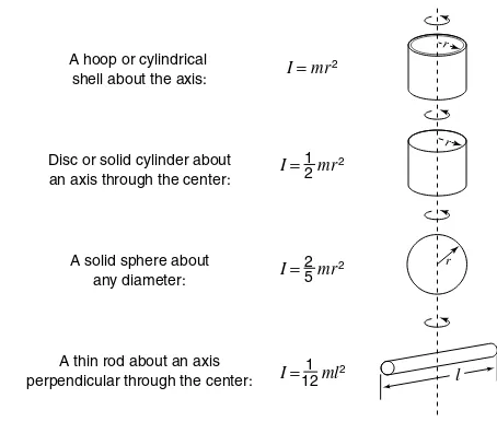
Moment of inertia . . . .38
Elasticity and Simple Harmonic Motion . . . .42
Elastic modules . . . .42
Hooke’s Law . . . .43
Simple harmonic motion . . . .43
The relation of SHM to circular motion . . . .44
The simple pendulum . . . .44
SHM energy . . . .45
Fluids . . . .45
Density and pressure . . . .45
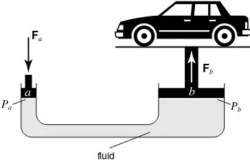
Pascal’s principle . . . .45
Archimedes’ principle . . . .46
Bernoulli’s equation . . . .47
Chapter 2: Waves and Sound . . . .49
Wave Motion . . . .49
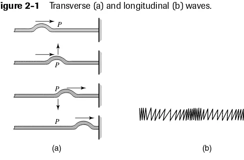
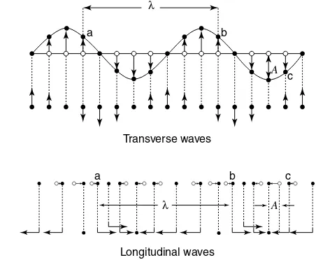
Transverse and longitudinal waves . . . .50
Wave characteristics . . . .50
Superposition principle . . . .52
Standing waves . . . .52
Sound . . . .53
Intensity and pitch . . . .54
Doppler effect . . . .54
Forced vibrations and resonance . . . .55
Beats . . . .56
Chapter 3: Thermodynamics . . . .58
Temperature . . . .58
Thermometers and temperature scales . . . .58
Thermal expansion of solids and liquids . . . .60
Development of the Ideal Gas Law . . . .61
Boyle’s law . . . .62
Charles/Gay-Lussac law . . . .62
Definition of a mole . . . .62
The ideal gas law . . . .62
Avogadro’s number . . . .63
The kinetic theory of gases . . . .63
Heat . . . .64
Heat capacity and specific heat . . . .64
Mechanical equivalent of heat . . . .65
Heat transfer . . . .65
Calorimetry . . . .66
Latent heat . . . .66
The heat of fusion . . . .67
The heat of vaporization . . . .67
The Laws of Thermodynamics . . . .69
The first law of thermodynamics . . . .69
Work . . . .70
Definitions of thermodynamical processes . . . .70
Carnot cycle . . . .71
The second law of thermodynamics . . . .73
Entropy . . . .74
Chapter 4: Electricity and Magnetism . . . .76
Electrostatics . . . .77
Electric charge . . . .77
Coulomb’s law . . . .79
Electric fields and lines of force . . . .80
Electric flux . . . .82
Gauss’s law . . . .83
Potential difference and equipotential surfaces . . . .84
Electrostatic potential and equipotential surfaces . . . .86
Capacitors . . . .89
Capacitance . . . .89
Parallel plate capacitor . . . .89
Parallel and series capacitors . . . .90
Current and Resistance . . . .92
Current . . . .92
Resistance and resistivity . . . .93
Electrical power and energy . . . .94
Direct Current Circuits . . . .94
Series and parallel resistors . . . .94
Kirchhoff’s rules . . . .96
Electromagnetic Forces and Fields . . . .97
Magnetic fields and lines of force . . . .98
Force on a moving charge . . . .98
Force on a current-carrying conductor . . . .100
Torque on a current loop . . . .100
Galvanometers, ammeters, and voltmeters . . . .101
Magnetic field of a long, straight wire . . . .101
Ampere’s law . . . .102
Magnetic fields of the loop, solenoid, and toroid . . . .103
Electromagnetic Induction . . . .103
Magnetic flux . . . .104
Faraday’s law . . . .104
Lenz’s law . . . .105
Generators and motors . . . .105
Mutual inductance and self-inductance . . . .106
Alternating Current Circuits . . . .107
Alternating currents and voltages . . . .107
Resistor-capacitor circuits . . . .108
Resistor-inductance circuits . . . .109
Reactance . . . .109
Resistor-inductor-capacitor circuit . . . .111
Power . . . .111
Resonance . . . .112
Transformers . . . .112
Chapter 5: Light . . . .114
Characteristics of Light . . . .114
Electromagnetic spectrum . . . .114
Speed of light . . . .115
Polarization . . . .116
Geometrical Optics . . . .118
The law of reflection . . . .118
Plane mirrors . . . .120
Concave mirrors . . . .121
Convex mirrors . . . .125
The law of refraction . . . .126
Brewster’s angle . . . .128
Total internal reflection . . . .128
Optical lenses . . . .129
The compound microscope . . . .131
Dispersion and prisms . . . .132
Wave Optics . . . .134
Huygens’ principle . . . .134
Interference . . . .134
Young’s experiment . . . .135
Diffraction . . . .136
Chapter 6: Modern Physics . . . .140
Relativity . . . .140
Frames of reference . . . .141
Michelson-Morley experiment . . . .141
The special theory of relativity . . . .142
Addition of velocities . . . .142
Time dilation and the Lorentz contraction . . . .143
The twin paradox . . . .144
Relativistic momentum . . . .144
Relativistic energy . . . .145
Quantum Mechanics . . . .147
Blackbody radiation . . . .147
Photoelectric effect . . . .147
Compton scattering . . . .149
Particle-wave duality . . . .149
De Broglie waves . . . .149
The Heisenberg uncertainty principle . . . .150
Atomic Structure . . . .150
Atomic spectra . . . .151
The Bohr atom . . . .151
Energy levels . . . .153
De Broglie waves and the hydrogen atom . . . .154
Nuclear Physics . . . .154
Nucleus structure . . . .154
Binding energy . . . .155
Radioactivity . . . .155
Half-life . . . .156
Nuclear reactions . . . .157
CQR Review . . . .159
CQR Resource Center . . . .166
Glossary . . . .168
P
hysics is a branch of physical science that deals with physical changes of objects. The mental, idealized models on which it is based are most frequently expressed in mathematical equations that simplify the condi-tion of the real world for ease of analysis. Even though the equacondi-tions are derived from ideal conditions, they approximate real situations closely enough to allow accurate prediction of the behaviors of complex systems. The primary task in studying physics is to understand its basic principles. Understanding these formal principles enables better understanding of the phenomena observed in the universe.The system of units used throughout this book is the International Sys-tem of Units (SI). This is the metric sysSys-tem, with which you may be famil-iar. The basic units are length (meter, m), mass (kilogram, kg), time (second, s), temperature (degrees celsius,°C, or Kelvin, K), electric current (amperes, A), and amount (mole). Standard prefixes are often used; for example, millimeter (10-3meter) is abbreviated mm. A list of the most commonly used prefixes is included in the Pocket Guide. Conversions between the fundamental units of the SI and the common American units (feet, pounds, and so on) are given on the Pocket Guide.
This book is written with a broad audience in mind. Therefore, concepts are presented at varying levels of mathematical sophistication. Each topic is generally first presented in a manner that requires only basic geometry and trigonometry. In some cases, formulae requiring knowledge of calcu-lus are given for those readers familiar with it. However, calcucalcu-lus is not required to understand the concepts in this book. In addition, some of the vector algebra and trigonometry used are presented in the first chapter and on the Pocket Guide.
Why You Need This Book
Can you answer yes to any of the following questions?
■ Do you need to review the fundamentals of physics quickly?
■ Do you need to prepare for your physics test?
■ Do you need a concise reference for physics?
If so, then CliffsQuickReview Physicsis for you!
How to Use This Book
You can use this book in any way that fits your personal style for study and review — you decide what works best with your needs. You can either read the book from cover to cover or just look for the information you want and put it back on the shelf for later. Here are a few recommended ways to search for topics.
■ Look for areas of interest in the book’s Table of Contents, or use the
index to find specific topics.
■ Flip through the book, looking for subject areas at the top of each
page.
■ Get a glimpse of what you’ll gain from a chapter by reading through
the “Chapter Check-In” at the beginning of each chapter.
■ Use the “Chapter Checkout” at the end of each chapter to gauge your
grasp of the important information you need to know.
■ Test your knowledge more completely in the CQR Review and look
for additional sources of information in the CQR Resource Center.
■ Use the glossary to find key terms fast. This book defines new terms
and concepts where they first appear in the chapter. If a word is bold-faced, you can find a more complete definition in the book’s glossary.
■ To get information quickly, check the Pocket Guide at the front of
the book.
■ Or flip through the book until you find what you’re looking for—we
Visit Our Web Site
A great resource, www.cliffsnotes.com, features review materials, valuable Internet links, quizzes, and more to enhance your learning. The site also features timely articles and tips, plus downloadable versions of many CliffsNotes books.
CLASSICAL MECHANICS
C h a p t e r C h e c k - I n
❑ Understanding motion (kinematics) in one and two dimensions, and
rotational motion
❑ Applying Newton’s Laws and analyzing force diagrams ❑ Using the concepts of energy and momentum
❑ Learning about periodic motion and elasticity ❑ Applying classical mechanics to fluids
M
echanics is the study of the motion of material objects. Classical orNewtonian mechanics deals with objects and motions familiar in our everyday world. Most people possess some intuition about classical mechanics; we all have watched a ball fly through the air or a bicycle tire spin. You should not be afraid to connect the formalism in this book with your intuition. Indeed, this is often the easiest way to see the answer to a difficult problem. Allow the formal physics and math to illuminate what you already know.Although textbook examples usually deal with blocks, springs, and other mundane devices, keep in mind that classical mechanics describes phe-nomena on a vast range of scales, from large molecules such as DNA to the planets of our solar system and beyond. In this chapter, you learn about the basic laws that these diverse systems all obey.
Kinematics in One Dimension
Definition of a vector
A vectoris a physical quantity with direction as well as magnitude, for
example, velocity or force. In contrast, a quantity that has only magnitude and no direction, such as temperature or time, is called a scalar.A vector is commonly denoted by an arrow drawn with a length proportional to the given magnitude of the physical quantity and with direction shown by the orientation of the head of the arrow.
Displacement and velocity
Imagine that a car begins traveling along a road after starting from a spe-cific sign post. To know the exact position of the car after it has traveled a given distance, it is necessary to know not only the miles it traveled but also its heading. The displacement, defined as the change in position of the object, is a vector with the magnitude as a distance, such as 10 miles, and a direction, such as east. Velocity is a vector expression with a magni-tude equal to the speed traveled and with an indicated direction of motion. For motion defined on a number line, the direction is specified by a pos-itive or negative sign. Average velocity is mathematically defined as
average
average velocityvelocity=totaltotal displacementtimetime elapseddisplacementelapsed
Note that displacement (distance from starting position) is notthe same as distance traveled. If a car travels one mile east and then returns one mile west, to the same position, the total displacement is zero and so is the aver-age velocity over this time period. Displacement is measured in units of length, such as meters or kilometers, and velocity is measured in units of length per time, such as meters/second (meters per second).
Average acceleration
Acceleration,defined as the rate of change of velocity, is given by the
fol-lowing equation:
average
average accelerationacceleration= finalfinal velocityvelocity initialtimetime elapsed-elapsedinitial velocityvelocity
Acceleration units are expressed as length per time divided by time such as meters/second/second or in abbreviated form as m s/ 2
Graphical interpretations of displacement, velocity, and acceleration
The distance versus time graph in Figure 1-1 shows the progress of a per-son: (I) standing still, (II) walking with a constant velocity, and (III) walk-ing with a slower constant velocity. The slope of the line yields the speed. For example, the speed in segment II is
((104 010 5-)m)s 45ms .8m s/
-= =
Figure 1-1 Motion of a walking person.
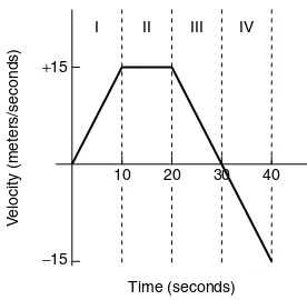
Each segment in the velocity versus time graph in Figure 1-2 depicts a different motion of a bicycle: (I) increasing velocity, (II) constant velocity, (III) decreasing velocity, and (IV) velocity in a direction opposite the initial direction (negative). The area between the curve and the time axis represents the distance traveled. For example, the distance traveled during segment I is equal to the area of the triangle with height 15 and base 10. Because the area of a triangle is (1/2)(base)(height), then (1/2)(15 m/s) (10 s) = 75 m. The magnitude of acceleration equals the calculated slope. The acceleration calculation for segment III is (–15 m/s)/(10 s) = –1.5 m/s/s or –1.5 m s/ 2
.
The more realistic distance-versus-time curve in Figure 1-3(a) illustrates gradual changes in the motion of a moving car. The speed is nearly con-stant in the first 2 seconds, as can be seen by the nearly concon-stant slope of the line; however, between 2 and 4 seconds, the speed is steadily decreas-ing and the instantaneous velocitydescribes how fast the object is mov-ing at a given instant.
4 8
5 10 15
Distance (meters)
Time (seconds) I
Figure 1-2 Accelerating motion of a bicycle.
Figure 1-3 Motion of a car: (a) distance, (b) velocity, and (c) acceleration change in time.
2 0 10 20 30 40 50 60
4 6 8 10 12 14
Distance (meters)
Time (seconds) (a)
2
−20
−15
−10
−5 0 5 10 15
4 6 8 10 12 14
V
elocity (meters/second)
Time (seconds) (b)
Time (seconds) (c) 2
−5
−10
−2.5 0 2.5
4 6 8 10 12 14
Acceler
ation (meters/second
2)
+15
10 20 30 40
−15
V
elocity (meters/seconds)
Time (seconds)
Instantaneous velocity can be read on an odometer in the car. It is calcu-lated from a graph as the slope of a tangent to the curve at the specified time. The slope of the line sketched at 4 seconds is 6 ms. Figure 1-3(b) is a sketch of the velocity-versus-time graph constructed from the slopes of the distance-versus-time curve. In like fashion, the instantaneous
accel-erationis found from the slope of a tangent to the velocity-versus-time
curve at a given time. The instantaneous acceleration-versus-time graph in Figure 1-3(c) is the sketch of the slopes of the velocity-versus-time graph of Figure 1-3(b). With the vertical arrangement shown, it is easy to com-pute the displacement, velocity, and acceleration of a moving object at the same time.
For example, at time t= 10 s, the displacement is 47 m, the velocity is –5 m/s, and the acceleration is 5m s/ 2
- .
Definitions of instantaneous velocity and instantaneous acceleration
The instantaneous velocity, by definition, is the limit of the average veloc-ity as the measured time interval is made smaller and smaller. In formal terms, v=limlim∆t"0∆d ∆t. The notation limlim∆t"0 means the ratio ∆d ∆tis evaluated as the time interval approaches zero. Similarly, instantaneous acceleration is defined as the limit of the average acceleration as the time interval becomes infinitesimally short. That is, a=limlim∆t"0∆v ∆t.
Motion with constant acceleration
When an object moves with constant acceleration, the velocity increases or decreases at the same rate throughout the motion. The average acceler-ation equals the instantaneous acceleracceler-ation when the acceleracceler-ation is con-stant. A negative acceleration can indicate either of two conditions:
■ Case 1: The object has a decreasing velocity in the positive direction.
■ Case 2: The object has an increasing velocity in the negative
direction.
Using vo(velocity at the beginning of time elapsed), vf(velocity at the end of the time elapsed), and tfor time, the constant acceleration is
a vf t vo oror v v atat
f o
= - = + [Equation 1]
Substituting the average velocity as the arithmetic average of the original and final velocities vavgavg=(vo+vf)/)/2into the relationship between distance
and average velocity d=(vavgavg)()( )t yields )t
(
d= 21 vo+vf [Equation 2] Substitute vffrom Equation 1 into Equation 2 to obtain
d v t= o +21atat2 [Equation 3]
Finally, substitute the value of tfrom Equation 1 into Equation 2 for
vf vo 2adad
2 2
= + [Equation 4]
These four equations relate v vo, f, t, a, and d. Note that each equation has a different set of four of these five quantities. Table 1-1 summarizes the equations for motion in a straight line under constant acceleration. A special case of constant acceleration occurs for an object under the influ-ence of gravity. If an object is thrown vertically upward or dropped, the acceleration due to gravity of 9 8. m s/2
- is substituted in the above equa-tions to find the relaequa-tionships among velocity, distance, and time.
Table 1-1 Equations and Variables of Kinematics in One Dimension
Information Given Variables
Equation by Equation vo vf t a d
vf=vo+atat Velocity as a function of time ✓ ✓ ✓ ✓ X
( )
d= 21 vo+v tf Displacement varying with ✓ ✓ ✓ X ✓ velocity and time
d v t= o +21atat2 Displacement as a function ✓ X ✓ ✓ ✓
of time
vf vo 2adad
2 2
= + Velocity as a function ✓ ✓ X ✓ ✓
of displacement
Kinematics in Two Dimensions
analysis, many motions can be simplified to two dimensions. For example, an object fired into the air moves in a vertical, two-dimensional plane; also, horizontal motion over the earth’s surface is two-dimensional for short dis-tances. Elementary vector algebra is required to examine the relationships between vector quantities in two dimensions.
Addition and subtraction of vectors: geometric method The vector Ashown in Figure 1-4(a) represents a velocity of 10 m/s north-east, and vector Brepresents a velocity of 20 m/s at 30 degrees north of east. (A vector is named with a letter in boldface,nonitalic type, and its magnitude is named with the same letter in regular, italictype. You will often see vectors in the figures of the book that are represented by their magnitudes in the mathematical expressions.) Vectors may be moved over the plane if the represented length and direction are preserved.
Figure 1-4 Graphical addition of vectors, A + B = C.
In Figure 1-4(b), the same vectors are positioned to be geometrically added. The tail of one vector, in this case A, is moved to the head of the other vec-tor (B). The vector sum (C) is the vector that extends from the tail of one vector to the head of the other. To find the magnitude of C,measure along its length and use the given scale to determine the velocity represented. To find the direction θof C,measure the angle to the horizontal axis at the
tail of C.
Figure 1-5(a) shows that A +B =B +A.The sum of the vectors is called
the resultantand is the diagonal of a parallelogram with sides AandB.
Figure 1-5(b) illustrates the construction for adding four vectors. The result-ant vector is the vector that results in the one that completes the polygon.
1 cm = 5 m/s (a) 45° A
30° B
1 cm = 5 m/s (b)
θ
45° A
30° B
Figure 1-5 (a) A +B =B +A. (b) Graphical addition of several vectors.
To subtract vectors, place the tails together. The difference of the two vec-tors (D) is the vector that begins at the head of the subtracted vector (B) and goes to the head of the other vector (A). An alternate method is to add the negative of a vector, which is a vector with the same length but pointing in the opposite direction. The second method is demonstrated in Figure 1-6.
Figure 1-6 Graphical subtraction of vectors, A –B =D.
Addition and subtraction of vectors: Component method
For precision in adding vectors, an analytical method using basic trigonom-etry is required because scale drawings do not give accurate values. Consider vector Ain the rectangular coordinate system of Figure 1-7. The vector Acan be expressed as the sum of two vectors along the xand yaxes, A=Ax+Ay,where Axand Ayare called the componentsof A. The direc-tion of Ax is parallel to the xaxis, and that of Ayis parallel to the yaxis.
A
D −B
B
(a)
A
A R=
A+ B
B B
(b)
A
B C D
R= A
+B +C
The magnitudes of the components are obtained from the definitions of the sine and cosine of an angle: coscosθ=A Ax/ and sinsinθ=A Ay/ , or
cos cos sin sin
A A
A A
θ
θ
x
y
=
=
Figure 1-7 Components of a vector.
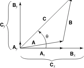
To add vectors numerically, first find the components of all the vectors. The signs of the components are the same as the signs of the cosine and sine in the given quadrant. Then, sum the components in the xdirection, and sum the components in the ydirection. As shown in Figure 1-8, the sum of the
xcomponents and the sum of the ycomponents of the given vectors (Aand
B) comprise the xand ycomponents of the resultant vector (C).
These resultant components form the two sides of a right angle with a hypotenuse of the magnitude of C; thus, the magnitude of the resultant is
y x
C C2 C2
= +
Figure 1-8 Component method of vector addition, A+ B= C.
Ax Bx
B
A C By
Cy
Cx Ay
θ
A
Ax Ay
O
y
x
tanθ= Ax Ay
The direction of the resultant (C) is calculated from the tangent because y
x /
tan
tanθ=C C . To solve for the angle θ, use θ=tantan-1(C Cy/ x .) The procedure can be summarized as follows:
1. Sketch the vectors on a coordinate system.
2. Find the xand ycomponents of all the vectors, with the
appro-priate signs.
3. Sum the components in both thexand ydirections.
4. Find the magnitude of the resultant vector from the
Pythagorean theorem.
5. Find the direction of the resultant vector using the tangent
function.
Follow the same procedure to subtract vectors by calculating the appro-priate algebraic sum of the components in Step 3.
Multiplication of vectors
The dot product: There are two different ways in which two vectors may
be multiplied together. The first is the dot product, also called the scalar product, which is written A ⋅ B. This can be evaluated in two ways:
■ A⋅B = A
xBx+ AyBy
■ A⋅B = AB cos θ, where θis the angle between the vectors when they
are set tail to tail, and Aand Bare the lengths of the vectors.
Note that the order of the vectors does not matter and that the result of the dot product is a scalar rather than a vector. Note that if two vectors are per-pendicular, their dot product is zero according to the second rule above.
Cross product: The second way to multiply vectors is called the cross
productor the vector product. It is written A ⋅ B. It can be evaluated in
two ways:
■ A⋅ B = (A
xBy– AyBx)z,when the vectors Aand Bboth are in x-yplane.
The zindicates that the result is a vector that points along the zaxis. In general, the vector resulting from a cross product is always per-pendicular to both of the vectors being multiplied together.
■ A⋅ B = ABz sin θ, where θis the angle between the vectors Aand B
when they are placed tail to tail. Again, the result is a vector perpen-dicular to Aand B(and therefore points along the zaxis if Aand B
The result of a cross product does depend on the order of the vectors. Note from the first rule that A⋅ B = –B ⋅A. Also, if Aand Bare parallel, the second rule implies that their cross product is zero.
Finally, the cross product give rise to the “right hand rule,” which allows you to easily determine the direction of the resulting vector. For the gen-eral expression A×B= C, point your thumb in the direction of A.Now point your index finger in the direction of B; if necessary, flip over your hand. The vector C points outward from your palm. For an illustration of this procedure, flip ahead to Chapter 4 (Figure 4-19), where the rule is applied to the equation F= qv×B.
Velocity and acceleration vectors in two dimensions For motion in two dimensions, the earlier kinematics equations must be expressed in vector form. For example, the average velocity vector is
( ) t
v= df-do , where doanddf are the initial and final displacement
vec-tors and tis the time elapsed. As noted earlier, the velocity and displace-ment vectors are shown in bold type, whereas the scalar (t)is not. In similar fashion, the average acceleration vector is a=(vf-vo) t, where voand vf
are the initial and final velocity vectors.
An important point is that the acceleration can arise from a change in the magnitude of the velocity (speed) as well as from a change in the direction of the velocity. If an object travels around a circle at a constant speed, there is an acceleration due to the change in the direction of the velocity, even though the magnitude of the velocity does not change. A mass moves in a horizontal circle with a constant speed in Figure 1-9. The velocity vectors at positions 1 and 2 are subtracted to find the average acceleration, which is directed toward the center of the circle. (Note that the average accelera-tion vector is placed at the midpoint of the path in the given time interval.)
Figure 1-9 Velocity and acceleration vectors of an object moving in a circle.
v2
2
a
(a) (b)
1 v1
v2 a
The following discussion summarizes the four different cases for acceler-ation in a plane:
■ Case 1: Zero acceleration
■ Case 2: Acceleration due to changing direction but not speed
■ Case 3: Acceleration due to changing speed but not direction
■ Case 4: Acceleration due to changing both speed and direction.
Imagine a ball rolling on a horizontal surface that is illuminated by a stro-boscopic light. Figure 1-10(a) shows the position of the ball at even inter-vals of time along a dotted path. Case 1 is illustrated in positions 1 through 3; the magnitude and direction of the velocity do not change (the pictures are evenly spaced and in a straight line), and therefore, there is no acceler-ation. Case 2 is indicated for positions 3 through 5; the ball has constant speed but changing direction, and therefore, an acceleration exists. Figure 1-10(b) illustrates the subtraction of v3and v4and the resulting accelera-tion toward the center of the arc. Case 3 occurs from posiaccelera-tions 5 to 7; the direction of the velocity is constant, but the magnitude changes. The accel-eration for this portion of the path is along the direction of motion. The ball curves from position 7 to 9, showing case 4; the velocity changes both direction and magnitude. In this case, the acceleration is directed nearly upward between 7 and 8 and has a component toward the center of the arc due to the change in direction of the velocity and a component along the path due to the change in the magnitude of the velocity.
Figure 1-10 (a) Path of a ball on a table. (b) Acceleration between points 3 and 4.
(a) (b)
v3
v3
v4
v4 a
1 2
3 4
5 6 7
Projectile motion
Anyone who has observed a tossed object—for example, a baseball in flight—has observed projectile motion. To analyze this common type of motion, three basic assumptions are made: (1) acceleration due to gravity is constant and directed downward, (2) the effect of air resistance is negli-gible, and (3) the surface of the earth is a stationary plane (that is, the cur-vature of the earth’s surface and the rotation of the earth are negligible). To analyze the motion, separate the two-dimensional motion into vertical and horizontal components. Vertically, the object undergoes constant accel-eration due to gravity. Horizontally, the object experiences no accelaccel-eration and, therefore, maintains a constant velocity. This velocity is illustrated in Figure 1-11 where the velocity components change in the ydirection; how-ever, they are all of the same length in the xdirection (constant). Note that the velocity vector changes with time due to the fact that the vertical com-ponent is changing.
Figure 1-11 Projectile motion.
In this example, the particle leaves the origin with an initial velocity ( )vo , up at an angle of θo. The original xand ycomponents of the velocity are
given by vxoxo=vo coscosθoand vyoyo=vo sinsinθo.
θ
0
y
x
vy0
vx 0
vx0
vx 0 vx0
v0
v
v g
vy
vy
vy= 0
vx0
vy= −vy0
θ
θ
With the motions separated into components, the quantities in the xand
ydirections can be analyzed with the one-dimensional motion equations subscripted for each direction: for the horizontal direction, vx=vxoxoand
x v t= xoxo ; for vertical direction, vy=vyoyo-gtgtand y v t= yoyo -`1 2jgtgt2, where x and yrepresent distances in the horizontal and vertical directions, respec-tively, and the acceleration due to gravity ( g )is 9 8. m s/ 2
. (The negative sign is already incorporated into the equations.) If the object is fired down at an angle, the ycomponent of the initial velocity is negative. The speed of the projectile at any instant can be calculated from the components at that time from the Pythagorean theorem, and the direction can be found from the inverse tangent on the ratios of the components:
1
-x
tan tan
v v v
v v
θ
y
y x
= +
=
2 2
d n
Other information is useful in solving projectile problems. Consider the example shown in Figure 1-11 where the projectile is fired up at an angle from ground level and returns to the same level. The time for the projec-tile to reach the ground from its highest point is equal to the time of fall for a freely falling object that falls straight down from the same height. This equality of time is because the horizontal component of the initial velocity of the projectile affects how far the projectile travels horizontally but not the time of flight. Projectile paths are parabolic and, therefore, symmetric. Also for this case, the object reaches the top of its rise in half of the total time (T)of flight. At the top of the rise, the vertical velocity is zero. (The acceleration is always g, even at the top of the flight.) These facts can be used to derive the rangeof the projectile, or the distance traveled horizontally. At maximum height, vy=0 and t =T/2; therefore, the
velocity equation in the vertical direction becomes 0=vosinsinθ-g T/2or
solving for T, T=(2vo sinsinθ)/)/g.
Substitution into the horizontal distance equation yields R=(vo coscosθ)T.
Substitute T in the range equation and use the trigonometry identity
sin
sin2θ=2sinsinθ coscosθto obtain an expression for the range in terms of the initial speed and angle of motion, R ( / ) sinv g sin2θ
o
2
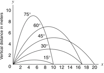
Figure 1-12 Range of projectiles launched at different angles.
Uniform circular motion
For uniform motion of an object in a horizontal circle of radius (R), the con-stant speed is given by v=2πR T/ , which is the distance of one revolution
divided by the time for one revolution. The time for one revolution (T)is defined as period.During one rotation, the head of the velocity vector traces a circle of circumference 2πvin one period; thus, the magnitude of the accel-eration is a=2πv T/ . Combine these two equations to obtain two additional
relationships in other variables: a v R2/
= and a=^4π2/T R2h .
The displacement vector is directed out from the center of the circle of motion. The velocity vector is tangent to the path. The acceleration vec-tor directed to the center of the circle is called centripetal acceleration. Figure 1-13 shows the displacement, velocity, and acceleration vectors at different positions as the mass travels in a circle on a frictionless horizon-tal plane.
Figure 1-13 Uniform circular motion.
v1 v2
d2
d1 a1 a2
y
x
0 2 4 6 8
Range in meters (horizontal distance)
V
er
tical distance in meters
10 12 14 16 18 20 2
4 6 8 10
75°
60°
45°
30°
Dynamics
The study of dynamics goes beyond the relationships between the vari-ables of motion as illuminated in kinematics to the cause of motion, which is force.
Newton’s laws of motion
Newton’s first law of motion,also called the law on inertia, states that an
object continues in its state of rest or of uniform motion unless compelled to change that state by an external force. The law appears to contain two separate statements. The first statement—that a state of rest will con-tinue unless a force is applied—seems intuitively correct. The second state-ment—that an object will continue with a constant velocity unless compelled to change by an impressed force—seems contrary to common experience. It is important to realize that objects observed to slow down are being compelled to change by a frictional force. Frictionis a retarding force that is ever present in our everyday world. For the ideal—the absence of outside forces acting on the object, as described by the law—friction must be eliminated. The value of the law is the introduction of the con-cept of forceas a push or pull that causes a body to change its state of motion.
Newton’s second law of motionstates that if a net force acts on an object,
it will cause an acceleration of that object. The law addresses the cause and effect relationship between force and motion commonly stated as F= ma,
where mis the proportionality constant (mass). Force is measured in SI units of newtons,abbreviated N.
Newton’s third law of motionstates that for every action there is an equal
and opposite reaction. Therefore, if one object exerts a force on a second object, the second exerts an equal and oppositely directed force on the first one.
Mass and weight
Massand weightare distinctly different physical quantities, a fact that
cannot be emphasized too strongly. Mass is the property that lends an object a reluctance to change its state of motion. Mass is the measure of the amount of matter in an object. Masses are compared on an equal-arm balance. If a loaded two-pan balance is level on earth, it will be level in a different gravitational field, as for example, on the moon. Thus, mass is an invariant quantity; it is measured in units of kilograms. A mass of 1 kilogram will experience an acceleration of 1m s/ 2
The force that the earth exerts on an object of specific mass is called the object’s weight on earth. Weight is a force measured in units of newtons and is a vector quantity. The expression for weight is W= mg, where gis the acceleration due to gravity. A spring scale translates the force of attrac-tion between an object and the earth into a reading of weight. In contrast to a measurement of mass, weight is not an invariant. An object on a spring scale on earth would not weigh the same on the moon because the pull of gravity on the object differs in the two locations.
Force diagrams
To better understand the relationship between force and acceleration in a particular case, it is helpful to use a force diagram,also called a free-body
diagram.An object that is not moving is said to be in a static
equilib-rium.An example is a weight hanging by two ropes from the ceiling (see
Figure 1-14). To analyze this problem, consider the forces acting on the knot joining the ropes. Then,
1. Make the force diagram.
2. Find the components of forces not directed along the
coordi-nate axes and write the force equation for each axis.
3. Solve the simultaneous equations for the tensions.
The following examples illustrate these procedures. (All of the following vector diagrams are drawn to scale.)
Example 1: What is the tension in each rope in Figure 1-14?
Figure 1-14 Force diagram of a suspended weight.
1. Make the force diagram.
The tension in the lower rope attached to the mass must be mg
directed downward; therefore, T3= -mgmg.
T1
45° 45°
T3 W
(b) T2
45°
2. Find the components of forces not directed along the coordi-nate axes and write the force equation for each axis.
Components of the forces in the xdirection are
% %
cos
cos coscos
T2 4545 -T1 4545 =0
Components of the forces in the y direction are
% %
sin
sin sinsin
T2 4545 +T1 4545 -mgmg=0
3. Solve the simultaneous equations for the tensions.
Solution:T T mgmg 2
1= 2=
To minimize computation errors, show the components on a separate force diagram as shown in Figure 1-14.
Example 2: Now, see if you can make the free-body diagram and set up
the force equations for a pail on the end of a rope that is accelerating upward. Find the tension in the rope and the acceleration of the pail. See Figure 1-15(a).
Figure 1-15 Force diagram of a bucket being lifted.
The two forces acting on the pail are the tension of the rope (T) and weight (W = mg). By Newton’s second law:
Solution:Fnetnet=T-mgmg ma=ma
Example 3:Next, try to set up the equations for a two-body system
of unequal masses attached by a rope over a frictionless pulley (see Figure 1-16). A diagram must be made for each of the two objects of mass
(m1)and (m2). Find the acceleration of the system and the tension in the rope.
(b) T
W
(a)
Figure 1-16Force diagram of two masses hung over a pulley.
: ,
: ,
m F T m g m a
m T m g m a
For
For asas magnitudesmagnitudes
For
For asas magnitudesmagnitudes
net net
1 1 1
2 2 2
= - =
- =
-The second equation has a negative acceleration because m2is descending. Because the objects are connected by a rope that does not expand, the ten-sions and accelerations are the same for each mass. By algebraic manipu-lation, the equations may be simultaneously solved for the following results:
Solution:a mm22 mm11 g andandT m2m m gm
1 2 1 2
= +- = +
Example 4:In Figure 1-17, one object sits on a frictionless surface, and
the other object hangs off the edge of the table over a pulley. Make the free-body diagram and write the force equations to find the acceleration and tension.
Figure 1-17 Same as Figure 1-16 with one mass on a frictionless table.
In the vertical direction, the forces on mare the weight downward and the normal force (N) upward due to the surface, which is equal and opposite to the weight. Because there is no acceleration ofm1 in this direction, the net vertical force is zero. A horizontal force of the tension in the rope accel-erates the mass to the right. Write the force equations separately for xand
N T
(a) (b)
m1
m2
m1g m1a
m2g a
T T
a
(a) (b)
m1
m2
m2 > m1
m1g
ydirections for m1. The forces on the second mass are the same as those in the last example. For m1in thexdirection: T m a= 1 ; in the ydirection:
N-m g1 =0. For m2: T-m g2 = -m a2 . Combining the two equations gives the relationships.
Solution:a m1m2m2 g andandT mm mm g
1 2 1 2
= + = +
Even more complicated problems can be separated into manageable parts to allow solution by using these problem-solving methods.
Example 5: Consider a mass (m1)on an inclined plane attached to a mass
(m2)over a pulley as in Figure 1-18(a). Both the plane and pulley are
fric-tionless. Set up the problem to find the acceleration.
Figure 1-18 Now the table in Figure 1-17 is tilted at an angle.
In this case, the forces on m1must be resolved in components along the x and yaxes. The coordinate system with the xaxis parallel to the surface of the plane is selected so that only one force, the weight of m1, needs to be converted into component form. The normal force is always perpendicu-lar to the plane and in this case, therefore, is opposed only be the compo-nent of weight that is also perpendicular to the plane’s surface. Note that the angle between the yaxis and the weight (m1g) is the angle of inclina-tion of the plane, which can be proven by geometry. The coordinate sys-tem for m2has the same orientation as in the previous example. Assume
>
m2 m1. Then, for m1in its ydirection: N-m g1 coscosθ=0; in its x direc-tion: T-m g1 sinsinθ=m a1 . For m T2: -m g2 = -m a2 . The acceleration is then
Solution:a=(m2-mm1+1 msinsin2θ)g
and tension is T=(1+sinsinm1+θ)mm m g21 2
N T
T
(a) (b)
m1
m2
y x
y x
m1g
m2g m2 > m1
θ
To analyze a physical situation by the use of free-body diagrams, use the following steps:
1. Make a free-body diagram for each object.If one object is sitting
on a surface, be sure to include the normal force.
2. Resolve the forces that are not directed along the x and y axes
into components along a preferred coordinate system.For
inclined planes, use a coordinate axis with the xaxis parallel to the surface of the plane. Put the components on a separate diagram; that is, do not put the force and its components on the same diagram because this combination might complicate the following steps.
3. Write out the force equation for each mass along each axis,
not-ing the correct sign for the acceleration of the body.
4. Solve the equations simultaneously to find the desired
value(s).
Friction
Frictionis the force opposing the motion of one body sliding or rolling
over the surface of second object. Several aspects of friction are important at low velocities:
■ The direction of the force of friction is opposite the direction of
motion.
■ The frictional force is proportional to the perpendicular (normal)
force between the two surfaces in contact.
■ The frictional force is nearly independent of the area of contact
between the two objects.
■ The magnitude of the frictional force depends on the materials
com-posing the two objects in contact.
Static frictionis the force of friction when there is no relative motion
between two objects in contact, such as a block sitting on an inclined plane. The magnitude of the frictional force is Fs#µsN, where Nis the
Kinetic frictionis the force of friction when there is relative motion between two objects in contact. The magnitude of the friction force in this case is Fk#µkN, where Nis the magnitude of the normal force and µkis the coefficient of kinetic friction. Note that µkis not strictly a constant, but this empirical rule is a good approximation for finding frictional forces. Values given for the coefficients of static and kinetic friction do vary with speed and surface conditions so that it is not necessarily true that static friction exceeds sliding friction.
The following problem highlights the differences between static and kinetic friction.
Example 6:A block sits on an inclined plane. What is the maximum angle
that which the block remains at rest? First, draw the free-body diagrams and then write out the force equation for each direction of the coordinate system (see Figure 1-19).
Figure 1-19 A block on an inclined plane, with friction.
Suppose the surface is tilted to θ, at which the block just begins to
move. Then, the force down the plane must be equal to the maximum force of static friction; thus f frictionfriction=µsN. Therefore,
( )
sin
sin coscos
ffrictionfriction=mgmg θ=µsN=µs mgmg θ and solving for the coefficient of friction:
Solution:µs=tantanθ
At a greater angle of tilt, the object accelerates down the surface, and the force of friction is fk=µkN.
Example 7:If the surfaces in Figures 1-17 and 1-18 were notfrictionless,
the frictional force parallel to the surface and opposite the direction of
N
ffriction
(a) (b)
m1
mg
N−mg cosθ= 0
mg sinθ = ffriction
θ
motion must be included in the analysis. Pulling a block along a horizon-tal surface at a constant speed (zero acceleration) is an example of a prob-lem involving friction, and such a block is analyzed in Figure 1-20.
Figure 1-20 Pulling a block on a plane with friction.
In the xdirection, Tcoscosθ- =f 0, where fis the friction force and Tis the
tension in the rope. In the ydirection, N+Tsinsinθ-mgmg=0; also, f=µkN. Solve the ydirection equation for N, substitute the expression into the fric-tion force equafric-tion, and then substitute fricfric-tion into the first equafric-tion to obtain the following:
( )
cos
cos sinsin
T θ-µk mgmg-T θ =0
Solution:T=coscosθµkmgmgµ sinsinθ
+ , solving for T.
Centripetal force
When an object rotates in a circle, a force must be directed to the center of the circle to maintain the motion; otherwise, the object will take off tangent to the path. This constraining force is called a centripetal force,
meaning center-seeking. In the example of a mass rotating in a horizontal circle at the end of the string, the centripetal force is provided by the ten-sion in the string. In the case of orbiting satellites, gravity provides the center-seeking force. From the definition of force F= maand the expres-sions for circular accelerations, the following equations are obtained:
F m Rv F m Tv F
T
m R
or
or 2π oror 4π
c c c
2
2 2
= = =
-If an object moves in a circle, the net force is a centripetal force. One such example is the conic pendulum, a mass on the end of a string that rotates in a horizontal circle (see Figure 1-21).
T
(a) (b)
mg
m
θ θ
Figure 1-21 A conic pendulum.
In the ydirection, T coscosθ-mgmg=0. In the xdirection (or the radial
direc-tion), T sinsinθ=mvmv R2/ , where Ris the radius of circular path. Dividing the
second equation by the first equation and solving for vyields the following:
cos cos sin sin
tan tan
v= gRgR θθ = gRgR θ
Universal gravitation
Newton’s law of universal gravitationstates that every mass in the
uni-verse attracts every other mass with a gravitational force that is directly pro-portional to the product of their masses ( ,m m1 2)and inversely proportional
to the square of distance (r) between them. In mathematical form,
( )/)/
F= GmGm m1 2 r2, where Gis the universal gravitational constant.In the
metric system, the accepted value of G isisG 6 673.673 1010 1111(NmNm kg2/kg2) #
= - .
Kepler found three empirical laws regarding the motion of satellites that Newton later showed from his law of universal gravitation. These are
Kepler’s laws of planetary motion:
■ The law of orbits: All planets move in elliptical orbits with the sun
at one focus.
■ The law of areas: A line joining a planet and the sun sweeps out equal
areas in equal time.
■ The law of periods:The square of the period (T)of any planet is
proportional to the cube of the semi-major axis (r) of its orbit, or
( /
T2 4π2 GMGM 3
= )r , where Mis the mass of the planet.
T
bob
L
R
m
(a) (b)
W(=mg)
y
θ
Momentum and impulse
According to Newton’s second law, a mass experiencing a net average force (F) for a time interval ∆twill undergo an average acceleration (F=ma). The product of the average force acting on the body and time of contact is defined as impulse. Because acceleration is change in velocity, the relationships between these variables are expressed as the
( )t m m
Impulse
Impulse=F ∆ = vf- vi, where viis the initial velocity and vf is the
velocity after the force is no longer in contact with the body. Impulse is measured in units of newton-seconds, or more simply, N-s.
When applying the impulse equation, be sure to calculate the vector change in velocity—for example, consider a mass of 10 kg acted on by a force that changes its velocity from –8 m/s to 3 m/s . This force imparted an impulse of (10 kg)[3 – (–8) m/s] = (10 kg)(11 m/s) = 110 N-s.
The right side of the impulse equation is the change in the linear momen-tumof the object. The definition of linear momentum is p= mv. Linear momentum is measured in units of kilogram meters/second or, in abbre-viated form, kg m/s. Newton originally stated his second law by saying that the rate of change of momentum with time is proportional to the impressed force and is in the same direction; thus, F=∆( )/mv)/∆t ororF=∆ ∆p/ t.
Conservation of momentum
An extremely important fundamental principle in physics is the law of
con-servation of momentum. The law states that if there is no external force
Another way to state the law of conservation of momentum is that the change in momentum of the two objects must be equal and opposite. For example, two ice skaters are at rest in the center of frictionless ice (possi-ble at least in the imagination). Let one have a relatively small mass (m)
and the other a larger mass (M). Because they begin at rest, the initial momentum is zero. They then push apart in opposite directions. The total momentum must remain zero.
According to the law of conservation of momentum, ∆pm= -∆pM or
( )
mvl-0=-MVl-0; therefore, if the large mass (M)is three times the
smaller mass (m), vl= -3Vl, where vlis the velocity of the small mass after the collision and Vlis the velocity of the large mass after the collision. The negative sign indicates velocities in opposite directions.
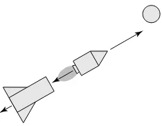
This same analysis holds for a person standing on frictionless ice who throws an object; it even holds for a rocket going to the moon. The ice skater throwing a glove attains equal momentum in the direction oppo-site to that of the thrown object. This basic principle is the same for a rocket accelerating in space. Spacecrafts utilize the law of conservation of momentum in getting an additional push from discharged rocket stages as well as from fuel. In particular, the Apollo space capsule returning from the moon was only a small percent of the total mass initially sent upward from the launch pad; therefore, acceleration of a rocket can be caused by either a change in velocity, by a change in its mass, or by changes in both velocity and mass (see Figure 1-22). Thus, the expression of Newton’s sec-ond law of motion, stated in terms of the change of momentum, is broader than the expression given only in terms of mass and acceleration.
Figure 1-22 A rocket ship gains momentum.
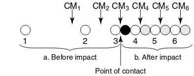
If two objects strike with a glancing blow, the motion will be two-dimensional. For example, one ball (m1)with an initial velocity hits a
second ball (m2), which is initially at rest. Figures 1-23 and 1-24 depict this
The momentum vectors can be added to show the law of conservation of momentum. The vector addition in Figure 1-24(a) shows that the total of the two momentum vectors, p1'and p2', after the collision are equal to the total momentum before the collision. (Because only m1was moving, there was only one initial momentum vector, p1.) Figure 1-24(b) also shows the alternate method of using the law of conservation of momentum, that the change (difference) in momentum of m1is equal and opposite to that of m2.
Figure 1-23 Two balls striking a glancing blow.
Figure 1-24 (a) Total momentum is conserved. (b) Equal and opposite momentum changes of the two balls.
(a) (b)
If the two masses are not equal, the velocity vectors must be adjusted so that the vectors represent momentum. For example, if one mass is three times the other, the velocity vectors of the larger mass must be lengthened by a factor of three before using the law of conservation of momentum.
p1= p1′ + p2′
p2′ = ∆p2
p1′− p1 = ∆p1
p1
p1′
p1
p1′
p1
p1′
p2′
Work and Energy
The concepts of work and energy are closely tied to the concept of force because an applied force can do work on an object and cause a change in energy. Energyis defined as the ability to do work.
Work
The concept of work in physics is much more narrowly defined than the common use of the word. Workis done on an object when an applied force moves it through a distance. In our everyday language, work is related to expenditure of muscular effort, but this is notthe case in the language of physics. A person that holds a heavy object does no physical work because the force is not moving the object through a distance. Work, according to the physics definition, is being accomplished while the heavy object is being lifted but not while the object is stationary. Another exam-ple of the absence of work is a mass on the end of a string rotating in a horizontal circle on a frictionless surface. The centripetal force is directed toward the center of the circle and, therefore, is not moving the object through a distance; that is, the force is not in the direction of motion of the object. (However, work was done to set the mass in motion.) Mathematically, work is W=F x$ , where Fis the applied force and xis the
distance moved, that is, displacement. Work is a scalar. The SI unit for work is the joule (J), which is newton-meter or kg m s/ 2.
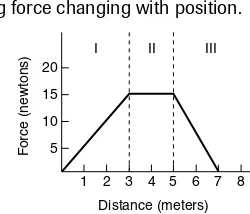
If work is done by a varying force, the above equation cannot be used. Figure 1-25 shows the force-versus-displacement graph for an object that has three different successive forces acting on it. The force is increasing in segment I, is constant in segment II, and is decreasing in segment III. The work performed on the object by each force is the area between the curve and the xaxis. The total work done is the total area between the curve and the xaxis. For example, in this case, the work done by the three successive forces is shown in Figure 1-25.
Figure 1-25 Acting force changing with position.
5 10 15 20
2 4 6 8
1 3 5 7
F
orce (ne
wtons)
Distance (meters)
In this example, the total work accomplished is (1/2)(15)(3) + (15)(2) + (1/2)(15)(2) = 22.5 + 30 + 15; work = 67.5 J. For a gradually changing force, the work is expressed in integral form, W=
#
F$dx.Kinetic energy
Kinetic energyis the energy of an object in motion. The expression for
kinetic energy can be derived from the definition for work and from kine-matic relationships. Consider a force applied parallel to the surface that moves an object with constant acceleration.
From the definition of work, from Newton’s second law of motion, and from kinematics, W Fx=Fx max=maxand vf =vo +2axax
2
2 , or
f o
( )/)/
a= v2-v2 2x. Substitute
the last expression for acceleration into the expression for work to obtain
f o
( )/)/
W m v= 2-v2 2or W=( / )1 2 mvmvf -( / )1 2 mvmvo )
2
2 . The right side of the last
equation yields the definition for kinetic energy: K E. . ( / )= 1 2 mvmv2. Kinetic
energy is a scalar quantity with the same units as work, joules (J). For exam-ple, a 2 kg mass moving with a speed of 3 m/s has a kinetic energy of 9 J. The above derivation shows that the net work is equal to the change in kinetic energy. This relationship is called the work-energy theorem:
. . . .
Wnetnet=K Ef -K Eo, where K E. .f is the final kinetic energy and K E. .ois the original kinetic energy.
Potential energy
Potential energy,also referred to as stored energy, is the ability of a
sys-tem to do work due to its position or internal structure. Examples are energy stored in a pile driver at the top of its path or energy stored in a coiled spring. Potential energy is measured in units of joules.
Gravitational potential energyis energy of position. First, consider
gravitational potential energy near the surface of the earth where the acceleration due to gravity (g)is approximately constant. In this case, an object’s gravitational potential energy with respect to some reference level is P.E. = mgh, where his the vertical distance above the reference level. To lift an object slowly, a force equal to its weight (mg)is applied through a height (h). The work accomplished is equal to the change in potential energy: W P E= . .f-P E. .o=mghmghf-mghmgho, where the subscripts (fand o)refer to the final and original heights of the body.
gis not constant. The general form of gravi