A MODEL FOR STATIC AND DYNAMIC
PHENOMENA IN DEPOSITION PROCESSES
M. Hasan and J.H.J. van Opheusden
Abstract.We have developed a model for friction in a dry granular material, that allows multiple reversible transitions between stick and slip contacts. The ultimate purpose of the model is to simulate deposition processes. During these processes a pile structure is formed that is repeatedly destabilised by addition of new material. The present model does not yet include rotation. The model is tested for a few simple systems. Finally we perform more extensive granular dynamics simulations using the model for 2D and 3D systems. In each system, a steady flow of material is dropped onto a rough surface.
1. INTRODUCTION
When dry granular materials are dropped onto a surface or into a container a pile structure is formed. The characteristics of the pile, its structure and stability, are largely determined by the mechanical properties of the material, and the details of the deposition process. In the early stages grains form a small pile, which would be stable if left undisturbed. The further pile production depends on the reaction of the existing structure to disturbances caused by newly dropped grains. Grains previously at rest can start sliding before coming to rest again. This implies there can be many transitions between static (stick) or dynamic (slip) contact during the whole process.
Several experiments on real systems that investigate pile structure during deposition have been reported in the literature. Avalanches are present during the pile production, and at the end a stable pile is formed which is almost triangular (conical) in shape with tails near the base [1, 11] and a flat curve at the top [9]. If a dropped grain having large impact energy hits a stable pile, a crater is formed [10].
Received 8 November 2006, revised 4 January 2007, accepted 15 November 2007.
2000 Mathematics Subject Classification: 74E20
Key words and Phrases: deposition processes, granular dynamics
In order to establish further insight into the relation between quantities at microscopic level and overall system behaviour, numerical simulations using approx-imate models are very useful. Various simulation methods have been developed, including Cellular Automata [2, 7], and Discrete Element Methods (Granular Dy-namics) [5]-[17]. We will use the latter method. The Granular Dynamics method traces the trajectory of each grain, using a numerical integration of Newton’s equa-tion of moequa-tion. The force on each grain is calculated at every time step. This force is then used to determine the motion of the grain, giving a dynamic simulation.
The most important aspect of our model is how we describe the friction force between the particles. During the deposition process there may be many transitions between slip and stick modes for all contacts involved. The Coulomb law of friction states that once the tangential force during the static mode exceeds a certain threshold, the dynamic mode engages, during which the friction force is just proportional to the normal force. Unfortunately this simple law can not be implemented directly in the dynamic simulation due to the unknown force during the static mode. Some models have been used to avoid this problem in investigating the pile formation. One of the models applies a friction force proportional to the relative tangential velocity at small velocities [5]. In this case at rest there is no friction, and the system gradually yields to any external force. Hence, this model is not suited to fully describe deposition, as in the end any pile will flatten out due to gravity. Other models introduce a virtual spring at contact [8, 13]. This gives a more realistic description of the static regime. However, during the dynamic mode this model may generate an extra force due to this virtual spring when the total tangential displacement and the relative tangential velocity are in opposite directions [4]. In our model we introduce a virtual spring whenever the relative tangential velocity at a contact point decreases below a certain threshold. This gives a transition from a slip to a stick mode. When the virtual spring is stretched beyond another threshold, similarly to the Coulomb law, a transition occurs to the slip mode, and the virtual spring is removed. Thus both transitions from slip to stick mode and vice versa are possible within our model. During the deposition process each contact may undergo many of these reversible transitions.
compression force and a dissipative term. Rotation is excluded. Spherical particles are employed to model the shape of the grains. Thus our model will not produce an adequate description of actual deposition processes. Spherical particles will roll, and aspherical particles will have different packing structures from the ones observed in this model study. The main purpose of this study is to test the multiple reversible transitions between stick and slip contacts. Rotation could in principle be added to the model straightforwardly, albeit with considerable effort, mainly with respect to coding. Without rotation also the aspect of rolling friction can be ignored.
2. MAIN RESULTS
2.1. The Coulomb law of friction
The law of Coulomb is commonly applied to describe the friction force be-tween colliding dry materials. It relates the normal and the tangential forces as given by the following equation
ft=
½
[−µs|fn|, µs|fn|], vt= 0 (static friction)
−vtˆ µd|fn|, vt6= 0 (dynamic friction) (1)
wherevtand ˆvtare the relative tangential velocity and a corresponding unit vector, fn is the normal force and ft is the tangential (friction) force, while µs and µd represent the coefficients of static and dynamic friction.
It can be seen from equation (1) that the Coulomb law is simple in the sense that the coefficients of friction are constant and the velocity dependence is only at vt = 0. Due to its simplicity, this law has been widely implemented to model the tangential force in simulating the dynamic behaviour of frictional granular systems as discussed in the previous section. On the other hand, it can also be seen that there are some difficulties in dynamic simulations, caused by the Coulomb law. One is that the tangential force does not change gradually during a static-dynamic transition. Moreover during the static regime, the tangential force can not be determined directly from the state variables, i.e., all is known is that the magnitude of the tangential force is inside the so called friction cone (as indicated by the interval in the equation above). All the other forces acting on the two colliding bodies determine its actual value. This value assures that vt remains zero. Depending on the number of spheres and the number of contacts there may or may not be unique solution for the tangential forces to maintain a static state.
more contacts per sphere are needed. Without rotation the number of equations to determine whether a pile of N particles is stable (all accelerations zero) is 2N in two and 3N in three dimensions. To describe the size of the tangential forces M unknowns must be solved for, and another M for their directions (in 3D). It implies that the system of equations becomes indeterminate in 2D when there are more than 2 contacts per grain, against 1.5 contacts in 3D. As stated, two contacts are the minimum needed to have a realistic pile, and in general the number of contacts in a 3D pile will be higher than that in a 2D one. Indeterminacy of the tangential forces is related to existing internal stresses within the pile. In reality these stresses will build up during the pile formation, so history is important. A full model to describe these internal stresses hence must include the history of the pile. Another complication is that it is not clear, if the static state cannot be maintained (that is when the system of equations has no solution) which contact starts slipping. Again historical information is needed to resolve that problem in practice.
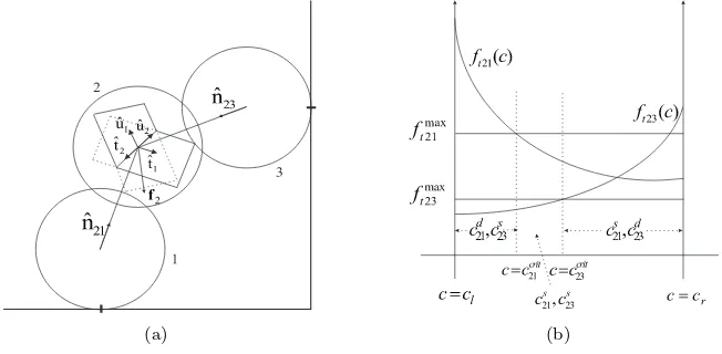
Before we try to deal with the complexity of multi-particle contacts, let us first consider a system in which a sphere is wedged into two fixed spheres, as shown in Fig. 1(a). The free sphere 2 has two contacts with the fixed spheres 1 and 3. Here we show that even for such a simple system, equation (1) can not fully describe the dynamics. The only moving sphere is sphere 2, the others are considered fixed, and we have three dimensional system. There are two contacts, so there are four unknowns and just three equations for zero acceleration of sphere 2 in the three directions. Apparently one degree of freedom is left, as we will show in more detail below. With rotation another three equations would be given by zero rotational acceleration of sphere 2, and we would not have the problem of indeterminacy, but rather too many constraints to be met.
(a) (b)
Figure 1: The collision geometry (a), and dependency of collision modes onc (b)
point, the related normal direction and tangential plane can always be identified. At each contact the colliding spheres exert a force onto each other with opposite direction. The force consists of a normal compression force, acting in the normal direction, e.g. nˆ21, and a tangential friction force, acting in the tangential plane spanned by ˆt1 and ˆt2. Suppose the line of intersection between the two tangent planes is in the direction of ˆu2, one of the unit vectors forming the tangent plane where sphere 2 collides with sphere 3, then we can establish a co-ordinate system consisting of the unit vectors ˆt1, ˆu1, and ˆu2 ( ˆt2 and ˆu2are collinear). Letft21and ft23 be the friction forces at the contact points of colliding sphere 2 with spheres 1 and 3 respectively. As derived in appendix A1, there is one free parameter, c. This parameter c can have any value in the range cl ≤ c ≤ cr, to give a static equation. In figure 1(b),ft21(c) and ft23(c) are the friction forces, andftmax21 and
fmax
t23 denote the maximum static friction forces at the related contact points. for which a transition to slipping occurs within the Coulomb model. These maximum forces determine the critical values of the free parameter.
If we choose the value of c in the interval ccrit
21 then the contact between spheres 1 and 2 is in the dynamic mode,cd
21, while the contact between spheres 2 and 3 is in the static mode,cs
23. Assigning a value ofcin the other intervals yields contact modes as shown in figure 1(b), where the superscript “s” and “d” stand for “static” and “dynamic”. Between the critical values there is a regime where both contacts can remain static. When the static contact mode is being maintained, the tangential force is evaluated using equations (9). On the other hand, when the colliding spheres start sliding the tangential force is given by the dynamic friction of equation (1).
Depending on the value ofc, figure 1(b) gives a tool to classify the contact modes and hence the tangential forces. Unfortunately, this value can not be deter-mined directly from the state variables. Thus, it is clearly shown that the Coulomb law can induces force indeterminacy in dynamic simulations where a sphere has two or more simultaneous collisions in three dimensions, as well as indeterminacy as to where a stick-slip transition will occur if stability is compromised.
2.2 Force models
2.2.1 Tangential force
To avoid the difficulties of Coulomb friction, fully dynamical models, where the static mode is approximated with little or no motion. Elperin and Golshtein [8] and Matuttiset al[13] introduce a tangential virtual spring once two spheres collide at timet0, as is pioneered by Cundall and Strack [6]. The model is represented by
ft=
½
−ˆδtkt|δt| ifkt|δt| ≤µ|fn|,
−ˆδtµ|fn| otherwise,
(2)
where ktdenotes the tangential spring constant, δt=
R
t0vt(τ)dτ is the total
The first term within the bracket in equation (2) represents the spring force during the “static” mode. The relative velocity may not be zero, but if the spring constant is sufficiently large, the tangential displacement will be small. When the force exceeds the threshold, given by the constraint, the spheres start sliding, and the friction force is given by the second term opposing the tangential displacement. Thus, there is a transition criterion from static to dynamic mode. This model gives a good agreement with experimental data for acetate spheres [15]. However, further investigations show that this model may lead to unphysical behaviour in the tangential force [8, 4] since in the model the friction force opposes the tangential displacement rather than the relative tangential velocity. Another shortcoming of this model is that it does not allow for a transition back from the dynamic to the static mode. Finally in the static mode the system may oscillate forever.
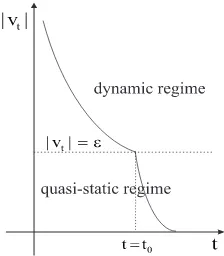
Figure 2: The transition of motion (schematic)
Elperin and Golshtein [8] and Brendel and Dippel [4] have made various suggestions to remedy the shortcomings mentioned. We have developed a model that includes a dynamic and a (quasi) static mode, and transitions between these, to describe the deposition process. In the static regime we use a (virtual) harmonic spring, as in the Cundall and Strack model, but with a damping term included. Furthermore, rather than engaging static mode at contact, an “ε - criterion” as shown in figure 2 is introduced: once the magnitude of relative tangential velocity is less than ε, the static regime engages, otherwise, the dynamic regime applies. When the spring force exceeds the Coulomb threshold, the spring is removed and the dynamic mode engages. During the quasi-static regime, the friction force is given by the damped spring, while beyond this regime the friction force is just proportional to the normal force. In addition, the model applies two different coefficients of friction,µsandµd . The tangential force is then modelled by
ft=
½
−(ktδt+γtvt), |vt| ≤ε(static mode)
−vtˆ µd|fn|, |vt|> ε(dynamic mode) (3)
the time when the quasi-static regime engages.
Oscillations in the static regime are avoided by applying critical damping,i.e.,
γt= 2
√
mkt. At the onset of the dynamic regime the velocity is small. To avoid the system engaging static mode again, we make the additional requirement that the tangential force opposes the velocity when applying the ε - criterium. As long as the velocity is increasing the dynamic mode will pertain. Hence the discontinuity at the transition from dynamic to static mode is replaced by a (short) transient.At the transition from static to dynamic the virtual spring is completely removed, all information about the direction or size on breaking is lost.
The simplicity of this model is that, unless theε - criterion is matched, it only applies dynamic friction, which is velocity independent. A similar velocity in-dependent model is also applied in [3, 17], but the virtual springs are implemented differently. Experimental results, using spherical glass particles [14] showed com-plicated behaviour of the stick - slip transition, with a continuously changing force, instead of a discrete step. It would be difficult to include these effects in the model.
2.2.1 Normal force
The second component of the contact force in our model is the compression force, perpendicular to the friction plane. In our model, it consists of an elastic and a dissipation force, modelled by a Hookean spring and damper
fn=−(knδn+γnvn), (4)
where δn and vn are the displacement (spheres may overlap) and the relative ve-locity in the normal direction, andkn and γn are the normal elastic and damping constants. The displacement is determined in practice by treating the grains as perfect spheres with a constant radius, and the displacement is simply the overlap between the (compressible) spheres. The tangential plane hence is always simply perpendicular to the vector connecting the centres of the colliding spheres. As the normal force, fn, is not constant, any quantities determined by the normal force, e.g., dynamic friction and maximum static friction, may vary over time, inducing transitions between static and dynamic modes.
The normal force (4) is simple in the sense that the elastic force is a linear function of the displacement, and the dissipation force is a linear function of the relative normal velocity. The simplicity leads to a non-zero force at the onset of contact due to the damping term [16, 12], which may not be appropriate. On the other hand, this simple model results in a coefficient of restitution, ψ, which is velocity independent. By applying the condition suggested by Luding [12], i.e., fn(tc) = 0, wheretcis the collision time,ψcan be related to the damping coefficient via
ψ=e−γnω(π−2 arctan(γnω)), withω=¡4mkt−γ2 n
¢
1 2
. (5)
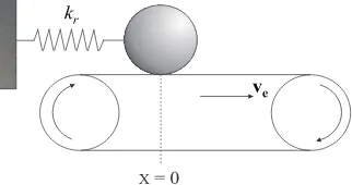
Figure 3: The conveyor belt
relates a model parameter, the normal damping coefficient, to an experimental system parameter, the coefficient of restitution.
2.3 A single sphere on the conveyor belt
To test our model with transitions between slip and stick motion we study a simple system of a single incompressible sphere on a conveyor belt. The sphere is connected to a fixed support by a spring having an elasticity constantkr, as shown in figure 3. The sphere is initially at rest with respect to the conveyor belt, and the spring is in the rest position. As the conveyor belt is driven with a constant velocityve, the sphere moves with the same velocity,vs=ve, causing the spring to stretch, generating the spring force,fsp=−kx. As long as the magnitude of spring force does not exceed the maximum static friction force,fmax
s , the sphere remains stationary with respect to the belt. We say the system is in the static mode. When the spring force exceeds the maximal static friction the sphere starts sliding along the belt, and the dynamic friction,fd, is applied. This we call the dynamic mode. When the relative velocity of the sphere drops below the critical value, the sphere re-sticks to the belt, and we have static mode again. The equation of motion of the sphere is then given by
½
˙
x=ve, |fsp| ≤fmax
s (static mode),
mx¨=fsp−fd, |fsp|> fmax
s (dynamic mode).
(6)
Equations (6) shows that during the static mode the sphere is displaced until
x = fmax
s /k. Furthermore, the dynamic mode always starts when x = fsmax/k and ˙x= ve, and the system returns to static mode when ˙x=ve or equivalently
x= (2µd−µs)mg. Hence, the system imposes the criteria to switch from static to dynamic modes and vice versa.
Since the relative velocity, vr = vs−ve, is always negative, the second equation of (6) can be rewritten in the form
½ x˙ =y
˙ y=−k
m(x−
|fd|
k ),
(7)
(|fd|/k,0), and its solution is given by
Substituting the first equation of (6) into equation (8) givesx1=µsmg/kand
x2= (2µd−µs)mg/k. Bothx1 and x2 denote the positions where the transitions occur. The first value is related to the transition from stick to slip, the second one is from slip to stick. The sphere undergoes a periodic stick-slip motion. In the phase plane, it is represented by a straight line during stick mode, and by a part of ellipse during the dynamic mode. Note the equation for x2 shows that if the roughness of the materials is such that µd ≤ 12µs then x2 ≤0, i.e. the spring is compressed prior to the transition.
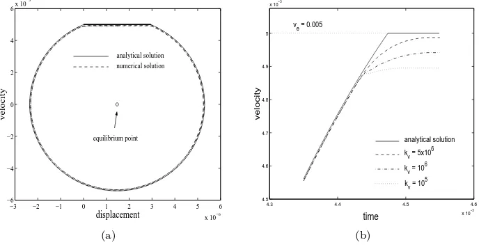
We want a numerical procedure to solve equation (6) to replicate this, es-pecially we want to avoid oscillatory behaviour near the transition from slip to stick. As a test, we apply our model of tangential friction (3) that introduces a virtual spring once the quasi-static regime is valid. In the first leg of the curve, the stick regime, we apply the Coulomb law. When the spring force exceeds the maximal static friction force, we use our model with the onset of the dynamic mode. The used parameters were a mass m = 0.05 kg, the gravitational acceler-ation g = 9.81 ms−2, stiffness of the real spring k
Figure 4: Phase plane of sphere’s motion (a) and vel. at stick-slip transition (b)
of error of the algorithm. The deviation occurs when the numerical procedure enters the quasi-static regime. When the dynamic friction disappears, the virtual spring and damping force build up the quasi-static regime. Initially these are less than the dynamic friction, so the velocity drops below the analytical curve. As can be seen from figure 4(b), the sphere actually never catches up with the belt. The reason is that in the static equilibrium the real spring force and the virtual spring force balance. The real spring force increases asfr
sp =−krx=krvet, so to match this the virtual spring force must befv
sp=kvδ=kvvvt, with vv=vekr/kv a remaining velocity difference between the belt and the sphere. The more rigid the virtual spring, the smaller the deviation from the analytical solution.
2.3 A small pile
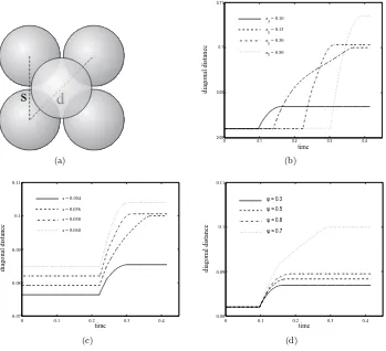
Figure 5: Five spheres construction (a) and behaviour of diagonal distance for varying initial height (b), init. mutual dist. of spheres (c), and coeff. of rest. (d)
square array of side lengths, and a fifth sphere is dropped from a vertical position exactly above the centre of the square, hitting the spheres on the floor. We use our model to investigate whether a stable pile structure results, with the upper sphere resting on the slightly extended array of four.
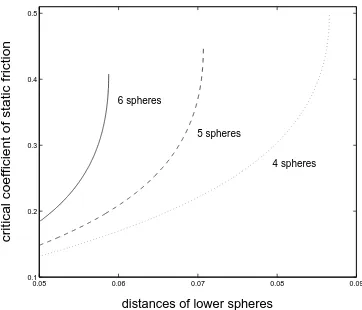
In appendix A2 we have investigated under what conditions this system allows a stable static pile structure. Figure 8 shows the critical static friction coefficient for a system consisting of 4, 5 and 6 spheres, as a function of the distance between the lower spheres. If the actual static friction coefficient is less than critical, the pile is unstable. Here we assumed the upper sphere is placed gently on the lower spheres. Dropping it from a distance has a destabilising effect.
We apply our quasi-static model once theε- criterion is satisfied. Throughout these simulations the used parameters values were diameter σ = 0.05 m, mass
m = 0.05 kg, elasticity constants in the normal and tangential directions kn =
kt = 105 kgs−2, friction coefficients µs = 0.6 and µd = 0.3, stick velocity ε = 10−3 ms−1, and time step is chosen sufficiently smaller than the smallest time scale occuring within our model system. We have varied the initial positions of the spheres (upper and lower spheres) and the normal damping constant (or the coefficient of restitution via equation (5)). In the simulations we only varied a single parameter, as a reference we used a normal damping constantγn= 0.5γncritor the coefficient of restitutionψ ≈0.3, whereγcrit
n is the normal critical damping. The diagonal distances of the lower spheres are shown in figures 5(b)–(d).
As shown in figures 5(b)–(d), when the upper sphere hits the lower spheres, they move apart. Depending on the applied parameters, the final diagonal distances may be less than twice the sphere diameter, in which case a stable pile is observed. If they exceed this value all spheres are on the surface. Figure 5(b) describes the effect of varying the initial vertical position of the upper sphere, z5. In this case the initial mutual distance of the lower spheres is 0.058 m. It can be seen that the higherz5, the flatter the pile structure. Atz5= 0.3 m there is no stable pile formed. For this value ofz5 a pile is formed if the initial gap is smaller,e.g. s= 0.054 m, as shown in figure 5(c) (initial height of the upper sphere = 0.3 m). Figure 5(d) (initial height of upper sphere = 0.1 m, and mutual distance of lower spheres = 0.058 m) shows the effect of the coefficient of restitutionψ. In figure 5(b), it can be seen that the system withs= 0.058 m,z5= 0.1 m andψ≈0.3 forms a stable pile. However, the same system withψ≈0.7 produces an unstable pile. As can be seen from figure 5(d), the upper sphere bounces back and hits the lower spheres again until they give way. In order for a larger pile of many particles to be stable, it is not completely necessary that the small system is stable. Once a somewhat dense layer of particles on the surface has formed, a particle on top of the layer must displace more than just the particle it is touching, and the friction forces involved may allow the formation of a larger pile.
2.3 Hourglass simulations
is obtained, the small pile simulation tells us what system parameters we must choose to obtain a stable pile. This first actual application of the model involves a system where particles fall one by one, from a certain vertical position, and with a small random horizontal velocity, onto a surface which has the same material properties as the objects. We have named these calculations hourglass simulations, as it mimics the free falling grains from the opening in an hourglass. The small horizontal velocity is needed to introduce some randomness in the system, and to avoid having all grains stack exactly on top of each other.
We simulate two and three dimensional (2D and 3D) systems consisting of 600 identical discs and 1200 spheres respectively. The parameter values were chosen similar to the previous problem,i.e.,σ= 0.05 m,m= 0.05 kg,kn=kt= 105kgs−2,
µs= 0.6,µd = 0.3,γn= 0.5γncrit,γt=γtcrit, and ε= 10−3 ms−1. Two time scales can be derived from the force equations 3 and 4. The oscillations of a particle of mass m in the normal direction with a force described by 4 occur on a time scale ofp
m/kn, which is 7×10⁻⁴ s for our values, provided the normal friction constant is small enough (γn ≤
√
mkn). For larger values of the dissipation in the normal direction the motion is critically or overdamped, leading to longer, rather than smaller time scales. As the dissipation in the tangential direction is critically damped, γt= 2
√
mkt, the time scale for the tangential force is
p
m/kt,
or 3.5×10⁻⁴ s. The time scale in the transition from dynamic to static mode is related to the critical velocity at which the transition occurs. Combination with the dynamic friction force yields a time scale ofmε/(µd|fn|), which may be interpreted as the time over which the velocity drops to zero given the force. The problem with this time scale is that it depends on the current value of the force. For the previous applications this time scale is not important, as the normal force is at about the order of the weight of a single grain. For real deposition with a large number of grains the normal force can be large. For a friction force of 10 kgms−2we obtain a time scale of 5×10⁻⁵ s. We set the time step to ∆t= 10−5 s.
(a) (b)
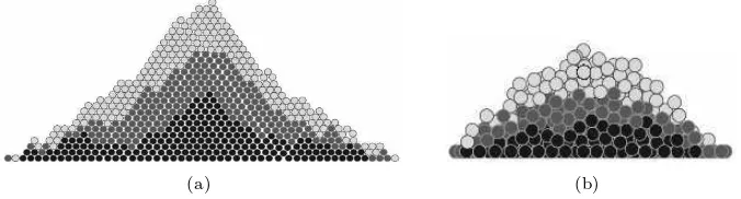
Figure 6: Stable piles of 600 discs (a), and 1200 spheres (b)
The pile almost forms a triangle with an irregular surface. Furthermore, it has an almost regular close packing structure with dislocation lines. In the dynamical study it was found that along these dislocation lines landslides occur, during which a large part of the pile shifts horizontally. 3D piles must have a much larger number of particles before a substantial pile, suited for analysis, is formed. To shorten the simulation time, grains are dropped in small batches of five. On the other aspects the model and procedure are analogous to the 2D case. Figure 6(b) shows the front view of the half part of the 3D pile cut by plane y = 0. The pile formed has a somewhat conical shape with spheres dropped earlier covered by the ones dropped later. Unlike the 2D pile, the structure of 3D pile, both inside and at the surface, is rather irregular.
3. CONCLUDING REMARKS
It has been shown that via a virtual spring with damping our friction model is able to describe the phenomena during the contact; from stick to slip, during slipping, and from slip to stick. The model solves the inherent problem of the Coulomb friction law, and has not shown any systematic error. As is shown in the phase plane of the conveyor belt problem, the model produces the same behaviour as the analytical solution, with slight deviation. Furthermore, the hourglass simu-lations show the model capable of generating stable piles, convincing it adequately captures this aspect of the deposition problem for which it was developed. In its present form the model may be used to study deposition of model materials or pile formations for which rolling is not important, if such materials do exist.
REFERENCES
1. J.J. Alonso and H.J. Herrmann, ”Shape of the tail of a two-dimensional sandpile”, Phys. Rev. Lett. 26 (76)(1996), 4911–4914.
2. P. Bak, C. Tang, and K. Wiesenfeld, ”Self-organised critically”,Phys. Rev. A,1
(38)(1988), 364-373.
3. J. Baxter, U. Tuzun, J. Burnell, and D.M. Heyes, ”Granular dynamics
simula-tions of two-dimensional heap formation”,Phys. Rev. E3 (55)(1997), 3546–3554.
4. L. Brendel and S. Dippel, ”Lasting contacts in molecular dynamics simulations”, in it Physics of dry granular materials, edited by H.J. Herrmann, J.P. Hovi and S. Luding, Kluwer, Dordrecht, 1998, 313–318.
5. V. Buchholtz and T. Poschel, ”Numerical investigation of the evolution of
sand-piles”,Physica A,202(1994), 390–401.
6. P.A. Cundall and O.D.L.Strack, ”A discrete numerical model for granular
assem-blies”,Geotechnique1 (29)(1979), 47–65.
8. T. Elperin and E. Golshtein, ”Comparison of different models for tangential forces
using the particle dynamics method”,Physica A,242(1997), 332–340.
9. Y. Grasselli, H.J. Herrmann, G. Oron, and S. Zapperi, ”Effect of impact energy
on the shape of granular heaps”,Granular Matter2(2000), 97–100.
10. Y. Grasselli and H.J. Herrmann, ”Crater formation on a three dimensional
gran-ular heap”,Granular Matter3(2001), 201–204.
11. G.A. Held, D.H. Solina, D.T. Keane, W.J. Haag, P.M. Horn, and G. Grin-stein, ”Experimental study of a critical-mass fluctuations in an evolving sandpile”, Phys. Rev. Lett. 9 (65)(1990), 1120–1123.
12. S. Luding, ”Collisions and contacts between two particles”, inPhysics of dry granular materials, edited by H.J. Herrmann,et al, Dordrecht, 1998, 285–303.
13. H.G. Matuttis, S. Luding, and H.J. Herrmann, ”Discrete element simulations
of dense packings and heaps made of spherical and non-spherical particles”, Powder
technology109(2000), 278–292.
14. S. Nasuno, A. Kudrolli, A. Bak and J.P. Gollub, ”Time-resolved studies of
stick-slip friction in sheared granular layers”,Phys. Rev. E,2 (58)(1998), 2161–2171.
15. J. Schafer, S. Dippel, and D.E. Wolf, ”Force schemes in simulations of granular
materials”,J. Phys. I France6(1996), 5–20.
16. D. Zhang and W.J. Whiten, ”The calculation of contact forces between particles
using spring and damping models”,Powder Technology,88(1996), 59–64.
17. Y.C. Zhou, B.D. Wright, R.Y. Yang, B.H. Xu, and A.B. Yu, ”Rolling friction in
the dynamic simulation of sandpile formation”,Physica A,269(1999), 536-553.
APPENDIX
A1. Friction force of two simultaneous contacts
At equilibrium, the Coulomb friction law of colliding bodies implies that the magnitude of the friction force is inside the friction cone. The actual value of this force balances the other forces acting on the body. We show in detail that direct implementation of the Coulomb friction leads to the problem of indeterminacy when there are too many contacts in the system.
Let us consider a system of a single sphere with two contact points, as is illustrated by figure 1. Here, sphere 2 has two simultaneous contacts with the fixed spheres 1 and 3. In equilibrium, the force balance in sphere 2 results in three equations and two relations with four unknowns. To calculate the friction force at each contact point on sphere 2 we work in a co-ordinate system consisting of the unit vectors ˆt1, ˆu1, ˆt2 and ˆu2, where ˆt2 and ˆu2 are taken along the intersection line of the tangential planes. Let ft21 andft23 be the friction forces at the contact points between spheres 2 and 1, and between spheres 2 and 3 respectively, then we have
where a1 andb1 are the coefficient of the vectors in the directions of ˆt1, and ˆu1, anda2 andb2 are the coefficients in the direction of ˆu2.
Letf2 be the sum of the force acting on sphere 2 due to gravity and com-pression. We want to investigate whether static equilibrium, implying that the resultant force of f2, ft21, and ft23 is zero, can be maintained. The force balance equation for sphere 2 is given by
f2=−¡a1ˆt1+b1uˆ1+ (a2+b2)ˆu2¢. (10)
The left side of equation (10) can be decomposed intof2k, acting in the plane spanned by ˆt1 and ˆu1, andf2⊥, acting in the intersection line and perpendicular to that plane, ˆu2. Hence, we have
f2k=−(a1ˆt1+b1ˆu1), and f2⊥=−(a2+b2)ˆu2. (11)
The left equation of (11) has a unique solution, while the right one has many solutions. Letb2=canda2=−(c+d). The equations in (9) can then be rewritten as
ft21=a1ˆt1−(c+d)ˆu2, and ft23=b1uˆ1+cuˆ2. (12)
Since for a given external force a1, b1, and d are fixed, but c is not, the friction forces depend on the chosen value of c. Let ft21(c) andft23(c) represent their magnitudes, they are then given by
ft21(c) =¡a21+ (c+d)2
t21 and ftmax23 be the maximum static friction forces at the related contact points. Let ccrit
21 and ccrit23 be the value ofc of each contacts when the magnitude of friction force equals to the maximum static friction. These (critical) values ofc
are then given by
A2. The critical coefficient of static friction
We investigate the possibility of having a stable pile when a sphere is placed on the top of several spheres at rest on a surface. All spheres are identical, and the surface has the same material properties as the spheres. The spheres can only slide, they do not roll.
Beginning with 4 spheres problem, we determine the critical coefficient of static friction,µc
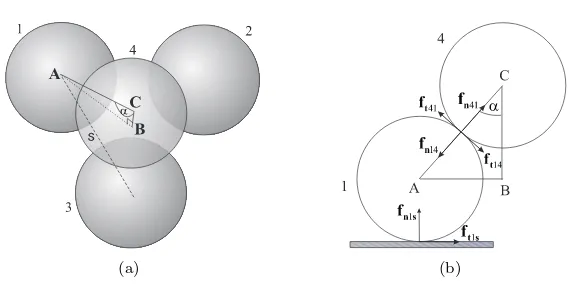
(a) (b)
Figure 7: The geometry of 4 spheres problem (a) and the symmetry plane used in the analysis with triangle ABC (b)
between sphere 1 and the surface. Figure 7(b) shows the section of intended plane. Triangle ABC connects the centres of spheres 1 and 4 (A and C), and the median of the equilateral triangle (B). Hence, the length of sides AC and AB are σ and
s/(2 sin(π/3)) respectively, whereσandsare the sphere diameter and the mutual distance between the lower spheres.
Letfn14 andft14 denote magnitude of the normal and tangential force com-ponents acting on sphere 1 due to the contact with sphere 4. Letfn1sand ft1s be the components of the contact force between sphere 1 and the surface. In this case
|fn1s|= 4mg/3. The force balance for sphere 1 is thus given by
|ft1s|+|ft14|cosα− |fn14|sinα= 0, (15)
|ft14|sinα+|fn14|cosα=mg
3 . (16)
The force balance for sphere 4 gives the same expression as equation(16). Clearly the problem results in two equations with three unknowns. Since our prob-lem is to determineµc
s, the least value ofµsfor which the system remains stable, the conditions|ft1s|=µs|fn1s|and|ft14|=µs|fn14|must be imposed. These equations together with equations (15) and (16) provide four equations with four unknowns, namely|ft1s|, |ft14|,|fn14|, andµs.
In term ofµs, one can obtain the quadratic equation
4 tanαµ2
s+ 5µs−tanα= 0. (17)
The critical coefficient of static friction,µc
s, is the relevant solution of equation (17), and is given by
µc s=
1 2
q
1 + 4(√54tanα)2−1 4
5tanα
In general for the n-spheres problem, equation (17) can be written in the form
ntanαµ2s+ (n+ 1)µs−tanα= 0. (19)
Hence,µc
sfor the n-spheres problem has the form
µc s=
1 2
q
1 + 4(n√+1n tanα)2−1 n
n+1tanα
, n= 4,5,6. (20)
In the above equations, as a function ofs,
tanα= p s/(2 sinβ)
σ2−(s/(2 sinβ))2, (21)
whereβ =π/(n−1), andsvalids in the intervalσ≤s <2σsinβ.
In figure 8 we have plotted the critical static friction coefficient for the 4, 5 and 6 sphere array, as a function of the distance between the centres of the lower spheres,s, rather than the angleα. The diameter of the spheres is,σ= 0.05 m, as in all our model calculations. If for a given coefficient of static frictionµc
sthe value of syields a point to the left of the corresponding curve, the pile is stable, but if that point is to the right of the curve, the pile is unstable.
0.05 0.06 0.07 0.08 0.09 0.1
0.2 0.3 0.4 0.5
distances of lower spheres
critical coefficient of static friction
6 spheres
5 spheres
4 spheres
Figure 8: Behaviour of the critical coefficient of static friction
M. Hasan: Department of Mathematics, Universitas Jember, Jember 68121, Indonesia. E-mail: [email protected].