Tweet sentiment analysis with classi
fi
er ensembles
Nádia F.F. da Silva
a,⁎
, Eduardo R. Hruschka
a, Estevam R. Hruschka Jr.
b aInstitute of Mathematics and Computer Sciences, University of São Paulo (USP), São Carlos, SP, BrazilbDepartment of Computer Science, Federal University of Sao Carlos (UFSCAR), São Carlos, SP, Brazil
a b s t r a c t
a r t i c l e
i n f o
Article history: Received 2 January 2014
Received in revised form 2 May 2014 Accepted 6 July 2014
Available online 24 July 2014
Keywords: Twitter Sentiment analysis Classifier ensembles
Twitter is a microblogging site in which users can post updates (tweets) to friends (followers). It has become an immense dataset of the so-calledsentiments. In this paper, we introduce an approach that automatically classifies the sentiment of tweets by using classifier ensembles and lexicons. Tweets are classified as either positive or negative concerning a query term. This approach is useful for consumers who can use sentiment analysis to search for products, for companies that aim at monitoring the public sentiment of their brands, and for many other applications. Indeed, sentiment classification in microblogging services (e.g., Twitter) through classifier ensembles and lexicons has not been well explored in the literature. Our experiments on a variety of public tweet sentiment datasets show that classifier ensembles formed by Multinomial Naive Bayes, SVM, Random Forest, and Logistic Regression can improve classification accuracy.
© 2014 Elsevier B.V. All rights reserved.
1. Introduction
Twitter is a popular microblogging service in which users post status messages, called“tweets”, with no more than 140 characters. In most cases, its users enter their messages with much fewer characters than the limit established. Twitter represents one of the largest and most dynamic datasets of user generated content—approximately 200 million users post 400 million tweets per day[1]. Tweets can express opinions on differ-ent topics, which can help to direct marketing campaigns so as to share consumers' opinions concerning brands and products[2], outbreaks of bul-lying[3], events that generate insecurity[4], polarity prediction in political and sports discussions[6], and acceptance or rejection of politicians[5], all in an electronic word-of-mouth way. Automatic tools can help decision makers to ensure efficient solutions to the problems raised. Under this per-spective, the focus of our work is on the sentiment analysis of tweets.
Sentiment analysis aims at determining opinions, emotions, and at-titudes reported in source materials like documents, short texts, sentences from reviews[7–9], blogs[10,11], and news[12], among other sources. In such application domains, one deals with large text corpora and most often“formal language”. At least two specific issues should be addressed in any type of computer-based tweet analysis:
first, the frequency of misspellings and slang in tweets is much higher than that in other domains, as users usually post messages from many different electronic devices, such as cell phones and tablets, and develop their own culture of a specific vocabulary in this type of environment.
Second, Twitter users post messages on a variety of topics, unlike blogs, news, and other sites, which are tailored to specific topics.
We consider sentiment analysis a classification problem. Just like in large documents, sentiments of tweets can be expressed in different ways and clas-sified according to the existence of sentiment, i.e., if there is sentiment in the message, then it is considered polar (categorized as positive or negative), otherwise it is considered neutral. Some authors, on the other hand, consider the six“universal”emotions[13]: anger, disgust, fear, happiness, sadness, and surprise as sentiments. In this paper, we adopt the view that sentiments can be either positive or negative, as in[14–18].
Big challenges can be faced in tweet sentiment analysis (Hassan et al. [19]): (i) neutral tweets are way more common than positive and neg-ative ones. This is different from other sentiment analysis domains (e.g. product reviews), which tend to be predominantly positive or negative; (ii) there are linguistic representational challenges, like those that arise from feature engineering issues; and (iii) tweets are very short and often show limited sentiment cues.
Many researchers have focused on the use of traditional classifiers, like Naive Bayes, Maximum Entropy, and Support Vector Machines to solve such problems. In this paper, we show that the use of ensembles of multiple base classifiers, combined with scores obtained from lexi-cons, can improve the accuracy of tweet sentiment classification. More-over, we investigate different representations of tweets that take bag-of-words and feature hashing into account[20].
The combination of multiple classifiers to generate a single classifier has been an active area of research over the last two decades[21–23]. For example, an analytical framework that quantifies the improvements in classification results due to the combination of multiple models is ad-dressed in[24]. More recently, a survey on traditional ensemble tech-niques—together with their applications to many difficult real-world problems, such as remote sensing, person recognition, and medicine— ⁎ Corresponding author at: Rua José Coelho Borgesn. 1235 Bairro Ipanema Sao Carlos, SP
Brazil -75705160. Tel:. +550416481354442.
E-mail addresses:[email protected](N.F.F. da Silva),[email protected](E.R. Hruschka), [email protected](E.R. Hruschka).
http://dx.doi.org/10.1016/j.dss.2014.07.003 0167-9236/© 2014 Elsevier B.V. All rights reserved.
Contents lists available atScienceDirect
Decision Support Systems
is presented in[24]. Studies on ensemble learning for sentiment analysis of large text corpora—like those found in movies and product reviews, web forum datasets, and question answering—are reported in[25–31]. In summary, the literature on the subject has shown that from indepen-dent, diversified classifiers, the ensemble created is usually more accu-rate than its individual components. Related work on tweet sentiment analysis is rather limited [32–34,19], but the initial results are promising.
Our main contributions can be summarized as follows: (i) we show that classifier ensembles formed by diversified components are promis-ing for tweet sentiment analysis; (ii) we compare bag-of-words and fea-ture hashing-based strategies for the representation of tweets and show their advantages and drawbacks; and (iii) classifier ensembles obtained from the combination of lexicons, bag-of-words, emoticons, and feature hashing are studied and discussed.
The remainder of the paper is organized as follows:Section 2 ad-dresses the related work.Section 3describes our approach, for which experimental results are provided inSection 4.Section 5concludes the paper and discusses directions for future work.
2. Related work
Several studies on the use of stand-alone classifiers for tweet senti-ment analysis are available in the literature, as shown in the summary
inTable 1. Some of them propose the use of emoticons and hashtags for building the training set, as Go et al.[35]and Davidov et al.[36], who iden-tified tweet polarity by using emoticons as class labels. Others use the characteristics of the social network as networked data, like in Hu et al. [37]. According to the authors, emotional contagion theories are material-ized based on a mathematical optimization formulation for the super-vised learning process. Approaches that integrate opinion mining lexicon-based techniques and learning-based techniques have been stud-ied. For example, Agarwal et al.[38], Read[39], Zhang et al.[40], and Saif et al.[41]used lexicons, part-of-speech, and writing style as linguistic resources. In a similar context, Saif et al.[42]introduced an approach to add semantics to the training set as an additional feature. For each extract-ed entity (e.g., iPhone), they addextract-ed its respective semantic concept (like “Apple's product”) as an additional feature and measured the correlation of the representative concept as negative/positive sentiments.
Classifier ensembles for tweet sentiment analysis have been underexplored in the literature—few exceptions are[32–34,19]. Lin and Kolcz[32]used Logistic Regression classifiers learned from 4-gram hashed byte as features.1They made no attempt to perform any
Table 1
Studies in tweet sentiment analysis.
Classification with lexicons and standalone learning algorithms
Study Year Feature set Lexicon Classifier Dataset
Read[39] 2005 N-gram Emoticons Naive Bayes and SVM Read[39]
Go et al. [35]
2009 N-gram and POS – Naive Bayes, Maximum
Entropy, and SVM
Go et al.[35]
Davidov et al. [36]
2010 Punctuation, n-grams, patterns, and tweet-based features – KNN O'Connor et al.[45]
Zhang et al. [40]
2011 N-gram, emoticons and hashtags Ding et al.[46] SVM Zhang et al.[40]
Agarwal et al. [38]
2011 POS, Lexicon, percentage of capitalized text, exclamation, capitalized text
Emoticons listed from Wikipediaa, an acronym dictionaryb
SVM Agarwal et al.[38]
Speriosu et al. [47]
2011 N-gram, hashtags, emoticons, lexicon and Twitter follower graph
Wilson et al.[48] Maximum Entropy Go et al.[35]and Speriosu et al.[47]
Saif et al. [42]
2012 N-gram, POS and semantic features – Naive Bayes Go et al.[35], Speriosu et al.[47] and Shamma et al. [49]
Hu et al. [37]
2013 N-gram, POS, data representation of social relations – – Go et al.[35]and Shamma et al.[49] Saif et al.
[41]
2013 N-gram, capitalized text, POS, lexicons Mohammad and Yang[50], Wilson et al. [48], Hu and Liu[9], and other lexicons constructed from hashtags
SVM Nakov et al.[51]
Ensemble learning
Study Year Feature set Base learner Ensemble methods Dataset
Lin and Kolcz [32]
2012 Feature hashing Logistic Regression classifier Majority vote Private dataset([32])
Rodriguez et al. [34]
2013 N-gram, lexicon, POS, tweet-based features and SentiWordnet
CRF, SVM and heuristic method Majority vote, upper bound, ensemble vote
Nakov et al.[51]
Clark et al. [33]
2013 N-gram, lexicon and polarity strength Naive Bayes Weighted voting scheme Nakov et al.[51]
Hassan et al. [19]
2013 A combination of unigrams and bigrams of simple words, part-of-speech and semantic features derived from WordNet[43]and SentiWordNet 3.0[44]
RBF Neural Network, RandomTree, REP Tree, Naive Bayes, Bayes Net, Logistic Re-gression and SVM.
linguistic processing, not even word tokenization. For each of the (pro-prietary) datasets, they experimented with ensembles of different sizes, composed of different models, and obtained from different training sets, however with the same learning algorithm (Logistic Regression). Their results show that the ensembles lead to more accurate classifiers. The authors also proposed an approach to obtain diversified classifiers by using different training datasets (over the random shuffle of the training examples)[32].Rodriguez et al.[34]and Clark et al.[33]proposed the use of classifier ensembles at expression-level, which is related to
Contextual Polarity Disambiguation. In this perspective, the sentiment label (positive, negative, or neutral) is applied to a specific phrase or word within the tweet and does not necessarily match the sentiment of the entire tweet. Finally, a promising ensemble framework was re-cently proposed by Hassan et al.[19], who deal with class imbalance, sparsity, and representational issues. The authors propose enriching the corpus by using multiple additional datasets also related to senti-ment classification. The authors use a combination of unigrams and bigrams of simple words, part-of-speech, and semantic features derived from WordNet[43]and SentiWordNet 3.0[44]. Also, they employed summarizing techniques, like Legomena and Named Entity Recognition. In our approach, we make use of feature hashing, which is a relative-ly new topic for text classification (broadly defined)—e.g., see[20, 52–54]. Note that in traditional document classification tasks, the input to the machine learning algorithm is a free text, from which a bag-of-words representation is constructed—the individual tokens are extracted, counted, and stored as vectors. Typically, in tweets, these vectors are extremely sparse. One can deal with this sparsity by using feature hashing. It is a fast way of building a vector space model of features, which turns features into either a vector or a matrix. Such an approach produces features represented as hash integers rather than strings. Asiaee et al.[55]showed that the performance of the classification can be improved in a low dimensional space via feature hashing[20]. Similarly, Lin and Kolcz[32]used feature hashing to deal with the high dimensional input space of tweets and showed that it can improve the performance of the machine learning algorithms.
We shall remark that our work differs from the existing work due to several aspects: (i) we compare bag-of-words and feature hashing based strategies for the representation of tweets and show their advan-tages and drawbacks; (ii) we study classifier ensembles obtained from the combination of lexicons, bag-of-words, emoticons, and feature hashing. Although Lin and Kolcz[32]used feature hashing in an ensem-ble of classifiers, they trained the classifiers in partitions of a private dataset and did not use lexicons and emoticons. They used only Logistic Regression as a classifier. Rodriguez et al.[34]and Clark et al.[33] pro-posed the use of classifier ensembles at expression-level, while we are interested in the use of classifier ensembles at tweet-level. Hassan
et al.[19]used a specific combination of datasets as training data, differ-ent features, differdiffer-ent classifiers, and different combination rules of clas-sifiers. We are interested in exposing the pros and cons of classifier ensembles in combination with two possibilities for the representation of a tweet—feature hashing and bag-of-words. We also explore the gains of the enrichment of the representations with lexicons.
3. Classifier ensembles for tweet sentiment analysis
Ensemble methods train multiple learners to solve the same prob-lem[22]. In contrast to classic learning approaches, which construct one learner from the training data, ensemble methods construct a set of learners and combine them. Dietterich[56]lists three reasons for using an ensemble based system:
Statistical Assume that we have a number of different
classi-fiers, and that all of them provide good accuracy in the training set. If a single classifier is chosen from the available ones, it may not yield the best generali-zation performance in unseen data. By combining the outputs of a set of classifiers, the risk of selecting an inadequate one is lower[21];
Computational Many learning algorithms work by carrying out a local search that may get stuck in local optima which may be far from global optima. For example, decision tree algorithms employ a greedy splitting rule and neural network algorithms employ gradient descent to minimize an error function over the train-ing set. An ensemble constructed by runntrain-ing the local search from many different starting points may provide a better approximation than any of the individual classifiers;
Representational If the chosen model cannot properly represent the sought decision boundary, classifier ensembles with diversified models can represent the decision bound-ary. Certain problems are too difficult for a given clas-sifier to solve. Sometimes, the decision boundary that separates data from different classes may be too com-plex and an appropriate combination of classifiers can make it possible to cope with this issue.
From a practical point of view, one may ask: What is the most appro-priate classifier for a given classification problem? This question can be interpreted in two different ways[22]: (i) What type of classifier should be chosen among many competing models, such as Support Vector Ma-chines (SVM), Decision Trees, Naive Bayes Classifier?; (ii) Given a par-ticular classification algorithm, which realization of this algorithm should be chosen? For example, different types of kernels used in SVM
can lead to different decision boundaries, even if all the other parame-ters are kept constant. Using an ensemble of such models and combin-ing their outputs — e.g. by averaging them — the risk of an unfortunate selection of a particularly poorly performing classifier can be reduced.
It is important to emphasize that there is no guarantee that the com-bination of multiple classifiers will always perform better than the best individual classifier in the ensemble. Except for certain special cases[57], the ensemble average performance can not be guaranteed. Combining classifiers may not necessarily beat the performance of the best classifier in the ensemble, however it certainly reduces the overall risk of making a poor selection of the classifier to be used with new (tar-get) data.
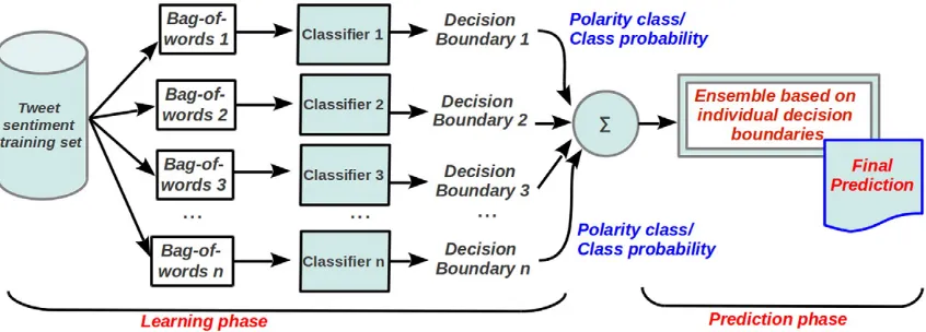
Effective ensembles require that the individual components exhibit some level of diversity[58,59,21,60]. Within the classification context, classifiers should generate different decision boundaries. If proper di-versity is achieved, independent errors are produced by each classifier, and combining them usually reduces the total error.Fig. 1, adapted from[61], illustrates this concept for a common setting in our particular application domain: each classifier, trained in a different subset of the available training data, produces different errors. However, the combi-nation of classifiers can provide the best decision boundary. Indeed, the Bayes error may be estimated from classifier ensembles[62]. Figs. 2 and 3provide examples of combination rules.
Brown et al.[63]suggested three methods for creating diversity in classifier ensembles: (i) varying the starting points within the hypothe-sis space (for example, by different initializations of the learning algo-rithm); (ii) varying the training set for the base classifiers; and (iii) varying the base classifiers or ensemble strategies. Our focus is on (iii), different from Lin and Kolcz[32]and Clark et al.[33]that addressed di-versity according to (ii), and Rodriguez et al.[34]that focus on an ex-pression-level analysis, applying diversity according to the training set for the base classifiers.
3.1. Our approach
Our hypothesis is that, by holding the philosophy underlying the use of classifier ensembles, endowed with appropriate feature engineering, accurate tweet sentiment classification can be obtained.
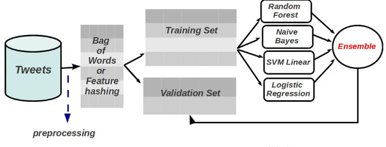
Fig. 4shows an overview of the approach adopted. Our base
classi-fiers are Random Forest, Support Vector Machines (SVM), Multinomial Naive Bayes, and Logistic Regression. Although we could have chosen other classifiers, the ones adopted here have been widely used in prac-tice, therefore they are suitable as a proof of concept.
In practice, classifiers are built to classify unseen data, usually re-ferred to as a target dataset. In a controlled experimental setting, as in the one addressed inSection 4, a validation set represents the target set. Actually, in controlled experimental settings the target set is fre-quently referred to as either a test or a validation set. These two terms have been used interchangeably, sometimes causing confusion. In our study, we assume that the target/validation set has not been used at all in the process of building the classifier ensembles. Once the base clas-sifiers have been trained, a classifier ensemble is formed by (i) the
average of the class probabilities obtained by each classifier or (ii) the majority voting.
The techniques used for feature representation (bag-of-wordsand
feature hashing) and preprocessing tweet data are addressed in details in the next subsections.
3.1.1. Feature representation
Two techniques for feature representation are particularly suitable for tweet sentiment classification:
• Bag-of-words. Tweets are represented by a table in which the columns represent the terms (or existing words) in the tweets and the values represent their frequencies. Therefore, a collection of tweets—after the preprocessing step addressed later—can be represented as illus-trated inTable 2, in which there aren tweetsandmterms.2Each tweet is represented astweeti= (ai1,ai2,…,aim), whereaijis the
fre-quency of termtjin thetweeti. This value can be calculated in various
ways.
• Feature hashing. It is used for text classification in[52,20,54,64,65]. For tweet classification, feature hashing offers an approach that re-duces the number of features provided as input to a learning algo-rithm. The original high-dimensional space is“reduced”byhashing
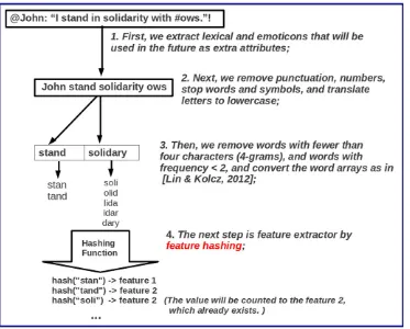
the features into a lower-dimensional space, i.e., mapping features to hash keys. Multiple features can be mapped to the same hash key, therefore their counts are“aggregated”.Fig. 5shows the application of feature hashing to the tweet“@John:“I stand in solidarity with
#ows.”!”. In the fourth step we use the hashing function in Eq.(1), which takes anl-length stringsas a parameter and returns the sum of ASCII values of their characters (ci).
h sð Þ ¼ΣliASCII cð Þ=10:i ð1Þ
3.1.2. Preprocessing
Retweets, stop words, links, URLs, mentions, punctuation, and ac-centuation were removed so that data set could be standardized. Stem-ming was performed so as to minimize sparsity. The bag-of-words was constructed with binary frequency, and a term is considered“frequent” if it occurs in more than one tweet.
We also used the opinion lexicon3proposed by Hu and Liu[9], who created a list of 4783 negative words and 2006 positive words. This list was compiled over many years and each of its words indicates an opin-ion. Positive opinion words are used to express desired states while neg-ative opinion words are used to express undesired states. Examples of positive opinion words arebeautiful,wonderful,good, andamazingand examples of negative opinion words arebad,poor, andterrible.
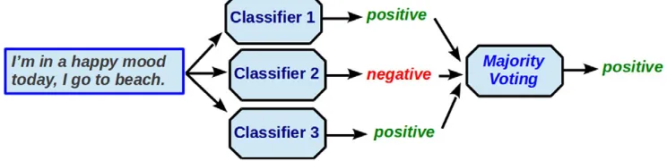
Fig. 2.An example of majority voting as the combination rule. In this case, the majority of the classifiers agree that the class is positive.
Emoticons available in the tweets have been used to enrich our fea-ture set. The number of positive and negative emotions was used to complement the information provided by the bag-of-words and the fea-ture hashing. Moreover, we computed the number of positive and neg-ative lexicons in each message.
4. Experimental evaluation
4.1. Datasets
Our experiments were performed in representative datasets obtain-ed from tweets on different subjects[66]:
4.1.1. Sanders—Twitter Sentiment Corpus
It consists of hand-classified tweets collected from four Twitter search terms: @apple, #google, #microsoft, and #twitter. Each tweet has a sentiment label: positive, neutral, negative, and irrelevant. As in [67], we reported only the classification results for positive and negative classes, which resulted in 570 positive and 654 negative tweets.
4.1.2. Stanford—Twitter Sentiment Corpus
This dataset[35]has 1,600,000 training tweets collected by a scraper that queries the Twitter API. The scraper, periodically, sends a query to the positive emotion–:)–and a separate query to the negative emotion–:(–at the same time. After removing retweets, any tweet containing both positive and negative emoticons, repeated tweets, and bias caused by the emotions, one gets 800,000 tweets with positive emoticons and 800,000 tweets with negative emoticons. In contrast to the training set, which was collected based on specific emoticons, the test set was collected by searching Twitter API with specific queries and including product names, companies, and people. The tweets were manually annotated with a class label and 177 negative and 182 positive tweets were obtained. Although the Stanford test set is relative-ly small, it has been widerelative-ly used in the literature in different evaluation tasks. For example, Go et al.[35], Saif et al.[42], Speriosu et al.[47], and
Bakliwal et al.[68]use it to evaluate their models for polarity classifi ca-tion (positive vs. negative). In addica-tion to polarity classification, Marquez et al.[69]use this dataset for evaluating subjectivity classifi ca-tion (neutral vs. polar).
4.1.3. Obama-McCain Debate (OMD)
This dataset was constructed from 3238 tweets crawled during the
first U.S. presidential TV debate that took place in September 2008 [49]. The sentiment ratings of the tweets were acquired by using the Amazon Mechanical Turkte4. Each tweet was rated as positive, negative, mixed, and others.“Other”tweets are those that could not be rated. We kept only the tweets rated by at least three voters, which comprised a set of 1906 tweets, from which 710 were positive and 1196 were nega-tive ones. In another configuration of the dataset, we considered only tweets with unanimity of opinion. We named it Strict Obama-McCain Debate (OMD) dataset, which has 916 tweets—347 positive and 569 negative.
4.1.4. Health care reform (HCR)
This dataset was built by crawling tweets containing the hashtag “#hcr”(health care reform) in March 2010[47]. A subset of this corpus was manually annotated as positive, negative, and neutral. The neutral tweets were not considered in the experiments, thus the training dataset contained 621 tweets (215 positive and 406 negative) whereas the test set contained 665 (154 positive and 511 negative).
4.2. Experimental setup
We conducted experiments in the WEKA platform5to run Multino-mial Naive Bayes, Logistic Regression, and Random Forests. We used the Library for Support Vector Machines[70]LibSVM6for training SVM
4 https://www.mturk.com/.
5 http://www.cs.waikato.ac.nz/ml/weka/. 6 http://www.csie.ntu.edu.tw/cjlin/libsvm/.
Fig. 4.Overview of our approach.
Fig. 3.An example of averaging probabilities as the combination rule. In this case, probability P(class = positive tweet)NP(class = negative tweet), then the output of the ensemble is positive.
classifiers. ForObama-McCainDebate andSanders Twitter Sentiment
datasets we used the standard 10-fold cross validation. ForHealth Care Reformdataset, we used the same training and test folds available in the public resource[42]. Finally, for theStanford Twitter Sentiment Corpuswe did samplings from the original training set and validated in the test set available in[35].
4.3. Results
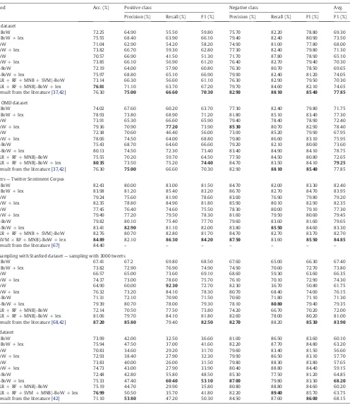
We compared the results of stand-alone classifiers with those of our ensemble approach described inSection 3.1. By considering different combinations of bag-of-words (BoW), feature hashing (FH), and lexi-cons, we can evaluate the potential of ensembles to boost classification accuracy. The best results described in the literature are also reported for comparison purposes.
Table 3shows the results of the BoW-based approaches, whereas Table 4focuses on the results of feature hashing. According to the ta-bles, our ensembles provided accuracy gains in all assessed settings. As expected, the use of classifier ensembles may lead to additional computational costs, however accuracy gains are usually worth-while. In pairwise comparisons of classifiers with and without lexicons, the former ones provided better results in all the
experiments. As mentioned inSection 3.1, the lexicon dictionary was constructed for reviews of products sold on-line[9]. It consists of informal words, as well as types of messages, found in tweets. In the Stanford dataset the improvement was more relevant since the data has been collected from emoticons. In this type of dataset, there is no specific domain, while the other datasets address more specific topics, like technology (Sanders), politics (Strict OMD and OMD) and health (HCR dataset).
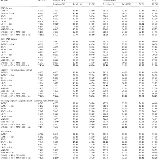
According to the feature hashing results (Table 4), our ensembles showed better accuracy rates than single base classifiers for all the datasets. By taking the average of the positive and negative F-Measure into account, we obtained the best results in 80% of the BoW cases. Note that feature hashing provides worse results than BoW in most of the datasets, except for the HCR dataset, where the results have shown to be the best in literature—including here our own results for the BoW-based ensemble. However, as expected, feature hashing enables a significant reduction in dimensionality, as shown inTable 5, and there is a trade-off between classification accuracy and computational savings. It is important to reinforce that none of the results reported in the literature make use of any di-mensionality reduction technique and thereby can not be compared to our results obtained with feature hashing. To the best of our knowledge, feature hashing has not been assessed in public data sets for the sentiment analysis of tweets.
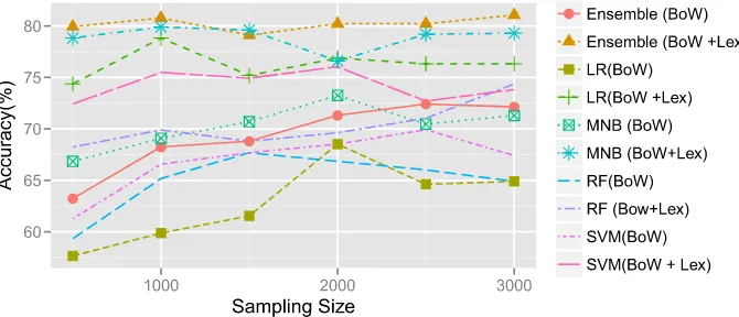
Some additional experiments for the Stanford dataset were also con-ducted. Due to computational limitations, we did not run experiments with the complete training data, but from balanced random sampling, whose sample sizes varied from 500 to 3000 tweets. We chose stand-alone classifiers as baselines to be compared to our ensemble approach. By considering different combinations of bag-of-words (BoW) and lex-icons, we can evaluate the potential of ensembles to boost classification accuracy.Fig. 6shows the overall picture of all machine learning
Table 2
Representation of tweets.
t1 t2 … tm
tweet1 a11 a12 … a1m
tweet2 a21 a22 … a2m
… … … … …
tweetn an1 an2 … anm
algorithms used. Note that the ensemble obtained from BoW and lexi-cons has provided the best results. More importantly and in contrast to the other approaches, very good classification accuracy rates were obtained even for small sample sizes. The best accuracy rate reported in the literature for the complete dataset (formed by 1,600,000 tweets)
is 87.20%, whereas our ensemble trained with only 0.03% of the data ob-tained an accuracy of 81.06% in the test set available in[35].
Finally, it is worth comparing our results to those obtained in[19]. However, the datasets used in that study are not publicly available, ex-cept for Sanders. For this data, we carried out experiments considering
Table 3
Cross comparison results for bag-of-words (best results in bold). LR, RF, and MNB refer to Logistic Regression, Random Forest, and Multinomial Naive Bayes, respectively. ENS indicates the use of ensembles, BoW refers to bag-of-words, lex refers to lexicon, and the SVM-BoW + lex abbreviation indicates that we used SVM with bag-of-words and lexicon as features. Other abbreviations are Acc. for the accuracy, F1 for the F-measure, and Avg for the average of positive and negative F-measures.
Method Acc. (%) Positive class Negative class Avg.
Precision (%) Recall (%) F1 (%) Precision (%) Recall (%) F1 (%) F1 (%)
OMD dataset
SVM-BoW 72.25 64.90 55.50 59.80 75.70 82.20 78.80 69.30
SVM-BoW + lex 75.55 68.40 63.90 66.10 79.40 82.40 80.90 73.50
RF-BoW 71.04 62.90 54.20 58.20 74.90 81.00 77.80 68.00
RF-BoW + lex 73.82 66.70 59.30 62.80 77.30 82.40 79.80 71.30
LR-BoW 70.57 66.90 41.50 51.30 71.70 87.80 78.90 65.10
LR-BoW + lex 73.85 66.10 56.90 61.20 76.40 82.70 79.40 70.30
MNB-BoW 72.19 64.00 57.90 60.80 76.30 80.70 78.50 69.65
MNB-BoW + lex 75.97 68.80 65.10 66.90 79.90 82.40 81.20 74.05
ENS(LR + RF + MNB + SVM)-BoW 73.14 66.30 56.60 61.10 76.30 82.90 79.50 70.30 ENS(LR + RF + MNB)-BoW + lex 76.81 71.10 63.70 67.20 79.70 84.60 82.10 74.65 Best result from the literature[37,42] 76.30 75.00 66.60 70.30 82.90 88.10 85.40 77.85
Strict OMD dataset
SVM-BoW 74.02 67.60 60.20 63.70 77.30 82.40 79.80 71.75
SVM-BoW + lex 78.93 73.80 68.90 71.20 81.80 85.10 83.40 77.30
RF-BoW 73.91 65.30 66.60 65.90 79.40 78.40 78.90 72.40
RF-BoW + lex 79.36 70.90 77.20 73.90 85.30 80.70 82.90 78.40
LR-BoW 72.38 70.60 46.40 56.00 73.00 85.20 79.90 67.95
LR-BoW + lex 78.06 74.50 64.00 68.80 79.80 86.60 83.10 75.95
MNB-BoW 75.43 68.70 64.60 66.60 79.20 82.10 80.60 73.60
MNB-BoW + lex 80.13 74.50 72.30 73.40 83.40 84.90 84.10 78.75
ENS(LR + RF + MNB)-BoW 75.55 70.20 59.70 64.50 77.50 84.50 80.80 72.65
ENS(LR + RF + MNB)-BoW + lex 80.35 73.50 75.20 74.40 84.70 83.50 84.10 79.25
Best result from the literature[37,42] 76.30 75.00 66.60 70.30 82.90 88.10 85.40 77.85
Sanders—Twitter Sentiment Corpus
SVM-BoW 82.43 80.00 83.00 81.50 84.70 82.00 83.30 82.40
SVM-BoW + lex 83.98 81.20 85.40 83.20 86.70 82.70 84.70 83.95
RF-BoW 79.24 75.60 81.90 78.60 83.00 76.90 79.80 79.20
RF-BoW + lex 82.35 78.80 84.90 81.80 85.90 80.10 82.90 82.35
LR-BoW 77.45 76.40 74.60 75.50 78.30 80.00 79.10 77.30
LR-BoW + lex 79.49 77.20 79.50 78.30 81.60 79.50 80.60 79.45
MNB-BoW 79.82 80.10 75.40 77.70 79.60 83.60 81.60 79.65
MNB-BoW + lex 83.41 82.90 81.10 82.00 83.80 85.50 84.60 83.30
ENS(LR + RF + MNB + SVM)-BoW 82.76 80.70 82.80 81.70 84.70 82.70 83.70 82.70 ENS(SVM + RF + MNB)-BoW + lex 84.89 82.10 86.30 84.20 87.50 83.60 85.50 84.85
Best result from the literature[67] 84.40 – – – – – – –
Best sampling with Stanford dataset—sampling with 3000 tweets
SVM-BoW 67.41 67.2 69.80 68.50 67.60 65.00 66.30 67.40
SVM-BoW + lex 73.82 72.90 76.90 74.90 74.90 70.60 72.70 73.80
RF-BoW 66.57 65.00 73.60 69.10 68.60 59.30 63.60 66.35
RF-BoW + lex 74.37 73.00 78.60 75.70 76.10 70.10 72.90 74.30
LR-BoW 64.90 60.00 92.30 72.70 82.30 36.70 50.80 61.75
LR-BoW + lex 76.32 73.20 84.10 78.30 80.70 68.40 74.00 76.15
MNB-BoW 71.31 72.10 70.90 71.50 70.60 71.80 71.10 71.30
MNB-BoW + lex 79.39 80.70 78.00 79.30 78.10 80.80 79.40 79.35
ENS(LR + RF + MNB)-BoW 72.14 70.50 77.50 73.80 74.20 66.70 70.20 72.00
ENS(LR + RF + MNB)-BoW + lex 81.06 79.70 84.10 81.80 82.60 78.00 80.20 81.00 Best result from the literature[68,42] 87.20 85.80 79.40 82.50 82.70 88.20 85.30 83.90
HCR dataset
SVM-BoW 73.99 42.00 32.50 36.60 81.00 86.50 83.60 60.10
SVM-BoW + lex 75.94 47.50 37.00 41.60 82.20 87.70 84.80 63.20
RF-BoW 70.83 34.60 29.20 31.70 79.60 83.40 81.50 56.60
RF-BoW + lex 72.93 38.40 27.90 32.30 79.90 86.50 83.10 57.70
LR-BoW 73.83 40.00 26.00 31.50 79.80 88.30 83.80 57.65
LR-BoW + lex 74.73 43.00 27.90 33.90 80.40 88.80 84.40 59.15
MNB-BoW 72.48 42.80 55.80 48.50 85.30 77.50 81.20 64.85
MNB-BoW + lex 75.33 47.40 60.40 53.10 87.00 79.80 83.30 68.20
ENS(LR + RF + MNB)-BoW 75.19 44.70 29.90 35.80 80.80 88.80 84.60 60.20
ENS(LR + RF + SVM + MNB)-BoW + lex 76.99 50.50 35.70 41.80 82.20 89.40 85.70 63.75 Best result from the literature[42] 71.10 53.80 47.20 50.30 84.50 87.60 86.00 68.15
the neutral class7and 10-fold cross validation. We assume that a neutral lexicon exists when neither positive nor negative lexicon exist in the opinion lexicon (Hu and Liu[9]). We obtained an accuracy rate of 76.25%, while Hassan et al.[19]obtained 76.30%. Our results are very good in comparison to theirs, since they used more linguistic resources and classifier models, and also expanded the number of patterns by in-cluding instances from different sub-domains.
Table 4
Cross comparison results using feature hashing (FH)—best results in bold.
Method Acc. (%) Positive class Negative class Avg.
Precision (%) Recall (%) F1 (%) Precision (%) Recall (%) F1 (%) F1 (%)
OMD dataset
SVM-FH 51.10 37.90 49.20 42.80 63.40 52.30 57.30 50.05
SVM-FH + lex 62.85 50.10 57.60 53.60 72.40 66.00 69.00 61.30
RF-FH 61.39 47.10 29.60 36.30 65.80 80.30 72.30 54.30
RF-FH + lex 67.37 58.50 42.50 49.30 70.60 82.10 75.90 62.60
LR-FH 63.28 61.90 3.70 6.90 63.30 98.70 77.10 42.00
LR-FH + lex 70.57 67.00 41.30 51.10 71.60 88.00 78.90 65.00
MNB-FH 62.54 47.20 4.80 8.70 63.10 96.80 76.40 42.55
MNB-FH + lex 70.41 64.40 45.90 53.60 72.60 84.90 78.30 65.95
ENS(LR + RF + MNB)-FH 64.59 39.80 32.00 35.50 63.80 71.30 67.40 51.45
ENS(LR + RF + MNB)-FH + lex 70.62 57.70 53.70 55.60 73.60 76.70 75.10 65.35
Strict OMD dataset
SVM-FH 51.31 39.80 55.30 46.30 64.20 48.90 55.50 50.90
SVM-FH + lex 62.99 51.30 47.00 49.00 69.20 72.80 71.00 60.00
RF-FH 61.36 48.50 31.70 38.30 65.60 79.40 71.90 55.10
RF-FH + lex 72.60 69.00 50.10 58.10 73.90 86.30 79.60 68.85
LR-FH 65.29 65.30 17.90 28.10 65.30 94.20 77.10 52.60
LR-FH + lex 73.03 68.10 54.20 60.40 75.20 84.50 79.60 70.00
MNB-FH 60.70 36.20 4.90 8.60 62.00 94.70 75.00 41.80
MNB-FH + lex 71.39 66.20 50.10 57.00 73.50 84.40 78.60 67.80
ENS(LR + RF + MNB)-FH 65.17 59.60 23.30 33.50 65.90 90.30 76.20 54.85
ENS(LR + RF + MNB)-FH + lex 74.56 70.20 57.10 63.00 76.50 85.20 80.60 71.80
Sanders–Twitter Sentiment Corpus
SVM-FH 49.75 46.30 49.80 48.00 53.20 49.70 51.40 49.70
SVM-FH + lex 75.00 74.10 71.20 72.60 75.70 78.30 77.00 74.80
RF-FH 55.64 52.10 59.80 55.70 59.80 52.00 55.60 55.65
RF-FH + lex 71.63 68.00 73.90 70.80 75.40 69.70 72.40 71.60
LR-FH 56.94 54.70 43.50 48.50 58.20 68.70 63.00 55.75
LR-FH + lex 75.98 74.40 73.90 74.10 77.40 77.80 77.60 75.85
MNB-FH 54.25 51.00 45.30 48.00 56.50 62.10 59.20 53.60
MNB-FH + lex 75.08 73.30 73.20 73.20 76.60 76.80 76.70 74.95
ENS(LR + RF + MNB)-FH 57.84 53.70 49.30 51.40 58.80 63.00 60.80 56.10
ENS(LR + RF + MNB)-FH + lex 76.63 75.40 73.20 74.30 77.20 79.20 78.20 76.25
Best sampling with Stanford dataset—sampling with 3000 tweets
SVM-FH 47.63 47.50 31.90 38.20 47.70 63.80 54.60 46.40
SVM-FH + lex 54.32 54.00 66.50 59.60 54.80 41.80 47.40 53.50
RF-FH 47.63 52.50 58.80 55.40 51.60 45.20 48.20 51.80
RF-FH + lex 70.47 70.40 72.00 71.20 70.50 68.90 69.70 70.45
LR-FH 55.71 56.20 57.10 56.70 55.20 54.20 54.70 55.70
LR-FH + lex 78.55 76.60 83.00 79.70 80.90 74.00 77.30 78.50
MNB-FH 54.32 54.50 59.30 56.80 54.00 49.20 51.50 54.15
MNB-FH + lex 78.27 77.40 80.80 79.00 79.30 75.70 77.50 78.25
ENS(LR + RF + MNB)-FH 57.38 55.30 54.40 54.80 53.90 54.80 54.30 54.55
ENS(LR + RF + MNB)-FH + lex 79.11 76.90 78.60 77.70 77.50 75.70 76.60 77.15
HCR dataset
SVM-FH 67.22 28.40 27.30 27.80 78.30 79.30 78.80 53.30
SVM-FH + lex 69.92 20.50 10.40 13.80 76.50 87.90 81.80 47.80
RF-FH 63.16 25.10 29.90 27.30 77.60 73.20 75.30 51.30
RF-FH + lex 72.48 38.70 45.50 41.80 82.60 78.30 80.40 61.10
LR-FH 67.52 26.90 23.40 25.00 77.80 80.80 79.30 52.15
LR-FH + lex 77.6 50 17.50 26.00 79.20 94.70 86.30 56.15
MNB-FH 73.83 34.80 10.40 16.00 77.70 94.10 85.10 50.55
MNB-FH + lex 75.34 46.50 26.00 33.30 80.30 91.00 85.30 59.30
ENB(LR + RF + MNB)-FH 76.09 27.50 7.10 11.30 77.10 94.30 84.90 48.10
ENB(LR + RF + MNB)-FH + lex 78.35 52.90 29.90 38.20 81.30 92.00 86.30 62.20
7Hassan et al.[19]use other datasets, however they are not available.
Table 5
Number of features from bag-of-words and from feature hashing.
Dataset # of features
from BoW
# of features from FH
OMD dataset 1352 13
Strict OMD dataset 759 10
Sanders—Twitter Sentiment Corpus 1203 23
Stanford dataset 2137 21
5. Concluding remarks
The use of classifier ensembles for tweet sentiment analysis has been underexplored in the literature. We have demonstrated that classifier ensembles formed by diversified components—specially if these come from different information sources, such as textual data, emoti-cons, and lexicons —can provide state-of-the-art results for this particular domain. We also compared promising strategies for the rep-resentation of tweets (i.e., bag-of-words and feature hashing) and showed their advantages and drawbacks. Feature hashing has shown to be a good choice in the scenario of tweet sentiment analysis where computational effort is of paramount importance. However, when the focus is on accuracy, the best choice is bag-of-words. Although our re-sults have been obtained for data from Twitter, one of the most popular social media platforms, we believe that our study is also relevant for other social media analyses.
As future work we are going to study neutral tweets[19], where datasets are enriched with analogue domain datasets, and with differ-ent features. As it is widely known, diversity is a key point for the suc-cessful application of ensembles. Therefore, more effort will be devoted towards this direction.
Acknowledgments
The authors would like to acknowledge Research Agencies CAPES (DS-7253238/D), FAPESP (2013/07787-6 and 2013/07375-0), and CNPq (303348/2013-5) for theirfinancial support. They are also grateful to Marko Grobelnik for pointing out some related work on tweet analysis.
References
[1] A. Ritter, S. Clark, Mausam, O. Etzioni, Named entity recognition in tweets: an exper-imental study, Proceedings of the Conference on Empirical Methods in Natural Lan-guage Processing, EMNLP'11, Association for Computational Linguistics, Stroudsburg, PA, USA, 2011, pp. 1524–1534.
[2] B.J. Jansen, M. Zhang, K. Sobel, A. Chowdury, Twitter power: Tweets as electronic word of mouth, Journal of the American Society for Information Science and Tech-nology 60 (11) (2009) 2169–2188.
[3] J.-M. Xu, K.-S. Jun, X. Zhu, A. Bellmore, Learning from bullying traces in social media, HLT-NAACL, , The Association for Computational Linguistics, 2012. 656–666. [4] M. Cheong, V.C. Lee, A microblogging-based approach to terrorism informatics:
ex-ploration and chronicling civilian sentiment and response to terrorism events via twitter, Information Systems Frontiers 13 (1) (2011) 45–59.
[5] P.H.C. Guerra, A. Veloso, W. Meira, V. Almeida Jr, From bias to opinion: a transfer-learning approach to real-time sentiment analysis, Proceedings of the 17th ACM SIGKDD Conference on Knowledge Discovery and Data Mining, San Diego, CA, 2011. [6] N.A. Diakopoulos, D.A. Shamma, Characterizing debate performance via aggregated twitter sentiment, Proceedings of the SIGCHI Conference on Human Factors in Com-puting Systems, CHI'10, ACM, New York, NY, USA, 2010, pp. 1195–1198. [7] P.D. Turney, Thumbs up or thumbs down?: semantic orientation applied to
unsu-pervised classification of reviews, Proceedings of the 40th Annual Meeting on
Association for Computational Linguistics, ACL 02, Association for Computational Linguistics, Stroudsburg, PA, USA, 2002, pp. 417–424.
[8] B. Pang, L. Lee, S. Vaithyanathan, Thumbs up? Sentiment classification using ma-chine learning techniques, Proceedings of EMNLP, 2002, pp. 79–86.
[9] M. Hu, B. Liu, Mining and summarizing customer reviews, Proceedings of the Tenth ACM SIGKDD International Conference on Knowledge Discovery and Data Mining, KDD'04, ACM, New York, NY, USA, 2004, pp. 168–177.
[10]B. He, C. Macdonald, J. He, I. Ounis, An effective statistical approach to blog post opinion retrieval, Proceedings of the 17th ACM Conference on Informa-tion and Knowledge Management, CIKM'08, ACM, New York, NY, USA, 2008, pp. 1063–1072.
[11] P. Melville, W. Gryc, R.D. Lawrence, Sentiment analysis of blogs by combining lexical knowledge with text classification, Proceedings of the 15th ACM SIGKDD Interna-tional Conference on Knowledge Discovery and Data Mining, KDD'09, ACM, New York, NY, USA, 2009. 1275–1284.
[12] A. Balahur, R. Steinberger, M. Kabadjov, V. Zavarella, E. van der Goot, M. Halkia, B. Pouliquen, J. Belyaeva, Sentiment analysis in the news, in: N. C. C. Chair), K. Choukri, B. Maegaard, J. Mariani, J. Odijk, S. Piperidis, M. Rosner, D. Tapias (Eds.), Proceedings of the Seventh International Conference on Language Re-sources and Evaluation (LREC'10), European Language ReRe-sources Association (ELRA), Valletta, Malta, 2010.
[13] P. Ekman, Emotion in the Human Face, vol. 2Cambridge University Press, 1982. [14]B. Liu, Sentiment analysis and opinion mining, Synthesis Lectures on Human
Lan-guage Technologies, Morgan & Claypool Publishers, 2012.
[15] B. Liu, Web data mining: exploring hyperlinks, contents, and usage data, Data-Centric Systems and Applications, Springer-Verlag New York, Inc., Secaucus, NJ, USA, 2006.
[16] B. Liu, Sentiment Analysis and Subjectivity, Taylor and Francis Group, Boca, 2010. [17] A. Agarwal, P. Bhattacharyya, Sentiment analysis: a new approach for effective use
of linguistic knowledge and exploiting similarities in a set of documents to be clas-sified, Proceedings of the International Conference on Natural Language Processing (ICON), 2005.
[18]S.S. Standifird, Reputation and e-commerce: ebay auctions and the asymmetrical impact of positive and negative ratings, Journal of Management 27 (3) (2001) 279–295.
[19]A. Hassan, A. Abbasi, D. Zeng, Twitter Sentiment Analysis: A Bootstrap Ensemble Framework, SocialCom, IEEE, 2013. 357–364.
[20]K.Q. Weinberger, A. Dasgupta, J. Langford, A.J. Smola, J. Attenberg, Feature hashing for large scale multitask learning, in: A.P. Danyluk, L. Bottou, M.L. Littman (Eds.), ICML, Vol. 382 of ACM International Conference Proceeding Series, ACM, 2009, p. 140.
[21] L.I. Kuncheva, Combining Pattern Classifiers: Methods and Algorithms, Wiley-Interscience, 2004.
[22] Z. Zhou, Ensemble methods: foundations and algorithms, Chapman & Hall/CRC Data Mining and Knowledge Discovery Series, Taylor & Francis, 2012.
[23]J.A. Benediktsson, J. Kittler, F. Roli, Multiple classifier systems, Vol. 5519 of Lecture Notes in Computer Science, Springer, Reykjavik, Iceland, 2009.
[24] K. Tumer, J. Ghosh, Analysis of decision boundaries in linearly combined neural clas-sifiers, Pattern Recognition 29 (1996) 341–348.
[25] G. Wang, J. Sun, J. Ma, K. Xu, J. Gu, Sentiment classification: the contribution of en-semble learning, Decision Support Systems (0) (2013).
[26]A. Abbasi, H. Chen, S. Thoms, T. Fu, Affect analysis of web forums and blogs using correlation ensembles, IEEE Transactions on Knowledge and Data Engineering 20 (9) (2008) 1168–1180.
[27] Heterogeneous ensemble learning for Chinese sentiment classification, Journal of In-formation and Computational Science 9 (15) (2012) 4551–4558.
[28] B. Lu, B. Tsou, Combining a large sentiment lexicon and machine learning for subjec-tivity classification, 2010 International Conference on Machine Learning and Cyber-netics (ICMLC), vol. 6, 2010, pp. 3311–3316.
[29] Y. Su, Y. Zhang, D. Ji, Y. Wang, H. Wu, Ensemble learning for sentiment classification, in: D. Ji, G. Xiao (Eds.), Chinese Lexical Semantics, Vol. 7717 of Lecture Notes in Com-puter ScienceSpringer, Berlin Heidelberg, 2013, pp. 84–93.
[30]M. Whitehead, L. Yaeger, Sentiment mining using ensemble classification models, in: T. Sobh (Ed.), Innovations and Advances in Computer Sciences and Engineering, Springer, Netherlands, 2010, pp. 509–514.
[31]A. Abbasi, H. Chen, S. Thoms, T. Fu, Affect analysis of web forums and blogs using correlation ensembles, IEEE Transactions on Knowledge and Data Engineering 20 (9) (2008) 1168–1180.
[32] J. Lin, A. Kolcz, Large-scale machine learning at twitter, Proceedings of the 2012 ACM SIGMOD International Conference on Management of Data, SIGMOD'12, ACM, New York, NY, USA, 2012, pp. 793–804.
[33] S. Clark, R. Wicentwoski, Swatcs: combining simple classifiers with estimated accu-racy, Second Joint Conference on Lexical and Computational Semantics (*SEM), Pro-ceedings of the Seventh International Workshop on Semantic Evaluation (SemEval 2013), vol. 2, Association for Computational Linguistics, Atlanta, Georgia, USA, 2013, pp. 425–429.
[34]C. Rodriguez Penagos, J. Atserias, J. Codina-Filba, D. Garcıa-Narbona, J. Grivolla, P. Lambert, R. Saur, Fbm: combining lexicon-based ml and heuristics for social media polarities, Proceedings of SemEval-2013—International Workshop on Semantic Evaluation Co-located with *Sem and NAACL, Atlanta, Georgia, 2013, (url date at 2013-10-10).
[35] A. Go, R. Bhayani, L. Huang, Twitter sentiment classification using distant supervi-sion,Unpublished Manuscript,Stanford University1–6.
[36] D. Davidov, O. Tsur, A. Rappoport, Enhanced sentiment learning using twitter hashtags and smileys, Proceedings of the 23rd International Conference on Compu-tational Linguistics: Posters, COLING'10, Association for CompuCompu-tational Linguistics, Stroudsburg, PA, USA, 2010, pp. 241–249.
[37]X. Hu, L. Tang, J. Tang, H. Liu, Exploiting social relations for sentiment analysis in microblogging, Proceedings of the Sixth ACM International Conference on Web Search and Data Mining, 2013.
[38] A. Agarwal, B. Xie, I. Vovsha, O. Rambow, R. Passonneau, Sentiment analysis of twit-ter data, Proceedings of the Workshop on Languages in Social Media, LSM'11, Asso-ciation for Computational Linguistics, Stroudsburg, PA, USA, 2011, pp. 30–38. [39] J. Read, Using emoticons to reduce dependency in machine learning techniques for
sentiment classification, Proceedings of the ACL Student Research Workshop, ACLstudent'05, Association for Computational Linguistics, Stroudsburg, PA, USA, 2005, pp. 43–48.
[40] L. Zhang, R. Ghosh, M. Dekhil, M. Hsu, B. Liu, Combining lexicon-based and learning-based methods for twitter sentiment analysis, HP Laboratories, 2011. (technical Report).
[41]S. Mohammad, S. Kiritchenko, X. Zhu, Nrc-Canada: building the state-of-the-art in sentiment analysis of tweets, Proceedings of the Seventh International Workshop on Semantic Evaluation Exercises (SemEval-2013), Atlanta, Georgia, USA, 2013. [42]H. Saif, Y. He, H. Alani, Semantic sentiment analysis of twitter, Proceedings of the
11th International Conference on The Semantic Web—Volume Part I, ISWC'12, Springer-Verlag, Berlin, Heidelberg, 2012, pp. 508–524.
[43] G.A. Miller, Wordnet: a lexical database for english, Communications of the ACM 38 (11) (1995) 39–41.
[44] S. Baccianella, A. Esuli, F. Sebastiani, Sentiwordnet 3.0: An enhanced lexical resource for sentiment analysis and opinion mining, in: N. C. C. Chair), K. Choukri, B. Maegaard, J. Mariani, J. Odijk, S. Piperidis, M. Rosner, D. Tapias (Eds.), Proceedings of the Seventh International Conference on Language Resources and Evaluation (LREC 10), European Language Resources Association (ELRA), Valletta, Malta, 2010. [45] B. O'Connor, R. Balasubramanyan, B.R. Routledge, N.A. Smith, From tweets to polls: linking text sentiment to public opinion time series, Proceedings of the International AAAI Conference on Weblogs and Social Media, 2010.
[46] X. Ding, B. Liu, P.S. Yu, A holistic lexicon-based approach to opinion mining, Proceed-ings of First ACM International Conference on Web Search and Data Mining (WSDM-2008), 2008.
[47] M. Speriosu, N. Sudan, S. Upadhyay, J. Baldridge, Twitter polarity classification with label propagation over lexical links and the follower graph, Proceedings of the First Workshop on Unsupervised Learning in NLP, EMNLP'11, Association for Computa-tional Linguistics, Stroudsburg, PA, USA, 2011, pp. 53–63.
[48]T. Wilson, J. Wiebe, P. Hoffmann, Recognizing contextual polarity in phrase-level sentiment analysis, Proceedings of the Conference on Human Language Technology and Empirical Methods in Natural Language Processing, HLT'05, Association for Computational Linguistics, Stroudsburg, PA, USA, 2005, pp. 347–354.
[49] D.A. Shamma, L. Kennedy, E.F. Churchill, Tweet the debates: understanding commu-nity annotation of uncollected sources, In WSM?09: Proceedings of the International Workshop on Workshop on Social, 2009.
[50]S.M. Mohammad, P.D. Turney, Emotions evoked by common words and phrases: using mechanical turk to create an emotion lexicon, Proceedings of the NAACL HLT 2010 Workshop on Computational Approaches to Analysis and Generation of Emotion in Text, CAAGET'10, Association for Computational Linguistics, Stroudsburg, PA, USA, 2010, pp. 26–34.
[51] P. Nakov, S. Rosenthal, Z. Kozareva, V. Stoyanov, A. Ritter, T. Wilson, Semeval-2013 task 2: sentiment analysis in twitter, Second Joint Conference on Lexical and Com-putational Semantics (*SEM), Proceedings of the Seventh International Workshop on Semantic Evaluation (SemEval 2013), vol. 2, Association for Computational Lin-guistics, Atlanta, Georgia, USA, 2013, pp. 312–320.
[52] Q. Shi, J. Petterson, G. Dror, J. Langford, A. Smola, S. Vishwanathan, Hash kernels for structured data, Journal of Machine Learning Research 10 (2009) 2615–2637. [53] K. Ganchev, M. Dredze, Small statistical models by random feature mixing,
Proceed-ings of the ACL-2008 Workshop on Mobile Language Processing, Association for Computational Linguistics, 2008.
[54] G. Forman, E. Kirshenbaum, Extremely fast text feature extraction for classification and indexing, CIKM'08: Proceeding of the 17th ACM Conference on Information and Knowledge Management, ACM, New York, NY, USA, 2008. 1221–1230. [55]A. Asiaee, T.M. Tepper, A. Banerjee, G. Sapiro, If you are happy and you know it…
tweet, Proceedings of the 21st ACM International Conference on Information and Knowledge Management, CIKM'12, ACM, New York, NY, USA, 2012, pp. 1602–1606. [56] T.G. Dietterich, Ensemble methods in machine learning, Proceedings of the First In-ternational Workshop on Multiple Classifier Systems, MCS'00, Springer-Verlag, London, UK, 2000, pp. 1–15.
[57]G. Fumera, F. Roli, A theoretical and experimental analysis of linear combiners for multiple classifier systems, IEEE Transactions on Pattern Analysis and Machine In-telligence 27 (6) (2005) 942–956.
[58]K. Tumer, J. Ghosh, Error correlation and error reduction in ensemble classifiers, Connection Science 8 (3–4) (1996) 385–403.
[59] A. Krogh, J. Vedelsby, Neural network ensembles, cross validation, and active learn-ing, Advances in Neural Information Processing Systems, , MIT Press, 1995. 231–238. [60] L.I. Kuncheva, C.J. Whitaker, Measures of diversity in classifier ensembles and their relationship with the ensemble accuracy, Machine Learning 51 (2) (2003) 181–207. [61] R. Polikar, Ensemble learning, Scholarpedia 4 (1) (2009) 2776.
[62] K. Tumer, J. Ghosh, Bayes error rate estimation using classifier ensembles, Interna-tional Journal of Smart Engineering System Design 5 (2) (2003) 95–110. [63] G. Brown, J. Wyatt, R. Harris, X. Yao, Diversity creation methods: a survey and
categorisation, Information Fusion 6 (2005) 5–20.
[64] J. Langford, A. Strehl, L. Li, Vowpal Wabbit online learning project,http://mloss.org/ software/view/53/2007.
[65] C. Caragea, A. Silvescu, P. Mitra, Protein Sequence Classification Using Feature Hashing, in: F.-X. Wu, M.J. Zaki, S. Morishita, Y. Pan, S. Wong, A. Christianson, X. Hu (Eds.), BIBM, IEEE, 2011, pp. 538–543.
[66] H. Saif, M. Fernandez, Y. He, H. Alani, Evaluation datasets for twitter sentiment anal-ysis: a survey and a new dataset, the STS-Gold, in: C. Battaglino, C. Bosco, E. Cambria, R. Damiano, V. Patti, P. Rosso (Eds.), ESSEM@AI*IA, Vol. 1096 of CEUR Workshop Proceedings, CEUR-WS.org, 2013, pp. 9–21.
[67] D. Ziegelmayer, R. Schrader, Sentiment polarity classification using statistical data compression models, in: J. Vreeken, C. Ling, M.J. Zaki, A. Siebes, J.X. Yu, B. Goethals, G.I. Webb, X. Wu (Eds.), ICDM Workshops, IEEE Computer Society, 2012, pp. 731–738.
[68] A. Bakliwal, P. Arora, S. Madhappan, N. Kapre, M. Singh, V. Varma, Mining senti-ments from tweets, Proceedings of the 3rd Workshop in Computational Approaches to Subjectivity and Sentiment Analysis, Association for Computational Linguistics, Jeju, Korea, 2012, pp. 11–18, (URLhttp://www.aclweb.org/anthology-new/W/ W12/W12-3704.bib).
[69] F. Bravo-Marquez, M. Mendoza, B. Poblete, Combining strengths, emotions and po-larities for boosting twitter sentiment analysis, Proceedings of the Second Interna-tional Workshop on Issues of Sentiment Discovery and Opinion Mining, WISDOM'13, ACM, New York, NY, USA, 2013, pp. 2:1–2:9.