Survivor interaction contrast wiggle pre

Contents lists available atScienceDirect

Journal of Mathematical Psychology

journal homepage:www.elsevier.com/locate/jmp

Survivor interaction contrast wiggle predictions of parallel and serial

models for an arbitrary number of processes

Haiyuan Yang

a,∗

_{, Mario Fific}

b

_{, James T. Townsend}

a a_{Department of Psychological and Brain Sciences, Indiana University, Bloomington, IN, 47405, USA} b_{Psychology Department, Grand Valley State University, MI, 49401, USA}

h i g h l i g h t s

• We explore the precise behavior of the serial exhaustive SIC function forn=2. • We provide a generalization of the SIC function to an arbitrary number of processes.

• We analyze the generalized SIC for both parallel and serial models with minimum and maximum time stopping rules. • We demonstrate application of the theorems to data from a short-term memory search task.

a r t i c l e i n f o

Article history:

Keywords:

Survivor interaction contrast Human information processing Logarithmic concavity Multi-processes

a b s t r a c t

The Survivor Interaction Contrast (SIC) is a distribution-free measure for assessing the fundamental prop-erties of human information processing such as architecture (i.e., serial or parallel) and stopping rule (i.e., minimum time or maximum time). Despite its demonstrated utility, there are some vital gaps in our knowledge: first, the shape of the serial maximum time SIC is theoretically unclear, although the one 0-crossing negative-to-positive signature has been found repeatedly in the simulations. Second, the the-ories of SIC have been restricted to two-process cases, which restrict the applications to a limited class of models and data sets. In this paper, we first prove that in the two-process case, a mild condition known as strictly log-concavity is sufficient as a guarantor of a single 0-crossing of the serial maximum time SIC. We then extend the definition of SIC to an arbitrary number of processes, and develop implicated methodol-ogy of SIC in its generalized form, again in a distribution-free manner, for both parallel and serial models in conjunction with both the minimum time and maximum time stopping rules. We conclude the paper by demonstrating application of the theorems to data from a short-term memory search task.

©2013 Published by Elsevier Inc.

1. Introduction

The question of whether people can perform multiple percep-tual or mental operations simultaneously, that is, parallel process-ing, vs. whether items or tasks must proceed serially (one at a time), has intrigued psychologists since the birth of experimen-tal psychology. Historically, reaction time (RT) has been the pri-mary measure on this question. The work of the physiologist F.C. Donders (e.g.,Donders, 1868) was seminal in this regard, although other researchers, such as W. Wundt, were more prolific with re-gard to early results on human cognition.

With the revolution brought about through cognitive science and cognitive psychology in the 1950s and 1960s, questions such as the parallel vs. serial conundrum, which had lain dormant since the nineteenth century saw a renaissance of interest.

∗Corresponding author.

E-mail addresses:haiyyang@indiana.edu(H. Yang),fificm@gvsu.edu(M. Fific), jtownsen@indiana.edu(J.T. Townsend).

The serial vs. parallel topic is our primary concern here. How-ever, it may be worth a moment’s pondering, given the pioneering role of William K. Estes in the advent of mathematical psychol-ogy, of how the latter field, and Estes’ research, fit into, and con-tributed to, modern cognitive psychology. Three tributaries fed the new stream of mathematical psychology in the 1950s and 60s. These were: 1. Signal detection theory, child of psychophysics and sensory processes, mathematical communications theory, applied physics, and statistical decision making (e.g.,Green & Swets, 1966; Tanner & Swets, 1954). 2. Foundational measurement the offspring of S.S. Stevens’ brilliant but non-rigorous statements concern-ing measurement in psychology fostered and rendered rigorous through strands from philosophy, mathematical logic and abstract algebra (e.g., Krantz, Luce, Suppes, & Tversky, 1971; Roberts & Zinnes, 1963). 3. Mathematical learning theory which went back at least to Clark Hull (e.g.,Hull, 1952); or see Koch’s elegant summary in Modern Learning Theory (Koch, 1954). This branch is where we find the Estes trailblazing Stimulus Sampling Theory (Estes,1955, 1959), a precise, quantitative theory of human and animal learning.

This theory, which still impacts a wide spectrum of research in cog-nition today, led to a score of research advances by Estes and col-leagues as well as a host of other scientists (e.g.,Atkinson & Estes, 1963;Friedman et al.,1964).

Estes was an early entrant into the embryonic cognitive move-ment. His research in this domain was likely influenced by the burgeoning efforts utilizing the information processing approach, perhaps the early dominant theme in this new domain. Early pio-neers included Wendell Garner (e.g.,Garner, 1962), Donald Broad-bent (e.g.,Broadbent, 1958), William Hick (e.g. Hick, 1952), and Colin Cherry (e.g.Cherry, 1953) (note the heavy presence of British psychologists).

American psychologists were soon contributing to this rapidly expanding field which bridged sensory processes, higher percep-tion, and elementary cognition. Prime examples are Charles Erik-sen (e.g.,Eriksen & Spencer, 1969), Michael Posner (e.g.,Posner, 1978), Raymond Nickerson (e.g.,Nickerson, 1972), Ralph Haber (e.g.,Haber & Hershenson, 1973), and Howard Egeth (e.g.,Egeth, 1966). And, Bill Estes of course.

The employment of ingenious experimental designs to answer questions concerning whether humans perform visual or mem-ory search in a serial or parallel fashion provide apt examples of new trends making an appearance in the 60s and 70s. (e.g., Sper-ling,1960,1967;Sternberg,1966,1975). Estes and colleagues pro-vided some classic early results in this domain in extending, and mathematically modeling extensions of Sperlings innovative visual search experimental designs. For instance,Estes and Taylor(1964) developed a new detection method as well as associated models in this vein. Also,Estes and Taylor(1966) andEstes and Wessel (1966) were beginning to explore phenomena and human informa-tion processing mechanisms related to the presence of redundant signals in visual displays.

TheSternberg(1966) innovative and rather startling RT data in short term memory search, in particular, had a profound influence on thinking in the parallel vs. serial processing literature. In fact, a massive body of experimental literature over several decades has been based on the inference that increasing, more-or-less straight-line RT functions of the workloadn,1_{the number of comparisons}

to perform, imply serial processing. However, the ability of lim-ited capacity parallel models to mimic serial models, in the strong sense of mathematical equivalence, was demonstrated relatively early on (e.g.,Atkinson, Holmgren, & Juola, 1969;Murdock,1971; Townsend,1969,1971).2_{And in fact, the reverse possibility of}

se-rial models to mimic parallel models was also proven (Townsend, 1969,1971,1972,1974). The early mathematical results were con-fined to limited types of RT distributions, but later developments extended to arbitrary probability distributions (Townsend,1976; Townsend & Ashby, 1983;Vorberg,1977).

The parallel models which perfectly mimic serial models are

limited capacityin the sense that their processes degrade in their

ef-ficiency as the workloadnincreases. Such models intuitively make the predictions associated with serial processing, specifically the linear RT graphs of the workloadn(e.g.,Townsend, 1971). Fortu-nately, theory-driven experimental methodologies have been in-vented in recent years that are considerably more robust in the

1 An increment in workload is usually natural to define in terms of number of dimensions, or subtasks involved in some task. We shall often refer simply to items or, sometimes, processes as generic tags for the discrete objects being processed or the conduits working on them. The unit of workload typically relates in a natural fashion to the task. For example, if a memory search task involves examination of a list of letters, the unit may be made straightforwardly in terms of letters. Thennmay stand for both the workload in the task and the number of letters in the memory set.

2 For an up to date review of the parallel–serial identifiability issue, see

Townsend, Yang, and Burns(2011).

assessment of mental architecture, particularly serial vs. parallel processing (Scharff, Palmer, & Moore, 2011;Townsend,1976,1981, 1990a;Townsend & Nozawa, 1995;Townsend & Wenger, 2004). In particular, the new methodologies often allow architectural infer-ences even though the workload is held constant, so that capacity does not confound architectural inferences.

Our focus here lies within the general approach referred to as

Systems Factorial Technology(hereafter SFT; seeTownsend,1992;

Townsend & Nozawa, 1995). A number of investigators have made essential contributions to this literature including Schweickert and Dzhafarov and colleagues (Dzhafarov, 1997; Dzhafarov, Schwe-ickert, & Sung, 2004; Schweickert, 1978, 1982; Schweickert & Giorgini, 1999;Schweickert, Giorgini, & Dzhafarov, 2000). SFT re-lies heavily on mathematical propositions indicating experimental conditions where strong tests of architectures may be found, al-though other testable features, such as capacity, are also encom-passed presently. The bulk of theoretical work has been performed under the assumption ofselective influence. Our scope prohibits de-tails here, but we can loosely define selective influence as the prop-erty that certain experimental factors act only on specific processes in the overall system (see Section2.1for more detailed discussion on selective influence). When selective influence is in force, pre-dictions of serial and parallel models and the pertinent decisional stopping rules are strikingly distinct. This paper is intended to sig-nificantly strengthen and extend these predictions.

SFT requires the survivor function S

(

t

)

, which is simply the complement of the well-known cumulative distribution (or fre-quency) function (the CDF) written asF

(

t

)

. That is,S

(

t

)

₌

1

₋

F

(

t

)

. A central statistical diagnostic is then the survivor interaction con-trast (or SIC) function. It performs a double difference concon-trast op-eration on the survivor functions that is analogous to the mean interaction contrast (or MIC) employed on the arithmetic RT means in earlier investigations (e.g.,Schweickert,1978;Sternberg,1966). However, it now expresses a highly diagnostic function of time, rather than a single number.

Despite the successful deployment of the SIC measure, there are some vital gaps in our knowledge, restricting the applications to a limited class of models and data sets. These will be sketched within a brief presentation of relevant knowledge we do have.

We know that, forn

₌

2, serial minimum time models predict perfectly flat signatures whereas serial maximum time (i.e., the classical exhaustive processing time stopping rule; seeSternberg, 1969;Townsend,1974) predictions must include at least one wig-gle (i.e., the up-and-down excursions marked by 0-crossings) be-low and above 0 (Townsend & Nozawa, 1995). However, although simulations have intimated that there is a single wiggle passing through 0, in a negative-to-positive direction as exhibited inFig. 1 (the top right panel), this has not been shown to be true for all dis-tributions. In fact, the exact shape of the SIC curve is as yet un-known.

Therefore, in elucidating further properties of serial exhaustive processing: A. We first prove that serial exhaustive processing in-evitably predicts an odd number of 0-crossings in then

₌

2 case. B. Next, we show that a certain readily-met mathematical condi-tion is sufficient to force the behavior indicated through our simu-lations, a single 0-crossing of the SIC function.

The behavior our SIC signatures have also remained unidenti-fied forn

>

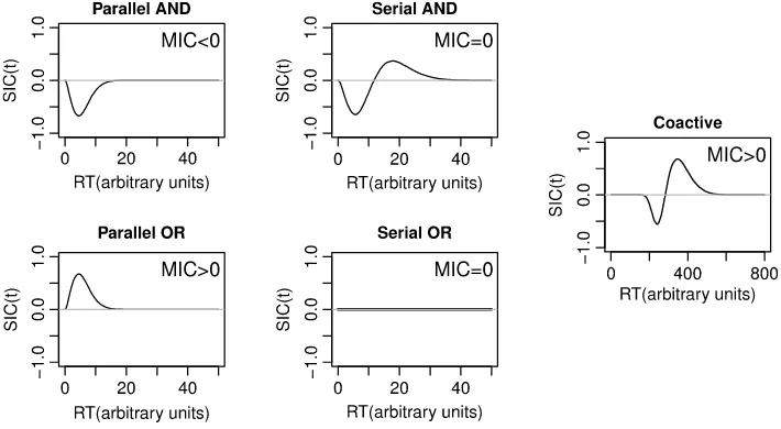
2, in the case of all studied serial and parallel processes up to now. The quite intriguing behaviors in the case of the serial and parallel models with varying stopping rules, and for arbitrary values ofn, are next developed for: A. Serial minimum time pro-cessing. B. Serial maximum time propro-cessing. C. Parallel minimum time processing. D. Parallel maximum time processing.

Fig. 1. Representative predictions of survivor interaction contrast (SIC) and mean interaction contrast (MIC) across different architectures and stopping rules. The four canonical models on the left are based on simulations of gamma distributions, with various shape parameters regarding different salience levels of processes. The coactive model on the right is based on simulations of dynamic systems described in (Townsend & Wenger, 2004).

Fig. 2. Distributional influences of the high vs. low salience manipulation with survivor functions (right) and densities suggesting satisfaction of the one point crossover (left). The simulations are based on gamma distributions with different shape parameters.

2. Extending knowledge of serial exhaustive processing: analy-sis for two processes

2.1. Underlying assumptions of SFT

The critical assumption underlying SFT is selective influence, which means that an experimental factor affects only a single pro-cess. We continued the convention (Townsend & Ashby, 1983) of indicating the level of a factor as high if it speeds up the process and as low when it slows down the process. Manipulating the speed of the process is also referred to as salience manipulation. In the short-term memory search task shown in the exemplar experi-ment section, for instance, high dissimilarity between the item in the memory and the target will be designated as a high salience level, and low dissimilarity between item and target will be desig-nated as a low salience level.

In terms of RT distribution, an experimental variable acting se-lectively could in principle affect any one or more of several aspects of an RT distribution. In this paper we follow the assumption as ex-pressed inTownsend and Nozawa(1995) that the two processing time density functions for a single process, at the two factor levels cross exactly once, i.e., there is exactly one timet∗_{, where the two}

density functions are equal. This assumption implies an ordering of both survivor functions (i.e. stochastic dominance) as well as the means and medians. This assumption appears to be satisfied within the limits of typical psychological applications (e.g.,Townsend,

1990b;Townsend & Nozawa, 1995).Fig. 2shows a hypothetical example of selective influence operating at the one-point density

crossover level, using two gamma distributed variables. We can see that the property of single density crossover (left panel) leads to both an ordering of the survivor functions (right panel) and of the mean processing times (right panel, the area under the survivor curves).

In order to avoid possible failure of selective influence due to in-direct non-selective influence, i.e., one factor can inin-directly affect the ‘wrong’ process through stochastic dependence (Townsend,

1984; Townsend & Thomas, 1994), some condition concerning stochastic independence is typically required. For simplicity of proof, stochastic independence of the process completion times is assumed, althoughDzhafarov (1999,2003)andDzhafarov et al.

(2004) has shown that conditional independence given some com-mon sources of randomness which are unaffected by the experi-mental factors is sufficient for these purposes.3

Therefore, not only must selective influence act at a level of suf-ficient power on a processX(e.g., the density single point crossing assumption above), but it must be assumed that the marginal prob-ability functions on processing times for all other processesY,Z, etc. must be invariant when theXfactor is manipulated. Base times (all else besides the completion times of the processes in which we are interested) are avoided in this study but under the assumption of conditional independence, would not affect our results in any event.

2.2. Limited review of systems factorial technology

Suppose we are concerned with just two processes or channels. We refer to these asXand Y. Letf_XL

(

t

)

be the density function of the processing time onXwhen the factor level of processXis low andfXH

(

t

)

be the density function of the processing time onX

when the factor level is high. Likewise, letf_YL

(

t

)

andf_YH

(

t

)

be the density functions of the processing time onYwhen the factor level ofYis low and high, respectively. In this paper we assume that all density functions are sufficiently smooth.4LetSXL

(

t

)

,SXH

(

t

)

,SYL

(

t

)

andSYH

(

t

)

denote the survivor functions corresponding tofXL

(

t

)

,

fXH

(

t

)

,fYL

(

t

)

andfYH

(

t

)

respectively. A survivor function of random

variableTis defined as

S

(

t

)

=

P

(

T

>

t

)

=



∞

t

f

(

t′

)

dt′

=

1

−

F

(

t

).

(1)

The Survivor Interaction Contrast (SIC) function of the total re-action timeT (later we useT with subscripts to denote reaction times of single process) is defined as

SIC2

(

t

)

=

(

SLL

(

t

)

−

SLH

(

t

))

−

(

SHL

(

t

)

−

SHH

(

t

)).

(2)

The superscript indicates the number of processes, and subscripts are used to denote the salience level of each process. For exam-ple,SLL

(

t

)

indicates the survivor function of RT for the condition in

which both process X and Y are of low salience. For simplicity, we use∆2to denote the double differences over the factor level, hence Eq.(2)becomes SIC2

(

t

)

=

∆2_X,YS

(

t

)

. Theoretically, the observed RT should be a combination of process completion times, with appro-priate forms (i.e. sum, max, min, or probability mixture) depending on the underlying stopping rules.

The mean interaction contrast (MIC) is also an important statis-tic in distinguishing among certain processing types. WithRT indi-cating the mean response time and the subscripts as defined above, the MIC is given by

MIC

=

(

RT_LL

−

RT_LH

)

−

(

RT_HL

−

RT_HH

).

(3)

Sternberg(1969) suggested that based on selective influence, serial models with independent processing times would exhibit MIC

=

0. The use of MIC has later been extended to diagnose parallel processing (Schweickert & Townsend, 1989;Townsend & Nozawa, 1995). The SIC and MIC predictions5_{of the four standard}

models are shown inFig. 1. Note that, due to the fact that the in-tegral of the survivor function of a positive random variable is its expected value, the interaction contrast of mean values is equal to the integrated SIC, i.e.,



₀∞SIC

(

t

)

dt

=

MIC.

Fig. 1shows that parallel-processing SICs reveal total positivity (i.e. the SICs are non-negative functions oft) in the case of mini-mum time conditions (MIC

>

0) but total negativity in the case of maximum time conditions (MI

<

0). On the other hand, serial minimum time SICs are equal to zero at all time valuest(MIC

=

0), while simulation results have repeatedly found, in contrast, that serial maximum time (or serial exhaustive) SICs show a large nega-tive portion, followed by an equally large posinega-tive portion

(

MIC

=

0

)

. The coactive model, based on the summed Poisson processes, predicts that the SIC is negative for small times and then positive for later times, much like the SIC for the serial exhaustive model. But the negative region is always smaller than the positive region, which leads to a positive MIC value6 _(MIC

_>

_{0). Thus each of}

4 A smooth function of classCk_{is a function that has continuous derivatives up} to thekth order in its domain. Here the term ‘‘sufficiently smooth’’ means that the density functions do not need to be of classC∞_{, but all operations on the density} functions mentioned in this paper should be well defined.

5 For rigorous proofs of SIC predictions, seeTownsend and Nozawa (1995); Townsend and Wenger (2004).

6 Although both coactive models and parallel race models predict everywhere-positive OR MIC results, an investigator might test them using a result of

the five models makes a unique prediction for the combination of MIC value and SIC shape. By using both the MIC and SIC statistics, one can differentiate between serial, parallel, and coactive archi-tectures, as well as minimum time and exhaustive stopping rules.

As observed earlier, for the case of serial exhaustive process-ing,Townsend and Nozawa(1995) proved that the SIC function be-gins negative but must be positive for substantial values oft

>

0. In fact, the summation of the positive portion of SICs is equal to the summation of the negative portion, since the mean interaction contrast must be zero. However, it does not follow from the exist-ing proofs that the SIC must be the 1-wiggle S-shape function as found in the simulations ofFig. 1.

Can it be demonstrated that the 1-wiggle SIC behavior applies to all distributions when convolved to produce serial exhaustive predictions? This might seem rather unlikely given that, in prin-ciple the underlying distributions are arbitrary. Are there non-trivial conditions that are necessary and/or sufficient to elicit the 1-wiggle portrait? In attempting to answer these questions, we have first of all discovered novel aspects of general wiggle behavior not only for the involved processes ofn

=

2 but for arbitraryn

≥

2.

We are now prepared for our first theoretical result.

2.3. Theoretical propositions

Although we know from previous work (Townsend & Nozawa, 1995) that wiggles must exist for 2-stage serial exhaustive process-ing, we do not know how many in general we should expect. Then our first result demonstrates that for any underlying processing distributions in series, the number of crossovers of 2-stage serial exhaustive SIC must be an odd number.7

Proposition 2.1. Assume selective influence. The independent serial exhaustive SIC must have an odd number of crossovers with horizontal axis in the interval

(

0

,

+∞

)

.

Proof. The overall RT in serial exhaustive models should be the summation of the completion times of two processesX andY, i.e.,T

=

TX

+

TY. Since we assume that two channels process

in-dependently, we can write the survivor interaction contrast as

SIC2_ser.AND

(

t

)

=

∆2_X,YP

(

TX

+

TY

>

t

)

= −∆

2_X,Y



t

0

FX

(

t

−

ty

)

×

fY

(

ty

)

dty

= −



t

0



FXL

(

t

−

ty

)

×

fYL

(

ty

)

−

FXL

(

t

−

ty

)

×

fYH

(

ty

)

−

FXH

(

t

−

ty

)

×

fYL

(

ty

)

+

FXH

(

t

−

ty

)

×

fYH

(

ty

)



dty

= −



t

0



[

FXH

(

t

−

ty

)

−

FXL

(

t

−

ty

)

]

×[

fYH

(

ty

)

−

fYL

(

ty

)

]



dty

.

(4)

Because of the action of selective influence on the survivor func-tions, the first multiplicand under the integral sign is non-negative. Further, when selective influence operates at the one-point density crossover level, the second multiplicand will be positive fort

<

t∗_,

wheret∗_{represents the density crossover point. Thus SIC function}

must be negative for small timest

<

t∗_.

To show that there are odd number crossovers, we need to demonstrate that whent

→ ∞

, the SIC2

₍

_t

₎

_{must converge to zero}

Schweickert and Wang(1993). Namely, if the factor levels are increased over a sufficiently large range, parallel race models predictions will approach a MIC limit whereas coactive models predictions will not.

from the positive side. LetDFX

(

t

)

=

FXH

(

t

)

−

FXL

(

t

)

,DfY

(

t

)

=

Because of the action of selective influence on the survivor func-tions, bothDFX

(

t

)

andDFY

(

t

)

are positive, thusI2

(

s

)

is negative. Another fact aboutI2

₍

_s

₎

_{is that it goes to zero whens}

_{→ ∞}

(re-call thatI2

(∞)

=

MIC). Combining these two facts together we see thatI2

₍

_s

₎

_{must increase toward zero from the negative side at} the end. Thus the derivative ofI2

₍

_s

₎

_{, i.e. SIC}2

₍

_s

₎

_{, must be positive} as long assis large enough.

Having shown that the SIC function is negative for small time values and positive when it approaches to zero at the end, the im-plication is that the SIC must have an odd number of crossovers in

(

0

,

+∞)

.

Many simulations with differing distributions have intimated that perhaps the odd number of crossovers might typically just be 1. It is next proven that a satisfyingly weak condition ensures that this will be the case. However, first a brief discussion of the relevant history is in order.

From Eq.(5)we see that the serial exhaustive SIC curve is a con-volution of the difference in probability density functions, of the high salience minus the low salience on theXfactor, and the dif-ference in cumulative distribution functions of the high salience minus the low salience on theYfactor. Further, the integral of the SIC2

(

t

)

with variable upper limit, i.e.,I2

₍

_s

₎

_{, is also a convolution,} of two functions which are the two differences in cumulative dis-tribution functions onXandYfactor respectively. For many years, it was thought that a condition of unimodality8_{of such functions} was enough to produce our needed result of a single 0-crossing. This was eventually found to be false. That is, it can be shown that unimodality of both functions in the convolution is not sufficient to imply unimodality of the integral (Chung, 1953). In contrast, Ibrag-imov(1956) proposed and demonstrated that the convolution of any two unimodal functions will be still unimodal, if at least one of them is logarithmic concave (so called strong unimodal).9

Proposition 2.2. Assume selective influence. The independent serial exhaustive SIC crosses the time axis only once in the interval

(

0

,

+∞)

, if either FXH

(

t

)

−

FXL

(

t

)

or FYH

(

t

)

−

FYL

(

t

)

is strictly log-concave.

8 Different sources have slightly different definitions for a unimodal function. We shall use the following: a mode of a functionfis a numberasuch that (a).fis non-decreasing on(−∞,a]and (b).fis non-increasing on[a,∞).fis unimodal if it has a mode.fis strictly unimodal if it has a single mode.

9 ‘‘Concavity’’ of an increasing curve means that it bends downward as it ascends, implying a so-called ‘‘negative second derivative’’ in elementary calculus. ‘‘Log-concavity’’ then simply means that the logarithm of the function rather than the function itself is concave.

Proof. LetDFX

(

t

)

=

FXH

(

t

)

−

FXL

(

t

)

,DFY

(

t

)

=

FYH

(

t

)

−

FYL

(

t

)

. Also letDfX

(

t

)

=

fXH

(

t

)

−

fXL

(

t

)

,DfY

(

t

)

=

fYH

(

t

)

−

fYL

(

t

)

. Assume that the two processing time density functions at the two factor levels (fXL

(

t

)

andfXH

(

t

)

;fYL

(

t

)

andfYH

(

t

)

) cross exactly once, thus both DFX

(

t

)

andDFY

(

t

)

are strictly unimodal. SupposeDFY

(

t

)

is strictly log-concave. Assume also, for the moment, thatDF_Y

(

t

)

has support

(−∞,

∞)

, i.e.,DFY

(

t

)

̸=

0 for allt

∈

(−∞,

∞)

(we will remove this assumption later). We show that the SIC2

(

t

)

has only one 0-crossing for anyDFX

(

t

)

. This proof is based on Chapter 1 of Dhar-madhikari and Joag-Dev(1988).

Since convolution commutes with translations, we assume, without loss of generality, thatDFX

(

t

)

is unimodal about 0, i.e., Df_X

(

t

) >

0 fort

<

0 andDf_X

(

t

) <

0 fort

>

0. Recall from Eq.(5) t

>

0. Consequently Eq.(7)shows that

SIC2_ser.AND

(

z

) >

−

DFY

(

z

)

Therefore, SIC has only one 0-crossing and correspondingly,I2

₍

_s

₎

is strictly unimodal.

The condition thatDFY

(

t

)

is never zero can be removed by con-structing a series of strictly log-concave functionsDF_Y(m)

(

t

)

that all have support

(−∞,

∞)

and converge toDFY

(

t

)

.10ThusI2(m)

(

s

)

=

−



₀sDFX

(

ty

)

×

DFY(m)

(

s

−

ty

)

dtyis strictly unimodal by the above proof. Since the class of strictly unimodal distributions on R is closed under weak limits (Dharmadhikari & Joag-Dev, 1988, page 3), letm

→ ∞

,I2

₍

_s

₎

_{is strictly unimodal,}11_{and SIC}2

₍

_s

₎

_{has only}

one 0-crossing.

We should notice thatProposition 2.2provides a sufficient but not necessary condition for the single 0-crossing property of the SIC function. Hence even when bothDFX

(

t

)

andDFY

(

t

)

are not strictly log-concave, it is possible that the SIC function still has only one 0-crossing point. Does this result mean that the ‘‘log-concavity’’ condition is too far from necessary regarding this prob-lem? The answer is no. As indicated inIbragimov(1956), for any unimodal function that is not log-concave, there exists another unimodal function such that the convolution of the two functions is multi-modal. In other words, for anyDFX

(

t

)

that is not log-concave, we can find aDFY

(

t

)

such that the corresponding SIC function has more than one zero.

10 For readers who are interested in the details, we recommemd (Dharmadhikari & Joag-Dev, 1988), page 21, in which they show how to approximate the log-concave functiongsupported in[a,b]by the sequenceg(m)_{supported in(−∞,∞).}

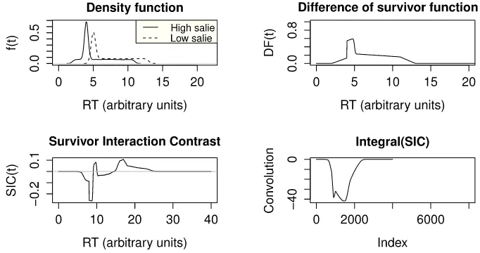
Fig. 3. An example of 2-stage serial exhaustive SIC function that has three 0-crossing points. Graphs include the density functions (top left), the difference of the two corresponding survivor functions (top right), the SIC function (bottom left), and the integral of the SIC function with variable upper limits (bottom right).

We demonstrated the existence of multi-zero SICs by simula-tions. Completion times on processes were generated for both low and high salience regarding the following rules: 1. For simplicity,

we let completion times on processesXandY have the same

dis-tribution form, i.e.,FXL

(t)

=

FYL

(t)

,FXH

(t)

=

FYH

(t)

. ThusDFX

(t)

=

DFY

(t)

. 2. The completion times under the two salience conditions

are both mixtures of uniform and Gaussian distributions with dif-ferent parameters designed so that the two density functions at the

two factor levels cross exactly once and the correspondingDF

(t)

is

unimodal (but not log-concave). The simulation results are shown inFig. 3. The top panel shows the two density functions for the low

and high conditions on the left and theDF(t

)

on the right. The

bot-tom left panel shows the SIC function calculated by taking the dou-ble differences of survivor functions from the top left panel, and the

bottom right panel shows the result of the convolution of

−DF

X

(t)

andDFY

(t)

, which is also the integral of the SIC function, as we

indi-cated in the proof above. As we predicted, the convolution function in the bottom right has three (rather than one) turning points, and corresponding with this is that the SIC function on the left has three 0-crossing points. Also note that in the limit, the convolution func-tion in the bottom right equals 0 as it should, indicating the MIC is still 0 as it should be due to seriality. This simulation supports our finding that when losing the property of log-concavity, the serial exhaustive SIC function may exhibit three non-trivial zeros.

It was intimated in the previous section that the condition of log-concavity is not very restrictive. This claim is supported by con-sidering a simple power function (such as assumed in S.S. Steven’s

famous law):y

=

AxB_{, whereAandBare positive constants,xis the}

independent, andythe dependent variable. ForB

≥

2, this function

is positively accelerated, that is, is convex with the acceleration

increasing withB. Yet, however largeBmay be, it is always

log-concave, since log

(y)

=

log

(A)

+

B

×

log

(x)

which is always

con-cave. And as observed, many commonly used distributions obey this caveat, such as the normal distribution, the exponential

distri-bution, and the gamma distribution with shape parameterP

≥

1,

etc.Proposition 2.2therefore strongly suggests that we should not be astonished to discover a single 0-crossing when processing is serial with an exhaustive stopping rule.

Nonetheless, as mentioned earlier, the SIC has so far been

re-stricted to then

=

2 case. This fact is of more than simple

techni-cal interest, since it has excluded the methodology from the larger numbers of items or processes which are often used in perceptual and cognitive experiments. The next part of this paper is devoted to generalizing the knowledge base of the SIC signatures to arbitrary

values ofn.

3. Fundamental architectural signatures for an arbitrary num-ber of processes

How the two basic architectures, parallel and serial with

vary-ing stoppvary-ing rules behave forn

>

2 processes will be explored in

this section. Before digging into the detail of the extended theory,

we first introduce a measure, which is analogous to the SIC2

(t)

in

Eq.(2), but in a more general form. It will be evident that the

com-plete factorial design can be erected by a recursive embedding in

higher and higher values ofn, as indicated whenn

=

3. The SIC

function of total reaction timeTin 3-process case produces the

ex-pression

SIC3

(t)

= [(S

_LLL

(t)

−

S_LLH

(t

))

−

(S

_LHL

(t

)

−

S_LHH

(t

))]

−[(S

HLL

(t)

−

SHLH

(t))

−

(S

HHL

(t)

−

SHHH

(t))]

(10)

where superscript indicates the number of processes and sub-scripts are used to denote the salience level of each process. For

example,SLLL

(t)

indicates the survivor function of RT for the

con-dition in which all three processes are of low salience. Note that the factorial combination of three factors with their two salience lev-els leads to eight experimental conditions, thus the SIC function in 3-process case is composed of eight items. An abstract form which

is equivalent to Eq.(10)is as follows: SIC3

(t

)

=

∆3_X

1,X2,X3S(t

)

,

whereXirepresents the processi. This form of SIC function can be

straightforwardly generalized to the case for arbitrarynprocesses:

let us denote the individual process asXi,i

=

1

,

2

, . . . ,

n, thus the

SIC function in then-process case could be written as

SICn

(t)

=

∆n_X

1,...,XnS(t

)

(11)

in which∆n_X

1,...,Xnrepresents then-order mixed partial difference

over the factor levels. Analogous to the 3-process SIC which

con-tains 23_{items, then-process SIC function is composed of 2}n

sur-vivor functions.

Now we are ready to present the theoretical results forn

>

2.

Our goal is to demonstrate that for the two major stopping rules, minimum and maximum processing times, the results for arbitrary

nare close relatives to those forn

=

2 in the case for both parallel

and serial systems.12_{Here we employ mathematical induction in}

the proofs. Mathematical induction is usually used to establish that a given statement is true for all non-negative integers. It could be done by proving that the first statement in the infinite sequence

of statements is true, and then proving that if the first N (any arbitrarily chosen number) statements in the infinite sequence of the statements are true, then so is the next one.

We begin with the basic parallel horse race—independent par-allel processing and a minimum time stopping rule.

3.1. Parallel minimum time processing

In the case forn

=

2, the SIC is always positive.Proposition 3.1 reveals that this is the canonical signature for alln.

Proposition 3.1. Assume selective influence. The independent paral-lel minimum time processing predicts that the SIC curve will always be positive as a function of time t, for every n.

Proof. Recall that without the consideration of base time, the to-tal reaction time in parallel minimum time process models should be the minimum of the reaction time on each process i.e,T

=

min

(

TX1

, . . . ,

TXn

)

. Since we assume that two channels process

in-dependently, we have

SICn_par.OR

(

t

)

=

∆n_X1,...,XnP

(

min

(

TX1

, . . . ,

TXn

) >

t

)

=

∆n_X1,...,Xn

[

P

(

TX1

>

t

)

× · · · ×

P

(

TXn

>

t

)

]

(factoring)

= [

P

(

TXnL

>

t

)

−

P

(

TXnH

>

t

)

]

×

∆n_X−_1,...,1 _Xn−1

[

P

(

TX1

>

t

)

× · · · ×

P

(

TX(n−1)

>

t

)

]

= [

FnH

(

t

)

−

FnL

(

t

)

] ×

SICnpar−1.OR

(

t

)

(12)

where subscripts are used to denote the salience level of each pro-cess. For example,TXnLindicates the RT for the condition in which

thenth process is of low salience,FnL indicates the

correspond-ing marginal CDF. Because of the action of selective influence on the survivor functions,FnH

(

t

) >

FnL

(

t

)

for allt. Since SIC2par.OR

(

t

)

is always positive (Townsend & Nozawa, 1995), we can infer that SICn

par.OR

(

t

)

is always positive, by simple mathematical induc-tion.

It is interesting that the sign of the parallel horse race SIC func-tion is always positive asnis varied. We will learn that this does not inevitably occur in a parallel system when considering differ-ent stopping rules. The next proposition treats maximum time par-allel processing.

3.2. Parallel maximum time processing

Whenn

=

2, the SIC function is always negative. From the above proposition with minimum time processing we might ex-pect an analogous invariance with a maximum time (i.e., exhaus-tive processing) stopping rule. Intriguingly, this expectation is not fulfilled as the following proposition reveals.

Proposition 3.2. Assume selective influence. The independent paral-lel exhaustive processing predicts underadditivity in the survivor func-tion when an even number of channels are processed, and predicts overadditivity when an odd number of channels are processed.

Proof. Without the consideration of base time, the total reaction time in parallel exhaustive process models should be the maxi-mum of the reaction time on each process, i.e.,T

=

max

(

TX1

, . . . ,

T_Xn

)

. Thus, we have

SICn_par.AND

(

t

)

=

∆n_X1,...,XnP

(

max

(

TX1

, . . . ,

TXn

) >

t

)

=

∆n_X1,...,Xn

[

1

−

P

(

max

(

TX1

, . . . ,

TXn

)

6t

)

]

= −

∆n_X1,...,XnP

(

max

(

TX1

, . . . ,

TXn

)

6t

)

= −

∆n_X1,...,Xn

[

P

(

TX16t

)

× · · · ×

P

(

TXn6t

)

]

(factoring)

= −[

P

(

TXnL6t

)

−

P

(

TXnH6t

)

]

×

∆n_X−1

1,...,Xn−1

[

P

(

TX16t

)

× · · · ×

P

(

TX(n−1)6t

)

]

= [

FnL

(

t

)

−

FnH

(

t

)

] ×

SICnpar−1.AND

(

t

).

(13)

Because of the action of selective influence on the CDF,FnL

(

t

) <

FnH

(

t

)

for allt. As we know that SIC2par.AND

(

t

)

is negative, we can infer that SICn_par.AND

(

t

)

is negative whennis even and is positive whennis odd.

This flip-flopping of the SIC function according to whethernis odd or even, and only for the exhaustive stopping rule, is quite sur-prising and should be highly useful in identifying mental architec-tures.

We next resume our investigation of serial systems with the same two stopping rules; minimum time first.

3.3. Serial minimum time processing

Recall that in the case of serial processing, a minimum time stopping rule is simplicity itself — the very first completion brings processing to a halt. This simplicity, reinforced with selective in-fluence, extracts a strong result.

Proposition 3.3. Assume selective influence. The independent serial minimum time processing predicts that the SIC will always be zero as a function of time t, for every n.

Proof. The total reaction time in serial minimum time process

models should be the reaction time of the process chosen to be the first one processed. Letpidenote the probability of processing the

ith item first. Then the survivor function on the total reaction time can be expressed as

S

(

t

)

=

P

(

T

>

t

)

=

n



i=1

P

(

T

>

t

|

T

=

TXi

)

×

P

(

T

=

TXi

)

=

n



i=1

pi

×

P

(

TXi

>

t

).

(14)

Due to the complete factorial design, then-process SIC function is composed of 2n_{survivor functions, and all items will cancel each}

other out in the ensuing contrast function. Thus, the minimum time stopping rule leads immediately to a decisive, and invariant prediction.

3.4. Serial maximum time processing

One of the most intriguing architectural signatures of the SIC curve whenn

=

2 is that of serial exhaustive processing, exhibiting as it does the presence of wiggles above and below zero. As we would expect, for arbitraryn, the mean interaction contrast for a serial process with an exhaustive stopping rule must be 0 due to the additivity of the processing times along with selective influence. The following proposition confirms this result using survivor functions but it also follows almost immediately from the foregoing statement.

Proposition 3.4. Assume selective influence. The independent serial exhaustive processing predicts that the integral of the SIC function is always equal to zero, for every n.

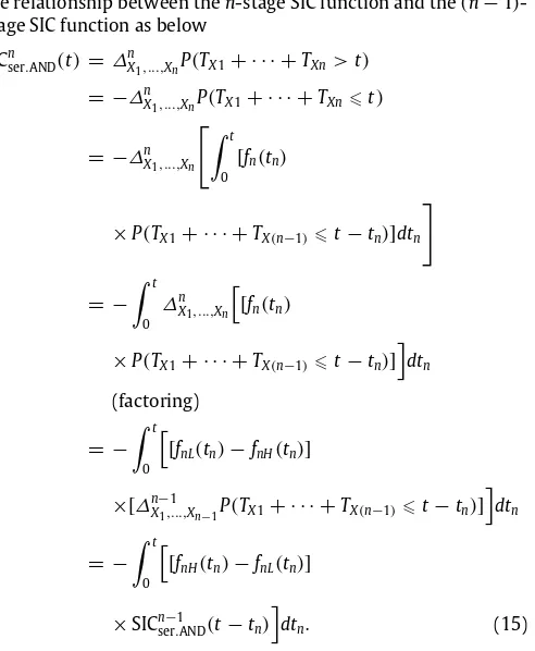
the relationship between then-stage SIC function and the

(

n

−

1

)

-Notice that SICn_ser.AND

(

t

)

is a convolution. By Fubini’s theorem, the integral of the convolution of two functions on the whole space is simply obtained as the product of the integrals of each function, thus the integral of the SIC function on the whole space could be rewritten as

of the above equation is always zero. Thus for everyn, the integral of the SIC function of serial exhaustive model is predicted to be zero.

The next proposition indicates that the SIC function will flip over when the number of processes changes from even to odd and vice versa.

Proposition 3.5. Assume selective influence. The independent serial exhaustive processing predicts that the SIC function must be negative for small times if n is even, and it must be positive for small times if n is odd.

Proof. It is easy to confirm this statement when we examine

the relationship between SIC_sern _.AND

(

t

)

and SIC_sern−_.1_AND

(

t

)

shown in Eq.(15). Notice that the difference between the two density func-tions should be positive for smalltbecause of selective influence at the density crossing level. Thus, whentis small, SICn_ser.AND

(

t

)

and SICn_ser−_.1_AND

(

t

)

have different signs, because of the negative sign be-fore the integral in the above equation.

Propositions 3.4and3.5provide us some key properties of the SIC functions for serial exhaustive models, from which we garner some idea about how the SIC signatures behave, and how they as-sist in identification of the architectures and stopping rules. With regard to the further analysis of SIC curves, recall that in the previ-ous section, we discovered that in then

=

2 case, a mild assump-tion of log-concavity guarantees that there is only a single wiggle through zero. Thus an intriguing question asks how many zeros there will be in SICn

ser.AND

(

t

)

? Is there any trend we can discover as nincreases? The following discussion shows that the answer to all these questions depends on the analytic character of the function. For functions of certain form, the zeros of SICn

ser.AND

(

t

)

will increase

by 1 asnincreases by 1.

Next, it may be remembered that in the previous section we de-termined the zeros of SIC2_ser.AND

(

t

)

via the shape of its integral. Here, we again explore the integral of SICn_ser.AND

(

t

)

for the same purpose. LetIn

₍

_s

₎

_{denote the integral of SIC}n

ser.AND

(

t

)

with variable upper

limit. Eq.(17)reveals the relationship betweenIn

(

s

)

andIn−1

₍

_s

₎

_,

which eventually has the same convolution form as the relation-ship between SIC_sern _.AND

(

t

)

and SIC_sern−_.1_AND

(

t

)

.

Recall that with the assumption of log-concavity,I2

₍

_s

₎

_{is a}

uni-modal function. So following the proof inProposition 2.2, we as-sert thatI3

(

s

)

is a one-wiggle S-shape function, just as SIC2_ser.AND

(

t

)

, ifFX3H

(

t

)

−

FX3L

(

t

)

is strictly log-concave. More generally, with

the assumption of strictly log-concavity ofDFXi, we can infer that In

(

s

)

should have the same key signature as SICn_ser−_.1_AND

(

t

)

by sim-ple math induction. Now the problem of convolution converts to the operation of taking the derivative, that is, how the number of 0-crossings change from SICn_ser−_.1_AND

(

t

)

to SICn_ser.AND

(

t

)

converts to the question of how that number changes when we take the deriva-tive ofIn

(

s

)

. Unfortunately, there appears to be no uniform answer for that question. In fact, for some particular functions such as the Gaussian density function the outcome is pleasant since thenth derivative would havenzeros, which leads to the result that zeros of SICn_ser.AND

(

t

)

will increase by 1 asnincreases by 1.

However, in the general case, the question of the number of zeros of the derivatives could be a quite complicated issue due to the flexible forms of the distributions. As a result, although our hypothesis that zeros would increase by 1 asnincreases has been observed in simulations, theoretical analysis suggests that this hypothesis could be violated, especially whennis a large number.

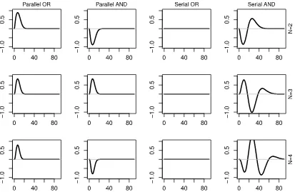
Fig. 4. Predicted survivor interaction contrast forms for Parallel-OR (first column), Parallel-AND (second column), Serial-OR (third column) and Serial-AND (fourth column) processing models, for varyingnfrom 2 to 4 (top to bottom). Simulations are based on Gamma distribution.

4. Exemplary experiment

In a typical short-term memory search task, a small set of items is quickly memorized, and then it is followed by the presentation of a target. Participants are required to indicate, by pressing either the ‘yes’ or ‘no’ button, whether the target was in the memory set. The major interest of the task is to see whether the comparisons of target and memory set items were carried out in serial or in parallel. The data we present below come from an earlier short-term memory search study in which the size of the memory set was manipulated (n

₌

2 or 4). The details of the experiment design and the results forn

₌

2 condition have been reported inTownsend and Fifić(2004), in which they revealed that different individuals may evince either parallel or serial processing. In this paper we take one participant whose data in then

₌

2 condition strongly support serial processing for example, and we focus on his data in then

₌

4 condition. With a larger memory set of size 4, we might expect to see more and consistent evidence to support serial processing. Then

₌

4 design also allows for examination of wiggle behavior of the observed SIC functions.

4.1. Method

The task was carried out in Belgrade, using stimuli crafted from Serbian linguistic features. Five participants were recruited for the experiment. Each participant participated in both then

₌

2 and n

₌

4 conditions. A total of 12 stimuli were constructed and they were all pseudo Serbian words in consonant–vowel–consonant form. In the experiment, each trial consisted of a fixation point and warning low-pitch tone for 1 s, successive presentation of two or four items in the memory set for 1200 ms, an interstimulus interval (ISI), and a target. Participants were required to indicate, by pressing either the ‘yes’ or ‘no’ button, whether the target was in the memory set or not. The ISI was also manipulated, ISI

₌

700 or 2,000 ms. In then

₌

4 task, participants were run for 44 blocks of 128 trials for each ISI condition, and they were required to respond as fast as they could without compromising accuracy. Target items

and memory-set items were manipulated across trials to produce low and high levels of item-target dissimilarity. For examples of stimuli and more details on the experimental setup, seeTownsend and Fifić(2004).

4.2. Data analysis

Our analyses focused only on target-absent trials. As in

Townsend and Fifić(2004), the experimental factor for each dis-tractor item (which coincided with a stage in serial processing or a channel in parallel processing) was its similarity to the target. This type of manipulation should permit selective influence on exhaustive (‘no’) trials but could introduce confounds on single-target, self-terminating (‘yes’) trials. Naturally, on target-absent trials, participants must exhaustively process all four comparisons of target and memory set items to guarantee a correct response.

To implement the double factorial paradigm, we conducted two levels of item-target dissimilarity. High dissimilarity was desig-nated as the high salience condition and low dissimilarity was des-ignated as the low salience condition. Thus the factors of interests were positions of item in the set (1, 2, 3, 4)

_×

phonemic similarity (low, high). The factorial combination of four factors with their two salience levels leads to sixteen experimental conditions (2

_×

2

_×

2

_×

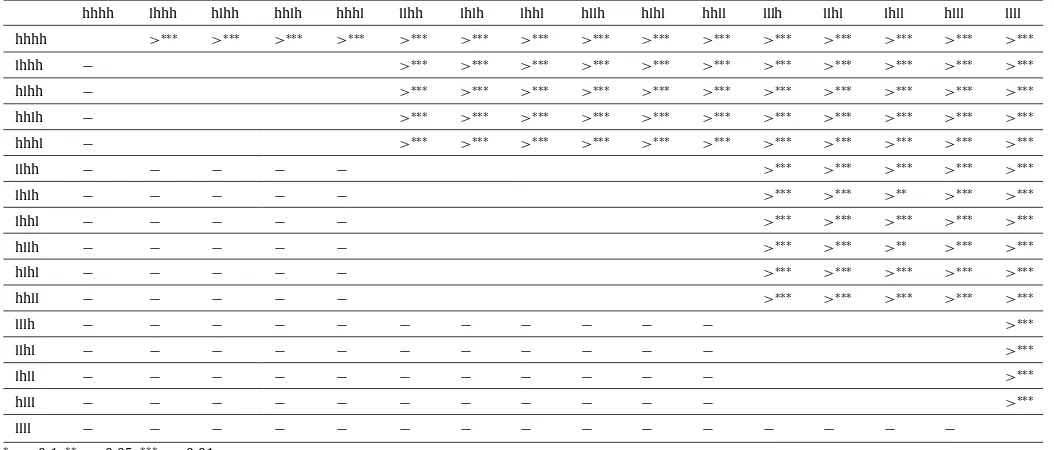
2). For instance, LHHH indicates a condition in which the first factor is of low salience and all other factors are of high salience. Simpler embedded factorial designs can be derived from the full design by reducing the number of factors. For instance, from the four-target design it is possible to obtain 4 three-target designs, by dropping out any of the positional factors. Thus, the following will be obtained: x234, 1x34, 12x4 and 123x. The ‘x’ denotes posi-tion that was dropped out from the analysis. Similarly, excluding yet another factor would derive 6 two-target designs: xx34, x2x4, x23x, 1xx4, 1x3x, 12xx. In other words, merging selected factors allow us to analyze the underlying architecture of any two, three or four mental processes within one experiment.

Table 1

Results of the Kolmogorov–Smirnov test applied to the full task.

hhhh lhhh hlhh hhlh hhhl llhh lhlh lhhl hllh hlhl hhll lllh llhl lhll hlll llll

hhhh >∗∗∗ _>∗∗∗ _>∗∗∗ _>∗∗∗ _>∗∗∗ _>∗∗∗ _>∗∗∗ _>∗∗∗ _>∗∗∗ _>∗∗∗ _>∗∗∗ _>∗∗∗ _>∗∗∗ _>∗∗∗ _>∗∗∗

lhhh − >∗∗∗ _>∗∗∗ _>∗∗∗ _>∗∗∗ _>∗∗∗ _>∗∗∗ _>∗∗∗ _>∗∗∗ _>∗∗∗ _>∗∗∗ _>∗∗∗

hlhh − >∗∗∗ _>∗∗∗ _>∗∗∗ _>∗∗∗ _>∗∗∗ _>∗∗∗ _>∗∗∗ _>∗∗∗ _>∗∗∗ _>∗∗∗ _>∗∗∗

hhlh − >∗∗∗ _>∗∗∗ _>∗∗∗ _>∗∗∗ _>∗∗∗ _>∗∗∗ _>∗∗∗ _>∗∗∗ _>∗∗∗ _>∗∗∗ _>∗∗∗

hhhl − >∗∗∗ >∗∗∗ >∗∗∗ >∗∗∗ >∗∗∗ >∗∗∗ >∗∗∗ >∗∗∗ >∗∗∗ >∗∗∗ >∗∗∗

llhh − − − − − >∗∗∗ _>∗∗∗ _>∗∗∗ _>∗∗∗ _>∗∗∗

lhlh − − − − − >∗∗∗ >∗∗∗ >∗∗ >∗∗∗ >∗∗∗

lhhl − − − − − >∗∗∗ _>∗∗∗ _>∗∗∗ _>∗∗∗ _>∗∗∗

hllh − − − − − >∗∗∗ _>∗∗∗ _>∗∗ _>∗∗∗ _>∗∗∗

hlhl − − − − − >∗∗∗ >∗∗∗ >∗∗∗ >∗∗∗ >∗∗∗

hhll − − − − − >∗∗∗ _>∗∗∗ _>∗∗∗ _>∗∗∗ _>∗∗∗

lllh − − − − − − − − − − − >∗∗∗

llhl − − − − − − − − − − − >∗∗∗

lhll − − − − − − − − − − − >∗∗∗

hlll − − − − − − − − − − − >∗∗∗

llll − − − − − − − − − − − − − − −

∗_p<0.1;∗∗_p<0.05;∗∗∗_p<0.01

>∗∗∗_{: max(F}

HHHH(t)−FLHHH(t))is significant,p<0.01, etc. −: max(FLHHH(t)−FHHHH(t))is not significant, etc.

the ISI between memory-set presentation and the probe. However, all the SIC functions decisively adhered to either a serial or paral-lel form. To demonstrate the use of the new theories for revealing architecture for multiple processes, we take one participant (Par-ticipant 1 inTownsend and Fifić(2004)) whose data consistently support serial processing as an example of our new theoretical re-sults. We were therefore curious to examine behavior for larger n, particularly since most memory search experiments are based onn

>

2. We were also keen to test the within-architecture pre-dictions concerning behavior as the number of processes altered acrossn

₌

2

,

3

,

4, utilizing the above ‘factor reduction’ strategy.

Evidence of selective influence was first assessed by a two-sample Kolmogorov–Smirnov test. As noted earlier, selective influ-ence implies that the reaction time when the target is low saliinflu-ence is stochastically larger than the reaction time when the target is high salience. In other words, it implies that the distribution func-tions of RT should exhibit a stochastic ordering across condifunc-tions. In the two-sample Kolmogorov–Smirnov test, the null hypothesis is that the two empirical distributions are equal, and the alternative hypothesis is that the two distributions are different, in the sense that the maximum of the difference between two distributions is significantly large. To test for illegitimate cumulative distribu-tion funcdistribu-tion crossings (logically equivalent to crossings of the sur-vivor functions), we applied the one-sided Kolmogorov–Smirnov test twice on each pair of conditions to assess selective influence as is common practice (e.g.,Townsend & Nozawa, 1995). For in-stance, when assessing the selective influence between the con-ditions HHHH and HHHL, we require that max

(

FHHHH

−

FHHHL

)

is

significant and max

(

F_HHHL

₋

F_HHHH

)

is not significant.

Next, the architecture and stopping rule first assessed by the adjusted rank transform (ART;Sawilowsky(1990)) test. The ART test is a nonparametric test for an interaction between two discrete variables. We apply it to distinguish serial versus parallel mod-els. The null hypothesis is that there is no interaction between the salience manipulations on each process, so rejecting the null hy-pothesis falsifies serial models

(

MIC

₌

0

)

. The architecture and stopping rule were additionally examined by a nonparametric sta-tistical test of SIC, which was recently developed byHoupt and Townsend(2010). This test performs two separate null hypothe-sis tests with a D-statistic: One is for testing whether the empirical

SIC function (ESIC) has a significant positive deviation from zero, and the other is pertinent to testing whether the ESIC has a signifi-cant negative deviation from zero. Referring toFig. 1, rejecting the null hypothesis of the first test falsifies serial-OR and parallel-AND models, whereas rejecting the null hypothesis of the second test falsifies serial-OR and parallel-OR models. It may be observed that the significance test of SIC function cannot presently distinguish a serial-AND model from a coactive model, since both models are expected to have a significant positive deviation and a significant negative deviation. Thus combining the statistical test of SIC with the ART test is necessary. For more details of the statistical test of SIC, seeHoupt and Townsend(2010).

4.3. Result

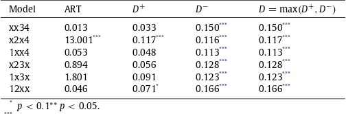
Selective influence. The Kolmogorov–Smirnov tests were ap-plied to each pair of high versus low salience conditions in the full task.Table 1shows the K–S results for the participant: As shown inTable 1, in every case where an order was predicted, the appro-priate ordering was supported, either at thep

₌

0

.

01 orp

₌

0

.

05 level. Additionally, non-significant results were found for each pair of conditions with the application of the inverse direction.

Architecture and stopping rule. The empirical SIC (ESIC) func-tions for the same participant are plotted inFig. 5. The top figure displays the four-target ESIC function (n

₌

4), the middle row shows four reduced three-target ESICs (n

₌

3), and the bottom row of theFig. 5shows a total of 6 two-target ESICs (n

₌

2). The statis-tical tests were applied to analyze then

₌

2 ESIC functions, with results summarized inTable 2. The first column inTable 2shows the statistical results of the ART test, and the rest of the table ex-hibits the maximum deviations from the statistical test of ESIC.

Fig. 5. ESIC(t)for one participant. The top row is the ESIC for the original 4-target task. The middle and bottom rows are the ESICs estimated from the reduced 3-target and 2-target tasks, respectively.

Table 2

Results of the SIC and the ART test statistics applied to the data from the reduced 2-target tasks.

Model ART D+

D−

D=max(D+

,D−

)

xx34 0.013 0.033 0.150*** _0.150***

x2x4 13.001*** _0.117*** _0.116*** _0.117***

1xx4 0.053 0.048 0.113*** _0.113***

x23x 0.894 0.056 0.128*** _0.128***

1x3x 1.801 0.091 0.123*** _0.123***

12xx 0.046 0.071* _0.166*** _0.166***

*_{p<0.1**p<0.05.}

***_p<0.01.

exhibiting a significant result of the ART test, which implies a possible interaction between processes 2 and 4. Since bothD+_and D−

are significant from zero (D+

=

0

.

117,D−

=

0

.

116,p

<

0

.

01), unfortunately we cannot rule out the coactive model as a model of processing in this case (seeFig. 1, right panel).

The current SIC statistical tests for significance are limited by their confinement ton

=

2. Forn

>

2, however, even without sta-tistical tools, we can nevertheless assay the qualitative form of the ESIC signatures. In fact, as we can see, the signatures of ESIC when n

=

3 exhibits clear M-shaped patterns. Each ESIC was positive for early processing times and negative in the middle, and go up again for the later processing times. Those M-shaped patterns provide preliminary evidence for a three-stage serial AND processing. The top 4-target ESIC function appears to cross thex-axis at least twice although crossings at the tail are rather minuscule. The 4-target ESIC function does start negative, and then becomes positive, and then appears to wiggle.

Moreover, for each of the ESIC functions we observed equal pos-itive and negative areas, confirming the prediction of serial AND model. Intriguingly, the ESIC functions further appear to obey the flip-flopping property when the number of processes changes from even to odd. Thus we tentatively infer that this participant searches her/his short-term memory serially for up to 4 memory items.

5. Summary and discussion

This paper expands the knowledge base concerned with identi-fication of the simple but crucial architectures referred to as serial and parallel processing along with two major decisional stopping rules. As in almost all of our developments on these topics, the pre-dictions have been entirely distribution free. This attribute renders the related diagnostic tests more robust and permits the testing

(e.g., falsification) of entire classes of models. The present devel-opments continue that tradition.

The SIC behavior of parallel processing in league with the ma-jor stopping rules and forn

=

2, has been definitively established since 1995 (Townsend & Nozawa, 1995). Likewise, minimum pro-cessing time serial signatures were already known for n

=

2. However, in the important case of serial exhaustive processing, the exact form of the SIC signature has been unclear, even forn

=

2. The early results showed that it must start negative (i.e., for small time values,t), express positive areas as well and that the positive plus negative areas must equal zero. Many simulations and some experimental data (Fific, Little, & Nosofsky, 2010;Fific, Nosofsky, & Townsend, 2008;Little, Nosofsky, & Denton, 2011;Townsend & Fi-fić, 2004) further have suggested a single 0-crossing but this prop-erty had not been proven.

The present investigation thus began by exploring the precise behavior of the serial exhaustive SIC function forn

=

2. We found that a single wiggle (i.e., one 0-crossing) cannot be absolutely guaranteed since there exist probability distributions that do not elicit that property. However, it was proven that: A. There must be an odd number of crossings for any distributions. B. A rather mild condition known as log-concavity is sufficient as a guarantor of a single 0-crossing.

Up until now, there has further been a lack of knowledge concerning how the architectural signatures act whennis varied. The second major part of the investigation pursued this issue. The present theoretical analysis provides this information for parallel and serial models in conjunction with both the minimum time and maximum time stopping rules. Although in some cases the exact shape of the SIC curve is still unknown (e.g., the SIC for the serial exhaustive model forn

>

2) due to the flexibility of distribution forms of the processing time, we have provided thorough analysis specifying critical and differing traits of SIC functions under different models that should prove vital in identifying fascinating these elementary, but fundamental, architectures along with their stopping rules.

The present developments significantly expand the arena within which SFT and RT data can assay elementary architectures and stopping rules and we anticipate their application in basic and applied research.

Acknowledgments