www.elsevier.com/locate/econedurev
Family background and returns to schooling in Taiwan
Jin-Tan Liu
a,*, James K. Hammitt
b, Chyongchiou Jeng Lin
caDepartment of Economics, National Taiwan University, 21 Hsu-Chow Road, Taipei (100), Taiwan
bCenter for Risk Analysis and Department of Health Policy and Management, School of Public Health, Harvard University, 718
Huntington Avenue, Boston, MA 02115, USA
cSchool of Public Health, University of Pittsburgh, 130 Desoto Street, Pittsburgh, PA 15261, USA Received 24 July 1998; accepted 17 December 1998
Abstract
Estimated returns to schooling in Taiwan are sensitive to the inclusion of family background variables in the wage function. The effects of family background on worker’s wage are significant in the private sector but not in the public sector, suggesting that wages are more sensitive to unobserved ability or family connections in the private sector than in the public sector. The estimated wage function is convex; returns to schooling increase with the level of education. The effect of father’s schooling is larger than the effect of mother’s schooling in the wage function; however, the effect of wife’s schooling is even larger. These results suggest that estimates obtained without controlling for family background may be biased upward, reflecting unobservable worker characteristics and assortative mating behavior. Analysis of the potential role of measurement error bias suggests that inclusion of family background variables may overstate by one third the extent to which omission of family background variables affects the returns to schooling. [JEL J12, J24]1999 Elsevier Science Ltd. All rights reserved.
Keywords: Family background; Return to schooling
1. Introduction
Previous empirical research has found that private returns to schooling are often high in developing coun-tries (Psacharopoulos, 1985; Schultz, 1988).1 However,
apparent returns to schooling may be biased upward by omission of important variables such as ability and fam-ily background. Since it is not easy to measure ability directly, many studies examine the impact of family background on wages. Family background can be a
* Corresponding author. Tel.: 2351-9641; fax: 886-2-2321-5704; e-mail: [email protected]
1According to Psacharopoulos’s survey, the average esti-mated rate of return from Mincer-type earnings or wage func-tions is inversely related to the level of economic development. The average estimated rate of return is 18% for Latin America, 12.8% for Asia, 13.4% for Africa and 7.7% for advanced coun-tries.
0272-7757/99/$ - see front matter1999 Elsevier Science Ltd. All rights reserved. PII: S 0 2 7 2 - 7 7 5 7 ( 9 9 ) 0 0 0 2 5 - 4
relationship between children’s education and earnings may overstate the effect of education on labor pro-ductivity.
Most studies of the effects of family background on earnings in developing countries have focused on Latin American countries, where intergenerational economic mobility is known to be low (Strauss & Thomas, 1995). In an early study, Carynoy (1967) found that father’s occupation had a strong influence on wages of males in Mexico. Heckman and Hotz (1986) added the education of the worker’s mother and father in earning functions for Panamanian men. They found parents’ education has a positive effects on earnings, with the mother’s edu-cation having the larger effect. The estimated returns to own education fall by 25% when family background is included in the estimation. Behrman and Wolfe (1984) estimated a household income function for adult women in Nicaragua, using parental education as control vari-ables, and found a significant positive effect of father’s schooling. Stelcner, Arriagada and Moock (1987) found similar results in a study of Peru. Lam and Schoeni (1993) studied the Brazilian labor market and found not only an effect of parents’ education, but also an effect of education of the spouse’s parents. The effect of the spouse’s father’s education is even greater than the effect of the respondent’s own father. They also found that marginal returns increase with higher levels of parental schooling.
Studies outside of Latin America have also shown the importance of family background factors. Sahn and Alderman (1988) studied the Sri Lanka labor market and found that father’s wage has a positive effect on the son’s wage. Armitage and Sabot (1987) used data from Kenya and Tanzania and found that marginal returns to own schooling rise sharply with parents’ schooling. In contrast, Ozdural (1993) found that parents’ education is important for the quantity of education children receive but has no further impact on earnings of Turkish men.
In this paper, we examine the effects of family back-ground on the wage function in Taiwan. Among developing countries, Taiwan has one of the highest degrees of earning equality (Fei, Ranis & Kuo, 1979). The data are from the 1990 Taiwan Human Resource Utilization Survey, the annual household survey conduc-ted by the Directorate-General of Budget, Accounting and Statistics, Taiwan. We analyze the married male sample. In the empirical analysis we estimate a series of wage equations in which we include various combi-nations of the schooling of the worker and schooling of the worker’s father, mother, and wife. We separate the sample into public sector and private sector employees. Our conclusions are as follows. First, we find direct effects of family background on wages in the private sec-tor but not in the public secsec-tor. One possible explanation is that the public sector is more meritocratic and that nepotism and family connections are more influential in
the private sector.2
Alternatively, family connections may be influential in obtaining access to public-sector employment, but have a smaller quantitative effect on public sector wages than on private sector wages because public sector wages are less variable or less sensitive to productivity differences. Second, we compare effects of the father’s and of the mother’s education after we con-trol for the worker’s own schooling. The results suggest that the father’s education is more important than the mother’s, which differs from the findings of Heckman and Hotz (1986) for Panamanian men. Third, we find that the wife’s schooling has a larger effect on a worker’s wage than the schooling of the worker’s own parents. This suggests a role for assortative mating, as more edu-cated women may choose to marry men with higher earning potential. It also suggests that male workers may receive support from their wife’s parents. Assuming the wife’s education is correlated with her parent’s edu-cation, the parents of a well-educated wife may be more able to assist their son-in-law in obtaining a desirable job (in the extreme case, by hiring him into their firm). Finally, we find the potential role of measurement error in schooling may explain part of the decrease in returns to schooling when family background variables are included.
The remainder of the paper is organized as follows. Section 2 briefly presents the data and describes the sam-ple characteristics. Section 3 introduces the empirical models, while Section 4 discusses the empirical results. The final section provides the summary and conclusion.
2. Data and sample characteristics
The data for this analysis are taken from the 1990 Tai-wan “Human Resource Utilization Survey”. In this sur-vey, all adults aged 16 years and older in each selected household were interviewed. We restrict our analysis to married male (non-agricultural) workers living in the same household as their parents.3 The final sample
includes 1082 married male workers, of whom 135 are employed in the public sector and 947 in the private
sec-2The private sector labor market in Taiwan appears to be highly competitive, as it is composed of many small firms with little intervention by unions or government (e.g. minimum wage laws, labor codes) (Fields, 1992; Hou, 1993). This suggests the higher private-sector returns to education reflect ability more than family connections.
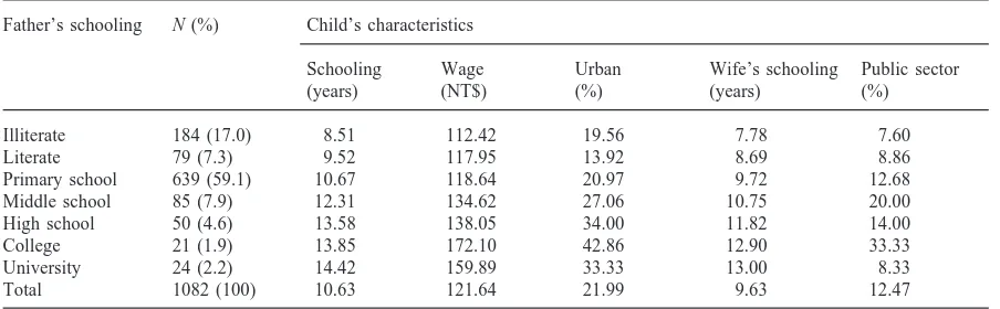
Table 1
Characteristics of respondent by father’s schooling (full sample) Father’s schooling N (%) Child’s characteristics
Schooling Wage Urban Wife’s schooling Public sector
(years) (NT$) (%) (years) (%)
Illiterate 184 (17.0) 8.51 112.42 19.56 7.78 7.60
Literate 79 (7.3) 9.52 117.95 13.92 8.69 8.86
Primary school 639 (59.1) 10.67 118.64 20.97 9.72 12.68
Middle school 85 (7.9) 12.31 134.62 27.06 10.75 20.00
High school 50 (4.6) 13.58 138.05 34.00 11.82 14.00
College 21 (1.9) 13.85 172.10 42.86 12.90 33.33
University 24 (2.2) 14.42 159.89 33.33 13.00 8.33
Total 1082 (100) 10.63 121.64 21.99 9.63 12.47
tor.4The survey reports the worker’s schooling and the
schooling of parents and wife as one of eight categories: illiterate, literate (self-taught), completed primary school (6 years), middle school (9 years), high school (12 years), college (15 years without bachelor degree), uni-versity (16 years with bachelor degree), and graduate school (with master’s degree or higher). Unlike the data used in Lam and Schoeni (1993, 1994), our data do not include educational information on parents-in-law of respondents, so it is impossible to compare the effects between parents and parents-in-law.
Table 1 summarises the characteristics of respondents by father’s schooling for the sample. Approximately 60% of the labor force has father’s schooling at the level of primary school. The wage rate is the ratio of monthly earnings from the primary job divided by four times the number of hours worked per week. The mean hourly wage is NT$121.64.5The mean years of schooling for
fathers, mothers and workers are 5.45, 2.89 and 10.63 years, which indicates a substantial increase in schooling across generations. Lam and Schoeni (1993, 1994) report the mean schooling of male workers in Brazil in 1982 was only 4.34 years, compared with 13.4 years in the U.S. in 1988. According to their study, 39% of married Brazilian males aged 30–55 have illiterate fathers. In contrast, only 17% of our sample have illiterate fathers. Mean schooling for wives is slightly less than for hus-bands overall and in each of the separate groups defined by father’s education. The correlation between husband’s and wife’s schooling is 0.63, which is lower than in the Brazilian labor market but higher than in the U.S. labor market (Lam & Schoeni, 1994). This statistic suggests a
4The division of sample workers between the public and private sectors (12% and 88%, respectively) mirrors the division of the overall Taiwanese labor market (Hou, 1993).
5The 1990 exchange rate was US$15 NT$27.1075 (New Taiwan Dollars).
high degree of assortative mating by schooling in Tai-wan.
Correlation between the education or earnings of two generations can be due to cultural inheritance, govern-ment education policies, or capital market constraints on borrowing to finance education. The correlations of schooling are 0.44 for child and father and 0.35 for child and mother. These correlations are lower than the find-ings for Panama in Heckman and Hotz (1986), but are close to the findings in the U.S. and Turkey (Blau & Duncan, 1967; Ozdural, 1993).6The correlations imply
that father’s education may play a more important role in affecting children’s years of schooling than mother’s education.
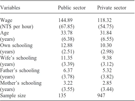
Table 2 reports the basic statistics of wage and school-ing variables in the public and private sectors. The mean wage of the public sector employees, NT$144.89, is larger than the mean wage of the private sector employees, NT$118.21. Similarly, the years of schooling of workers, parents, and wives in the public sector are all greater than those in the private sector. Compared with all male workers, our subsample is younger (about one standard deviation) and slightly more educated and higher paid.7
6The schooling correlations in Heckman and Hotz (1986) are 0.57 for father and son, 0.75 for mother and son, 0.68 for grandfather and father. The schooling correlations in Ozdural (1993) are 0.42 for father and child or mother and child in the U.S., 0.46 for father and child, 0.33 for mother and child in Tur-key.
7For the full sample of public-sector employees (n53558), mean age539.12, own years of schooling512.31, and wage
5NT$141.05. For the full sample of private-sector employees (n5 17 447), mean age5 39.25, own years of schooling5
Table 2
Basic statistics of public and private sector employeesa Variables Public sector Private sector
Wage 144.89 118.32
(NT$ per hour) (67.85) (54.75)
Age 33.78 31.84
aNote: Standard deviations are in parentheses.
3. Empirical models
In the empirical analysis below we follow the model outlined in Lam and Schoeni (1993, 1994). We estimate a series of wage equations in which we begin with the schooling of the worker and socioeconomic variables as regressors, and sequentially add the schooling of the worker’s father, mother, and wife. These regressions pro-vide statistical tests for the role of family background in explaining returns to schooling in Taiwan. To examine possible differences between the wage structures of the public sector and the private sector, we estimate the model for the full sample first, then separate the sample into public and private sector subsamples.
The wage equation takes the general form:
yi5lnWi5b01bsSi1baAi1ui (1)
where lnW is the log of the wage, Siis years of
school-ing, Ai is an unobservable variable that affects wages,
such as ability, and uiis an error term distributed
inde-pendently of Siand Ai. Suppose that ability has positive
returns in the labor market and is positively correlated with schooling. Two kinds of estimation bias may exist in the wage function, omitted-variable bias and measure-ment-error bias. We discuss the omitted-variable bias first. Assume the worker’s ability is positively correlated with family background variables, for which parents’ schooling, Fi, serves as an index. Further, assume ability
can be expressed as a linear function of parents’ edu-cation:
Ai5afFi1A
u
i (2)
Eq. (2) decomposes ability into two components, an ‘inherited’ component, afFiand an ‘uninherited’
compo-nent, Au
Eq. (3) shows that parental education Fiis an indicator
of inherited unobserved variables omitted from the wage regression. If the variables are correlated with the work-er’s schooling, inclusion of family background variables will reduce the omitted-variable bias in the estimated return to schooling. Similarly, given returns to family connections, the inclusion of parental schooling will decrease the estimated return to own schooling. If we include the wife’s schooling in the husband’s wage equ-ation, we can expect it to also have a positive coefficient and to decrease returns to own schooling as long as there is a positive assortative mating with respect to ability or social connections.
A second econometric issue is measurement error in the reported schooling variable (Griliches, 1977). Assume S*is the true (unobserved) schooling, and the
observed schooling S5S*1e, with e random and
inde-pendent of S*. Letl 5Var(e)/Var(S) represent the
noise-to-signal ratio in schooling. The probability limit of the estimated coefficient in an OLS regression of wages on
S,bs, is
Plimbs5bs2bsl 1 babas(12l) (4)
where bas is the coefficient from a regression of true
ability on true schooling. The second term is the down-ward bias due to measurement error in schooling. The third term is due to the omitted ability variable and will be positive if schooling and ability are positively corre-lated.
As shown by Lam and Schoeni (1993), when family background Fi is included in the wage regression, the
probability limit of the estimated return to schooling is
Plimbs5bs2bs
sf is the R2from a regression of own schooling
on family background and other variables, andr2 afis the
4. Empirical results
4.1. Effects of parental background
Our major interest is how returns to schooling are affected by considering various family members’ edu-cational backgrounds. To analyze the relationship between worker’s wages and schooling, we estimate a series of wage equations with and without controls for parental and/or spousal education. Ordinary least-squares (OLS) estimates are reported in Tables 3–5. Table 3 presents the results for the full sample; Tables 4 and 5 present results for the public sector and the private sector respectively. In all cases, we find strong evidence that omitted-variable bias increases estimated returns to
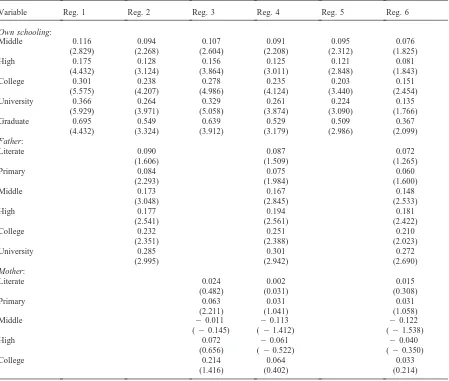
Table 3
Wage equations estimation in the full sample (OLS). Dependent variable: log of hourly wagea
Variable Reg. 1 Reg. 2 Reg. 3 Reg. 4 Reg. 5 Reg. 6
Own schooling:
Middle 0.116 0.094 0.107 0.091 0.095 0.076
(2.829) (2.268) (2.604) (2.208) (2.312) (1.825)
High 0.175 0.128 0.156 0.125 0.121 0.081
(4.432) (3.124) (3.864) (3.011) (2.848) (1.843)
College 0.301 0.238 0.278 0.235 0.203 0.151
(5.575) (4.207) (4.986) (4.124) (3.440) (2.454)
University 0.366 0.264 0.329 0.261 0.224 0.135
(5.929) (3.971) (5.058) (3.874) (3.090) (1.766)
Graduate 0.695 0.549 0.639 0.529 0.509 0.367
(4.432) (3.324) (3.912) (3.179) (2.986) (2.099)
Father:
Literate 0.090 0.087 0.072
(1.606) (1.509) (1.265)
Primary 0.084 0.075 0.060
(2.293) (1.984) (1.600)
Middle 0.173 0.167 0.148
(3.048) (2.845) (2.533)
High 0.177 0.194 0.181
(2.541) (2.561) (2.422)
College 0.232 0.251 0.210
(2.351) (2.388) (2.023)
University 0.285 0.301 0.272
(2.995) (2.942) (2.690)
Mother:
Literate 0.024 0.002 0.015
(0.482) (0.031) (0.308)
Primary 0.063 0.031 0.031
(2.211) (1.041) (1.058)
Middle 20.011 20.113 20.122
(20.145) (21.412) (21.538)
High 0.072 20.061 20.040
(0.656) (20.522) (20.350)
College 0.214 0.064 0.033
(1.416) (0.402) (0.214)
Continued.
schooling in the full sample and the private sector, but not in the public sector.
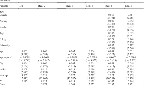
Table 3 Continued
Variable Reg. 1 Reg. 2 Reg. 3 Reg. 4 Reg. 5 Reg. 6
Wife:
Literate 0.565 0.581
(2.194) (2.265)
Primary 0.609 0.592
(5.387) (5.230)
Middle 0.597 0.577
(5.071) (4.896)
High 0.702 0.675
(5.882) (5.651)
College 0.779 0.746
(5.987) (5.724)
University 0.807 0.787
(5.708) (5.540)
Age 0.065 0.066 0.065 0.066 0.049 0.051
(4.299) (4.383) (4.332) (4.386) (3.227) (3.352)
Age squared 20.0008 20.0008 20.0008 20.0008 20.0005 20.0006
(23.786) (23.847) (23.803) (23.852) (22.438) (22.563)
City 0.064 0.060 0.065 0.064 0.049 0.049
(2.106) (1.970) (2.115) (2.081) (1.615) (1.614)
Public 0.108 0.116 0.113 0.116 0.096 0.104
(2.693) (2.893) (2.798) (2.848) (2.408) (2.603)
Intercept 3.307 3.228 3.277 3.222 2.923 2.859
(12.445) (12.067) (12.287) (11.999) (10.754) (10.420)
R2 0.113 0.127 0.118 0.131 0.145 0.164
F-test 2.973 1.368 2.052 7.535 3.821
aNotes: t-statistics are in parentheses. Sample sizes are 1082. F-test: null hypothesis is that all family background schooling coefficients equal zero.
schooling of the worker’s mother to regression 1. Regression 4 includes the schooling of both parents. Regression 5 adds the wife’s schooling only. Regression 6 includes the worker’s wife’s and parents’ schooling together. The explanatory power (R2) of all models in
Table 3 is about 0.15. It rises very little as we add differ-ent kinds of family background variables (from 0.113 in the first regression to 0.164 in the last).
We begin with regression 1 of Table 3, which includes only the worker’s own schooling. Compared with a worker with primary schooling, the estimated returns to schooling are 12% for completion of middle school, 19% for high school, 35% for college, 44% for university, and 104% for graduate school.8The estimated wage function
is convex and so returns to schooling increase with the level of education. This result is consistent with findings in Brazil (Strauss & Thomas, 1994) and Cote d’Ivoire (van der Gaag & Vijverberg, 1989), but is inconsistent with the survey in Psacharopoulos (1985). Psacharo-poulos found primary education to be the most profitable
8From the coefficient in regression 1 of Table 3, a university-educated worker implies a wage that is e0.36651.44 times the wage of a worker with only primary schooling.
educational investment, followed by middle school and high school. This convexity may reflect differences in unobserved characteristics of individuals who choose to continue to higher levels of education.9The results are
also consistent with a strong ‘diploma effect’ or ‘sheep-skin effect’ associated with completion of college, uni-versity and graduate school (Hungerford & Solon, 1987; Dougherty & Jimmenez, 1991). Similar effects have been found in Brazil (Lam and Schoeni, 1993) and Cote d’Ivoire (van der Gaag & Vijverberg, 1989).
To separate the effects of father’s and mother’s edu-cation on their child’s rates of return to schooling, we include father’s and mother’s educational background separately. The omitted category is illiterate. Regression 2 of Table 3, which includes the worker’s father’s schooling, shows a significant wage advantage with a better educated father. When we control for the worker’s own schooling, having a university-educated father implies a 33% wage advantage over an illiterate father. All the coefficients of father’s schooling variables are statistically significant except literate. In comparison to
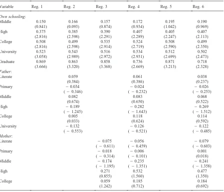
Table 4
Wage equations estimation in the public-sector sample (OLS). Dependent variable: log of hourly wagea
Variable Reg. 1 Reg. 2 Reg. 3 Reg. 4 Reg. 5 Reg. 6
Own schooling:
Middle 0.150 0.166 0.157 0.172 0.195 0.190
(0.841) (0.093) (0.874) (0.934) (1.042) (0.969)
High 0.375 0.385 0.390 0.407 0.405 0.407
(2.816) (2.598) (2.291) (2.289) (2.247) (2.113)
College 0.508 0.499 0.535 0.524 0.508 0.499
(2.816) (2.598) (2.914) (2.719) (2.590) (2.350)
University 0.523 0.543 0.516 0.534 0.512 0.502
(3.058) (2.989) (2.972) (2.931) (2.699) (2.473)
Graduate 0.869 0.863 0.858 0.736 0.871 0.718
(3.666) (3.320) (3.368) (2.669) (3.213) (2.328)
Father:
Literate 0.059 0.061 0.038
(0.384) (0.386) (0.237)
Primary 20.034 20.024 20.026
(20.346) (20.232) (20.253)
Middle 0.082 0.083 0.068
(0.674) (0.650) (0.522)
High 20.189 20.282 20.269
(21.245) (21.643) (21.512)
College 0.005 0.118 0.114
(0.033) (0.624) (0.592)
University 20.132 20.126 20.122
(20.553) (20.521) (20.485)
Mother:
Literate 20.075 20.056 20.079
(20.611) (20.459) (20.603)
Primary 20.018 20.006 0.001
(20.314) (20.101) (0.018)
Middle 20.174 20.235 20.241
(21.195) (21.351) (21.358)
High 0.271 0.532 0.477
(0.855) (1.560) (1.350)
College 0.059 0.185 0.184
(1.242) (0.712) (0.692)
Continued.
the results in regression 1, the estimated coefficients of own schooling in regression 2 drop by 19% for middle school, 27% for high school, 21% for college, 28% for university, and 21% for graduate school.
In contrast, most estimated coefficients of mother’s schooling (regression 3 of Table 3) are not statistically significant except at the level of primary school and the partial effects of the mother’s education are not jointly significant (F 5 1.368). In comparison with the regression 1 estimates, average returns to own schooling decline slightly. For example, the coefficients of own schooling drop only 8% for middle school and for gradu-ate school. When both parents’ education are included simultaneously (regression 4), the partial effect of the father’s education exceeds that of the mother’s education at all levels. This result contrasts with previous studies.
Behrman and Wolfe (1984) for the earnings of Nicarag-uan females, and Heckman and Hotz (1986) for Pana-manian males, both found that mother’s schooling has a greater effect on earnings than father’s schooling. Lam and Schoeni (1993) found a mixed result regarding the relative effects of father’s and mother’s schooling on child’s earnings.10In contrast, our finding that father’s
schooling has a larger effect on son’s earnings than does mother’s schooling is consistent with the social structure in Taiwan, where the father is customarily more domi-nant in determining children’s schooling than is the
Table 4 Continued
Variable Reg. 1 Reg. 2 Reg. 3 Reg. 4 Reg. 5 Reg. 6
Wife:
Primary 0.289 0.151
(1.155) (0.564)
Middle 0.302 0.185
(1.132) (0.649)
High 0.307 0.203
(1.157) (0.718)
College 0.415 0.285
(1.489) (0.959)
University 0.328 0.201
(1.112) (0.632)
Age 20.001 20.00009 0.005 0.0006 20.011 20.004
(20.021) (20.002) (0.130) (0.017) (20.264) (20.091)
Age squared 0.0003 0.0003 0.0002 0.0003 0.0005 0.0004
(0.574) (0.903) (0.421) (0.530) (0.833) (0.651)
City 0.0001 0.025 0.006 0.022 0.002 0.011
(0.230) (0.389) (0.091) (0.328) (0.037) (0.159)
Intercept 4.172 4.166 4.071 4.127 3.966 3.976
(6.120) (5.859) (5.859) (5.751) (5.620) (5.293)
R2 0.265 0.295 0.281 0.324 0.283 0.333
F-test 0.903 0.826 0.510 0.593 0.698
aNote: t-statistics are in parentheses. Sample sizes are 135. F-test: null hypothesis is that all family background schooling coefficients equal zero. The omitted category of wife’s education is illiterate, and there is no observation in literate category.
mother.11The F-test, reported in the last row of Table
3, shows that we can reject the null hypothesis that all family schooling coefficients are equal to zero at the 1% level in each regression.
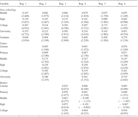
We separate the full sample into the public sector and the private sector employees. The OLS regressions are reported in Tables 4 and 5. The results show that the effects of family background on wages are significant only in the private sector. None of the estimated coef-ficients of family background variables in the public sec-tor are statistically significant (Table 4). In almost all cases, the family background coefficients are smaller in the public than in the private sector sample, so the lack of significance is not due only to the smaller size and larger standard errors of the public-sector sample. The estimated results in the private sector (Table 5) are simi-lar to the results in the full sample (Table 3), with father’s schooling having a larger effect than mother’s schooling. In addition, own education coefficients are greater for the public sector, suggesting that the effect
11Parish and Willis (1993) analyze parental investment in children’s education in Taiwan.
of education is larger in the public sector than in the private sector.12
There are a number of possible explanations for the difference in returns to family background between sec-tors. First, entry into many public sector jobs requires applicants to first pass a civil service exam. Family back-ground may be influential in preparing applicants to pass this hurdle, after which background may have much less influence on wages. In addition, although one might expect variation in wages to be smaller in the public than in the private sector, because of the smaller range of jobs available, such an effect is not reflected in our data. As shown in Table 2, the standard deviation of wages is modestly larger for the public than for the private sec-tor employees.
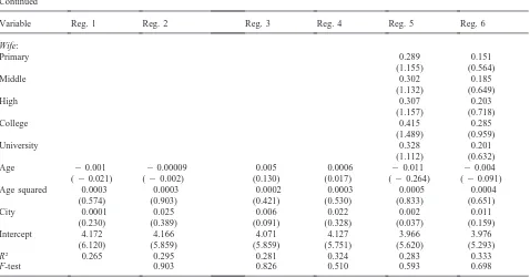
4.2. Effects of wife’s background
We are also interested in the effect of the spouse’s education on workers’ returns to schooling. In addition to the variables discussed above, we add variables for
Table 5
Wage equations estimation in the private-sector sample (OLS). Dependent variable: log of hourly wagea
Variable Reg. 1 Reg. 2 Reg. 3 Reg. 4 Reg. 5 Reg. 6
Own schooling:
Middle 0.107 0.082 0.096 0.079 0.075 0.055
(2.468) (1.875) (2.214) (1.810) (1.730) (1.249)
High 0.159 0.107 0.135 0.101 0.089 0.045
(3.827) (2.467) (3.145) (2.304) (1.983) (0.988)
College 0.287 0.214 0.256 0.207 0.173 0.113
(4.832) (3.441) (4.196) (3.312) (2.681) (1.695)
University 0.355 0.212 0.305 0.216 0.165 0.051
(4.751) (2.596) (3.813) (2.618) (1.882) (0.554)
Graduate 0.660 0.484 0.642 0.494 0.428 0.279
(3.054) (2.188) (2.949) (2.220) (1.926) (1.218)
Father:
Literate 0.095 0.091 0.076
(1.584) (1.472) (1.249)
Primary 0.099 0.087 0.071
(2.540) (2.158) (1.768)
Middle 0.175 0.167 0.147
(2.762) (2.524) (2.269)
High 0.229 0.250 0.218
(2.981) (2.976) (2.634)
College 0.302 0.319 0.261
(2.487) (2.492) (2.059)
University 0.340 0.361 0.319
(3.255) (3.152) (2.843)
Mother:
Literate 0.035 0.006 0.003
(0.673) (0.108) (0.498)
Primary 0.078 0.041 0.040
(2.477) (1.238) (1.251)
Middle 0.023 20.100 20.116
(0.277) (21.115) (21.307)
High 0.072 20.101 20.067
(0.614) (20.802) (20.541)
College 0.256 0.044 0.010
(1.432) (0.233) (0.055)
Continued.
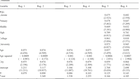
wife’s schooling to the regressions. Note that the omitted category of wife’s schooling is illiterate. Wife’s school-ing plays a significant role in explainschool-ing wages in the full sample and the private sectors, but not in the public sector. Regression 5 of Tables 3 and 5, which include the wife’s education, show that the estimated coefficients of own schooling remain statistically significant and positive while they are smaller than the corresponding coefficients in regression 1. The estimated coefficients on wife’s schooling are statistically significant and posi-tive for all categories. It is interesting to find that the coefficients on wife’s schooling are larger than the corre-sponding coefficients on either parents’ schooling in regressions 2 to 4 of Tables 3 and 5. Inclusion of wife’s schooling also causes a larger reduction in the estimated returns to husband’s post-middle schooling categories
Table 5 Continued
Variable Reg. 1 Reg. 2 Reg. 3 Reg. 4 Reg. 5 Reg. 6
Wife:
Literate 0.675 0.682
(2.523) (2.558)
Primary 0.678 0.647
(5.462) (5.209)
Middle 0.669 0.632
(5.181) (4.900)
High 0.789 0.741
(6.013) (5.640)
College 0.861 0.810
(5.956) (5.571)
University 0.973 0.945
(6.027) (5.836)
Age 0.073 0.074 0.074 0.075 0.057 0.059
(4.456) (4.569) (4.518) (4.569) (3.459) (3.612)
Age squared 20.0009 20.0009 20.001 20.001 20.0006 20.0007
(24.083) (24.172) (24.124) (24.168) (22.831) (22.984)
City 0.075 0.074 0.076 0.079 0.059 0.064
(2.196) (2.176) (2.209) (2.309) (1.771) (1.902)
Intercept 3.211 3.117 3.166 3.108 2.768 2.698
(11.211) (10.837) (11.007) (10.761) (9.436) (9.133)
R2 0.079 0.098 0.086 0.103 0.125 0.143
F-test 3.349 1.538 2.255 8.166 4.105
aNote: t-statistics are in parentheses. Sample sizes are 947. F-test: null hypothesis is that all family background schooling coefficients equal zero.
hire their son-in-law. All three interpretations may con-tribute to the substantial effects of the wife’s schooling in the wage function, but cannot be distinguished using our data.
We include the whole set of family background vari-ables including parents’ and wife’s education in regression 6 of Tables 3–5. In both the full sample and the private sector (Tables 3 and 5), the magnitudes of the coefficients on own schooling are the smallest among the six regressions. Wife’s schooling always has a larger effect than parents’ schooling. The F-test allows us to reject the hypothesis that the coefficients for all family background variables are equal to zero at the 1% level. In the public sector, by contrast, the effects of wife’s schooling are much smaller, but still larger than the effects of the parents’ education (Table 4).13None of the
coefficients are individually significant, however, and the
F-statistic indicates that we cannot reject the null
hypoth-esis that the schooling coefficients for the wife and par-ents are jointly equal to zero.
13The coefficients on wife’s education are larger than the corresponding coefficients on father’s or mother’s education at each level of schooling, except the high school coefficient is larger for the mother than the wife.
4.3. Predicted returns to marginal stages of schooling
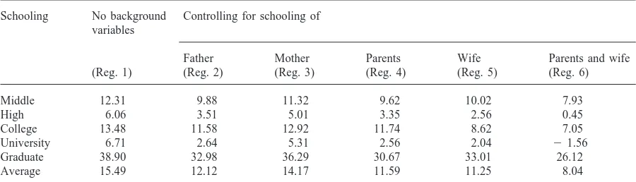
Using the regression results in the full sample (Table 3), the percent change in wages associated with marginal stages of schooling are summarized in Table 6. The table reports the reduction in estimated returns to schooling caused by including alternative sets of family back-ground variables, i.e. the bias caused by omitting family background variables from the wage function. Without including any family background variables (regression 1), the average return to schooling is 15.5%. Adding the schooling of the worker’s wife instead of his father or mother causes a larger decline for high school, college, and university education. Inclusion of the wife’s and par-ents’ schooling jointly causes a substantially larger decrease than either the wife’s or parents’ schooling alone at all levels, with the average return dropping 7.5 percentage points, from 15.5 to 8.0%. Overall, omitting family background variables, especially the wife’s edu-cation, may cause substantial upward bias in the esti-mated returns to schooling for the married male sample.
4.4. Measurement errors
Table 6
Predicted returns to marginal stage of schooling: percentage change in wages (full sample) Schooling No background Controlling for schooling of
variables
Father Mother Parents Wife Parents and wife
(Reg. 1) (Reg. 2) (Reg. 3) (Reg. 4) (Reg. 5) (Reg. 6)
Middle 12.31 9.88 11.32 9.62 10.02 7.93
High 6.06 3.51 5.01 3.35 2.56 0.45
College 13.48 11.58 12.92 11.74 8.62 7.05
University 6.71 2.64 5.31 2.56 2.04 21.56
Graduate 38.90 32.98 36.29 30.67 33.01 26.12
Average 15.49 12.12 14.17 11.59 11.25 8.04
Table 7
Measurement errors bias in wage equation (full sample)a No background Controlling for schooling of variables
Father Mother Parents Wife Parents and wife
(Reg. 1) (Reg. 2) (Reg. 3) (Reg. 4) (Reg. 5) (Reg. 6)
bi 0.0820 0.0737 0.0787 0.0735 0.0582 0.0523
R2 0.1078 0.1237 0.1140 0.1278 0.1457 0.1616
R2
sf 0.1742 0.3322 0.2793 0.3496 0.4505 0.5161
Db 5 bi2b1 20.00083 20.00033 20.00085 20.02376 20.02966
mi 20.01453 20.01796 20.01665 20.01845 20.02183 20.02479
Dmi 20.00034 20.00021 20.00039 20.00092 20.01026
Dmi/Dbi 41.43% 64.81% 45.90% 3.89% 34.61%
aNote:b
iis the estimated returns to schooling in regression i, miis measurement error bias.
are included in the wage function. If schooling is meas-ured with error, this estimate may overstate the upward bias that results from omitting family background in regression 1. From Eq. (5), the measurement error bias (m) is
m5 lbs
12R2 sf
(6)
where l 5 Var(e)/Var(S). Table 7 shows the measure-ment-error bias when different sets of family background variables are included, given the assumed values of 1 and true returns to schooling bs. For this analysis, worker’s
schooling is replaced by a single “years of schooling” variable instead of the educational level dummy vari-ables used in Table 3. As shown in Table 7, a regression of worker’s years of schooling on age, age squared, city, and public-sector dummy variables has R2
sf50.1742.
The rate of return to schoolings 0.082.14If we assume
14We follow Eq. (4) in Heckman and Hotz (1986) to calcu-late the returns to schooling. The conventional approach is to proxy work experience by age minus schooling minus 6. In the regression, we include the worker’s age instead of experience.
that observed schooling is 15% measurement error (l 5 0.15) and true returns to schoolingbs50.08, then from Eq. (6) we can calculate that the measurement bias in regression 1 of Table 7 is20.01453. The incremental measurement error bias from regression 1 to regression 2 (Table 3) is20.00034 compared with a change in the estimate ofbof20.00083. This indicates 41% of the observed change inbwould be explained by the increase in measurement error bias. From the other regressions of Table 3, except regression 5 (for the wife’s education), the measurement errors explain more than 30% of the observed decline in the estimated coefficient. The results in Table 7 suggest that, because of measurement errors, the omitted variable bias when family background is not included in the wage equation is smaller than the 9–48% suggested by Table 6. Lam and Schoeni (1993) also found that measurement error accounts for part of the
apparent omitted variable bias in the Brazilian labor mar-ket. The small measurement error bias in the wife’s edu-cation variable indicates that wife’s background is the most important family background variable in the hus-band’s wage equation.
5. Conclusion
Including family background variables in the wage equation significantly decreases estimated returns to the worker’s own schooling. Using data on the schooling of family members, including the father, mother, and wife, we identify substantial effects of family background on returns to schooling in Taiwan. Our study indicates that the father’s schooling is more important than the mother’s schooling in explaining the variation in work-er’s wages in Taiwan. This result differs from the find-ings of Heckman and Hotz in the case of Panamanian males. In Taiwan, a university-educated father is associa-ted with a 15% wage advantage compared with an illiter-ate father. What stands out as more noteworthy, perhaps, is the dominance of the wife’s schooling over own father’s schooling as an influence on worker’s wages. We note that these results are consistent with high assortative mating in the marriage market in Taiwan.
The effects of family background presented above are shown to apply to the private sector; we fail to see as large an effect in the public sector. The difference may result from greater meritocracy in the public sector, which would limit the effects of family connections on job and wage level (although family background might be influential in obtaining a public sector job). Alterna-tively, the difference may result from greater competi-tiveness in the private sector. The private sector in Tai-wan is very competitive, with little unionisation. If wages in the public sector are less sensitive to pro-ductivity differences and family background is an indi-cator of productivity, we would also expect to see a greater apparent effect of family background on wages in the private sector.
Our analysis suggests that including family back-ground variables may overstate the decline in the returns to schooling because of errors in measured schooling. The measurement bias is estimated to account for 35% of the decline in estimated return to schooling when all family background variables are considered in the wage equation.
Acknowledgements
We thank John Riew, Robert Schoeni, Wim Vijver-berg, and the referees for valuable comments and suggestions.
References
Armitage, J., & Sabot, R. (1987). Socioeconomic background and the returns to schooling in two low-income countries.
Economica, 54, 103–108.
Becker, G.S., & Tomes, N. (1979). An equilibrium theory of the distribution of income and intergenerational mobility.
Journal of Political Economy, 87, 1153–1189.
Behrman, J., & Wolfe, B. (1984). The socioeconomic impact of schooling in a developing country. Review of Economics
and Statistics, 66(2), 296–303.
Benham, L. (1974). Benefits of women’s education within mar-riage. In T.W. Schultz, Economics of the family (pp. 375– 389). Chicago, IL: University of Chicago Press.
Blau, P., & Duncan, O.D. (1967). The American occupational
structure. New York: Wiley.
Carynoy, M. (1967). Earnings and schoolings in Mexico.
Econ-omic Development and Cultural Change, 15, 408–419.
Daniel, K. (1995). The marriage premium. In M. Tommasi, & K. Ierulli, The new economics of human behavior. Cam-bridge: Cambridge University Press.
Dougherty, C., & Jimmenez, E. (1991). The specification of earnings function: tests and implications. Economics of
Edu-cation Review, 10, 85–98.
Fei, J.C.H., Ranis, G., & Kuo, S.W.Y. (1979). Growth with
equity: the Taiwan case. Oxford: Oxford University Press.
Fields, G.S. (1992). Living standards, labor markets and human resources in Taiwan. In G. Ranis, Taiwan: from developing
to mature economy. Boulder, CO: Westview Press Inc.
Griliches, Z. (1977). Estimating the returns to schooling: some econometric problems. Econometrica, 45, 1–22.
Heckman, J.J., & Hotz, V.J. (1986). An investigation of the labor market earnings of Panamanian males: evaluating the sources of inequality. Journal of Human Resources, 23, 507–542.
Hou, J.W. (1993). Wage comparison and job distributional dif-ferences between public and private sectors. Taiwan
Econ-omic Review, 213(3), 249–287.
Hungerford, T., & Solon, G. (1987). Sheepskin effects in the returns to education. Review of Economics and Statistics,
69(1), 175–177.
Lam, D., & Schoeni, R.F. (1993). Effects of family background on earnings and returns to schooling: evidence from Brazil.
Journal of Political Economy, 101(4), 710–740.
Lam, D., & Schoeni, R.F. (1994). Family ties and labor markets in the United States and Brazil. Journal of Human
Resources, 29, 1235–1258.
Ozdural, S. (1993). Intergenerational mobility: a comparative study between Turkey and the United States. Economics
Letters, 43, 221–230.
Parish, W.L., & Willis, R.J. (1993). Daughters, education, and family budgets: Taiwan experiences. Journal of Human
Resources, 28(4), 863–898.
Psacharopoulos, G. (1985). Returns to education: a further inter-national update and implications. Journal of Human
Resources, 20(4), 583–604.
Sahn, D., & Alderman, H. (1988). The effects of human capital on wages, and the determinants of labor supply in developing countries. Journal of Development Economics,
29(2), 157–183.
Srinivasan, Handbook of development economics (pp. 543– 630). Amsterdam: North Holland.
Stelcner, M., Arriagada, A.M., & Moock, P. (1987). Wage determinants and schooling attainment among men in Peru. Living studies measurement study working paper no. 38. Washington, DC: World Bank.
Strauss, J., & Thomas, D. (1994). Wages, schooling and back-ground: investments in men and women in urban Brazil. In N. Birdsall, B. Bruns, & R. Sabot, Opportunity foregone:
education, growth and inequality in Brazil. Washington,
DC: World Bank.
Strauss, J., & Thomas, D. (1995). Human resources: empirical modeling of household and family decisions. In J. Behrman,
T.N. Srinivasan, Handbook of development economics (Vol. 3A, pp. 1883–2023). Amsterdam: North Holland. Thomas, D. (1990). Intra-household resource allocation: an
inferential approach. Journal of Human Resources, 25(4), 635–664.
Van Der Gaag, J., & Vijverberg, W. (1989). Wage determinants in Cote D’Ivoire: experience, credentials, and human capi-tal. Economic Development and Cultural Change, 37, 371–381.