Testing for stationarity-ergodicity and for
comovements between nonlinear discrete time
Markov processes
Valentina Corradi
!
, Norman R. Swanson
"
, Halbert White
#
,
*
!University of Pennsylvania, Philadelphia, PA 19104, USA "Pennsylvania State University, University Park, PA 16802, USA
#University of California-San Diego, Department of Economics, 9500 Gilman Driver, La Jolla CA 92093-0508, USA
Abstract
In this paper we introduce a class of nonlinear data generating processes (DGPs) that
are"rst order Markov and can be represented as the sum of a linear plus a bounded
nonlinear component. We use the concepts of geometric ergodicity and of linear stochas-tic comovement, which correspond to the linear concepts of integratedness and cointeg-ratedness, to characterize the DGPs. We show that the stationarity test due to Kwiatowski et al. (1992, Journal of Econometrics, 54, 159}178) and the cointegration test of Shin (1994, Econometric Theory, 10, 91}115) are applicable in the current context, although the Shin test has a di!erent limiting distribution. We also propose a consistent test which has a null of linear cointegration (comovement), and an alternative of &non-linear cointegration'. Monte Carlo evidence is presented which suggests that the test has useful"nite sample power against a variety of nonlinear alternatives. An empirical illustration is also provided. ( 2000 Elsevier Science S.A. All rights reserved.
JEL classixcation: C12; C22
Keywords: Cointegration; Linear stochastic comovement; Markov processes; Nonlin-earities
*Corresponding author. Fax: (858)-534-7040. E-mail address:[email protected] (H. White)
1. Introduction
In most econometric applications there is little theoretical justi"cation for believing in the correctness of linear speci"cations when modeling economic variables. In consequence, nonlinear time series models have received increasing attention during the last few years (for example, see Tong (1990), Granger and TeraKsvirta (1993), Granger (1995), Granger et al. (1997), Anderson and Vahid (1998), and the references contained therein). Nevertheless, when nonlinear models are speci"ed, correct inference requires some knowledge as to whether the underlying data generating processes (DGPs) are stationary and ergodic in some appropriate sense, or instead have trajectories that explode with positive probability as the time span approaches in"nity. In the linear case it is common to test for unit roots in order to check whether a series is integrated of order 1, denotedI(1), or integrated of order 0, denotedI(0), where a process is said to be
I(d) if the scaled partial sum of its dth di!erence satis"es a functional central limit theorem (FCLT). If one has two or moreI(1) series, it is common to test for cointegration in order to determine whether there exists a linear combination of the variables which isI(0). However, the concepts of integratedness and cointeg-ratedness typically apply to linear DGPs, in the sense that the conditional mean is assumed to be a linear function of a set of conditioning variables. In contrast, strictly convex or concave transformations of random walks have a unit root component, but they are notI(1), in the sense that their"rst di!erences need not be short memory processes (Corradi, 1995).
In this paper we examine nonlinear DGPs that are"rst-order Markov and can be represented as the sum of a linear plus a bounded nonlinear component. For such DGPs, we exploit results by Chan (see Appendix to Tong, 1990) to obtain simple conditions for distinguishing between processes that are geomet-ric ergodic (and thus strong mixing) and processes having trajectories that explode with positive probability as¹PR. Using these conditions, we replace the concept of cointegratedness with concept of linear stochastic comovement. Speci"cally, ifX"(X
i,t,i"1, 2,2,p,t"1, 2,2,¹) is a nonergodic Markov
process inRp, in the sense that the trajectories explode with positive probability as¹PR, but there exists anrdimensional linear combination, sayh@0X
t, with h0a full column rankp]rmatrix (r(p) that is ergodic inRr, then there islinear stochastic comovementamong the components ofX. We use the term&Markov process'to mean a process in which the state space is continuous and time is discrete. Note that our approach di!ers from that of Granger and Hallman (1991). According to their terminology, two long memory series, say X
t and >
thave anattractorif there exists a linear combination of nonlinear functions of X
tand>t, sayg(Xt)!h(>t) that is short memory. In contrast, we consider the
hypothesis of no unit root can be formulated in the same way. Similarly, the null hypothesis of linear stochastic comovement and the null hypothesis of cointeg-ration can be formulated in the same way. Thus, the presence of stochastic comovement implies the presence of cointegration among the linear compo-nents of our nonlinear models, and vice versa. Given this framework, one of our main goals is to propose a &nonlinear cointegration' test, for which the null hypothesis is linear cointegration, and the alternative is nonlinear cointegration. The test which we propose is consistent against a wide variety of nonlinear alternative, including neural network models with sigmoidal activation func-tions (e.g. logistic cumulative distribution funcfunc-tions (cdfs)). We show using a series of Monte Carlo experiments that our nonlinearity test has the ability to distinguish between a variety of linear and nonlinear models for moderate sample sizes.
As we typically do not have information concerning the precise form of the nonlinear component, we examine the e!ect that neglected nonlinearities have on tests for the null of stationarity (unit root) and for the null of cointegration (no cointegration). We note that in the presence of neglected nonlinearities, tests with a null hypothesis of integratedness, as well as tests with a null hypothesis of no cointegration, do not have easily determined limiting distributions. This is because in the presence of neglected non-linearities the innovation terms are no longer strong mixing and in general do not satisfy standard invariance prin-ciples. Consequently, standard unit root asymptotics no longer necessarily apply. Along these lines, we "rst examine the stationarity test proposed by Kwiatkowski et al. (1992). We show that this test has a well-de"ned limiting distribution under the null hypothesis of general nonlinear stationary-ergodic DGPs and has power not only against the alternative of integratedness, but also against alternatives involving a range of nonlinear-nonergodic processes. Sec-ond, we show that the Shin (1994) test for the null hypothesis of cointegration can be used to test for stochastic comovement, although the limiting distribution of the test is di!erent. Interestingly, the ADF unit root and Johansen cointegra-tion tests no longer have straightforward limiting distribucointegra-tions in general. Nevertheless, we show using a series of Monte Carlo experiments that these tests may still be reliable in practice, in the sense that they exhibit moderate bias and reasonable power (e.g. the empirical power is more than 0.5 for samples as small as 250 observations when the nonlinear component in our model is a logistic cdf ). The rest of the paper is organized as follows. In Section 2 we describe our set-up. In Section 3, we examine stationary-ergodicity and cointegration (comovement) tests. In Section 4 we propose a test for distinguishing between linear and nonlinear cointegration. In Section 5 we summarize the results from a series of Monte Carlo experiments, while Section 6 contains an empirical illustration. Section 7 concludes. All the proofs are collected in an Appendix. In the sequel,Ndenotes weak convergence;=denotes a standard Brownian
2. Assumption and preliminary results
We start by considering the following DGP:
X
t"AXt~1#g0(h10@Xt~1,2,hj@0Xt~1)#et, (2.1)
where X
t:XPRp, t"1, 2,2,¹ with (X,F,P) an underlying probability
space, andhi0denotes theith-column ofh0, a full column rankp]rmatrix, with
r)p, and 1)j)r(p. Assume also that A1.e
tis identically and independently distributed (iid), has a distribution which
is absolutely continuous with respect to the Lebesgue measure inRp, and has positive density everywhere.
A2. E(et)"0 and E(ete@t)"RwhereRis positive de"nite and E((e@tet)2)(R. A3.g
0: RjPRp is bounded, Lipschitz continous, and di!erentiable in the
neighborhood of the origin. Furthermore,g
0 is not everywhere equal to
zero.
Although A3 is a somewhat strong assumption, it should be noted that a wide variety of nonlinearities are contained within the class of DGPs which we examine. For example various neural network models with sigmoidal activation functions satisfy A3. Examples include feedforward arti"cial neural networks with a single &hidden unit' and either logistic or normal cdfs as activation functions (see, e.g. Kuan and White, 1994). Other examples of functional forms forg
0include modi"ed exponential autoregressive models whereg0(x)"xe~x 2
(Tong, 1990, p. 129), and symmetric smooth transition autoregressive (STAR) type models where g0(x)"x/(1#ex2
). On the other hand, the logistic STAR
g
0(x)"x/(1#e~x) and the exponential STAR (g0(x)"x(1!ex2)) (see, e.g.
TeraKsvirta and Anderson, 1992) are ruled out. Furthermore g
0 may contain
a constant term. Higher-order lag structures are allowed by a variant of (2.1), as ap-dimensional k-order Markov process can be written as a kp-dimensional
"rst-order Markov process with a positive semi-de"niteRof rankp.
Proposition 2.1. For DGP (2.1), suppose that A1}A3 hold. If all of the eigenvalues of the matrix A are strictly less than one in absolute value, then X"(X
i,t; i"1,2,p,t"1, 2,2,¹)is a geometric ergodic Markovprocess inRp,with an
invariant probability measure which is absolutely continuous with respect to the Lebesgue measure inRp.
Dexnition 2.2. (Linear stochastic comovement). Assume that Xis a nonergodic Markov process in Rp, in the sense that each component of X approaches in"nity with positive probability as¹PR. Assume also that there exists some full column rank p]r (r(p) matrix, h0"(h10,2,hr0), such that h@0Xt is an
Rr. Then, there existslinear stochastic comovementamong the components ofX, andhi0is theithcomovementvector,i"1,2,r.
In the sequel we specialize De"nition 2.2. to the DGP given in (2.1). For this reason, we useh0in (2.1). Now letU,A!I, whereIis thep]pidentity matrix. We assume either of the following:
A4(i). U"ah@
0, whereaandh0are full column rankp]rmatrices,r(p. The
eigenvalues ofU, sayji, are such that!2(j
1)j22)jr(0.
A4(ii). A"I.
Proposition 2.3. Assume that (2.1), and A1}A4(i) hold.Then: (i)X is a nonergodic Markovprocess in RpandP(EX
TEPR),g'0as¹PR.
(ii) h@0X
t is a geometric ergodic Markovprocess inRrwhich has an invariant
probability measure,n,that is absolutely continuous with respect to the Lebesgue measure(k)inRr, and which has densityl"dn/dk.Further,
h@0*X
t"h@0UXt~1#h@0g0(h10@Xt~1,2,hj@0Xt~1)#h@0et.
It follows that there is stochastic comovement among the components of
X(from De"nition 2.2).
Proposition 2.4. Assume that (2.1), A1}A3, and A4(ii) hold. Then both X andh@0X
are nonergodic Markovprocesses inRpandRr,respectively. It also follows that
P[EX
TEPR]'0 and P[Eh@0XTEPR]'0.
The ergodicity of the process de"ned in (2.1) is implied by the stability of the associated deterministic dynamical system. This allows us to analyze the er-godicity of the stochastic system by examining the eigenvalues ofAorU. This means that the same conditions which ensure the ergodicity of the linear part of our model also ensure the ergodicity of the entire nonlinear process. Thus, for the processes which we are considering, the existence of stochastic comovement is equivalent to the existence of cointegration among the linear components in the model. In particular, the existence of r comovement vectors implies the existence ofrcointegrating vectors in the linear part of the model. For brevity, we refer to this subsequently as just&cointegration'.
Observe that in the case whereA!I"U"ah@
0there is a clear interpretation
of the argument ofg
0in terms of cointegrating vectors. On the other hand when A"I,g
0depends on some generic linear combination of theX's. Thus under
keep a &continuous' relationship between the arguments of g
0and A!I, we
could consider the following variation of (2.1):
*X
t"ah@0Xt~1#g0((h0, 0)@Xt~1)#et,
whereh0is ap]r(r(p) matrix, 0 is ap](p!r) matrix of zeroes, andh0"0 whenr"0. Thus, whenr"0,X
tis an I(1) process with a deterministic trend
component. It should be noted that all the theorems below hold for this special case. (This point was kindly communicated to us by Herman Bierens.)
The following facts will be frequently used in the paper.
Fact 2.5 (From Athreya and Pantula, 1986, Theorem 1). Geometric ergodic discrete time Markovprocesses are strong mixing. Further, the speed at which the mixing coezcient declines to zero is proportional to the speed at which the transition distribution converges to the invariant probability measure. Thus, when the transition distribution approaches the invariant probability measure at a geo-metric rate, the mixing coezcients also decay at a geometric rate.
To ensure the next fact, we add another assumption. A5.X
0is a randomp-vector andh@0X0is drawn from a densityl, wherelis the
density associated with the invariant probability measure,n, as de"ned in Proposition 2.3(ii).
Fact 2.6 (from Meyn, 1989). For (2.1), if A1}A4(i) and A5 hold, then h@0X thas
density lfor allt"1, 2,2,¹. Thus X is strictly stationary, in addition to being
a geometric ergodic process (and thus strong mixing).
3. Testing for stationarity}ergodicity and for linear stochastic comovement
We begin by considering the one-dimensional case, (i.e.p"1), and the test proposed by Kwiatkowski et al. (1992). Without loss of generality assume that
h0"1, so that (2.1) can be written as:
X
t"aXt~1#g0(Xt~1)#et (3.1)
The null hypothesis considered by Kwiatkowski et al. (1992) is rather general and includes (3.1) when a(1, and A5 holds. However, the alternative is somewhat restrictive, asX
tis assumed to be an integrated time series
character-ized by the sum of a random walk component, a stationary (short memory) component, and possibly a time trend component. This alternative does not include nonlinear nonergodic DGPs such as (3.1), witha"1. For this case the
"rst di!erence ofX
tis not a strong mixing process, in general, as it displays&too
Theorem 3.1. Assume that (3.1), and A1}A3 hold.
(i) IfDaD(1,and A5 holds, then
S T"
1
s2 lT
1
¹2 T + t/1
A
t + j/1
(X j!XM )
B
2 N
P
10
<2
r dr,
where<
r"=r!r=1,=r"W(r),0)r)1,XM "¹~1+Tt/1Xt,and s2lT"1
¹ T + t/1
(X
t!XM )2#
2
¹ lT
+ t/1
lT
+ j/1
A
1! t l
T#1
B
] +T j/t`1
(X
j!XM )(Xj~t!XM ),
withl
T"o(¹1@2).
(ii) Ifa"1,then
P[S
T'CT]P1 as¹PR,
whereC
TPRand
C TlT
¹ P0,as ¹PR.
Part (i) of Theorem 3.1 ensures that the distribution under our null is exactly the same as the distribution of the Kwiatkowski et al. (1992) test statistic. Further, part (ii) of Theorem 3.1 ensures that under our alternative,S
Tdiverges
at the same rate as does the Kwiatkowski et al. (1992) statistic under their alternative. However, note that our alternative is more general than their alternative of integratedness, as it includes DGPs consisting of a unit root component plus a possibly long memory component. Assumption A5, which ensures strict stationarity, can be relaxed and replaced by the weaker property of constancy of the"rst moment (i.e. E(X
t)"E(X) for allt). If E(Xt) depends ont,
though, the partial sums ofX
t!XM do not necessarily satisfy a FCLT and so the
numerator of the test statistic may diverge. Recently, Domowitz and El-Gamal (1993,1997) have proposed a test for the null hypothesis of ergodicity. Their test is based on the convergence of Cesaro averages of the iterates from di!erent initial densities, has the correct size under the null, regardless of whether the process is stationary or not, and has power against the alternative of noner-godicity given a maintained assumption of stationarity.
to the existence of cointegration, in the current context. Thus, tests that have (no) stochastic comovement under the null hypothesis are equivalent to tests that have (no) cointegration under the null. In this section we consider the following two DGPs:
*X
t"g0(h@0Xt~1)#et (3.2)
and
*X
t"UXt~1#g0(h@0Xt~1)#et, (3.3)
where h0"(!h
1,h2)@ and U"ah@0, such that !2(!a1h1#a2h2(0.
From (3.3) we have that
h@0*X
t"(!a1h1#a2h2)h@0Xt~1#h@0g0(h@0Xt~1)#h@0et. (3.4)
Let
h~12 h@0"c@
0"(!h~12 h1, 1)"(!b0, 1)
and
d"!a
1h1#a2h2,
so that
c@0*Xt"dc@
0Xt~1#c@0g0(h@0Xt~1)#c@0et. (3.5)
Ash@0X
tis a geometric ergodic process,c@0Xtis also a geometric ergodic process.
It is convenient to use a triangular representation of (3.3):
X 1,t"
t + j/1
l1,
j and X2,t"b0X1,t#l2,t, (3.6)
where
l1,t"a
1h2c@0Xt~1#g0,1(h@0Xt~1)#e1,t, (3.7) l2,
t"(d#1)c@0Xt~1#c@0g0(h@0Xt~1)#c@0et, (3.8)
andg
0,i,i"1, 2, denotes the ith component ofg0.
In order to test the null hypothesis of stochastic comovement, we use the statistic proposed by Shin (1994) for testing the null of cointegration. Although stochastic comovement and cointegration are equivalent concepts, we show that, unless E(l1,
t)"0 for allt, the distribution that we obtain under our null
unless E(l1,t)"0,X
1,tdisplays a deterministic trend component. In fact, we can
writeX
1,tin (3.6) as X1,
t"nt#+t j/1
(l1,j!n), where E(l1,
t)"n for allt, as under A5, l1t is strictly stationary. X2,t can be
written in an analogous way. The role of the comovement vector is to&cancel out' both stochastic and deterministic trends when the linear combination,
X
2,t!b0X1,t, is formed. Furthermore,X2,t!b0X1,tis an ergodic process. As X
1,t is dominated by its trend component, the estimator of the comovement
vector is ¹3@2-consistent. Also, the asymptotic distribution of ¹3@2(bKT!b 0),
wherebKTis the coe$cient from the regression of X
2,t onX1,tand a constant
term (as in (3.6)), di!ers from the asymptotic distribution for the driftless case. Note that the only di!erence between X
2,t in (3.6) and Eq. (2.1) in Hansen
(1992a) is that E(l2,t)"/O0, so that we need to introduce a constant term into our cointegrating regression.
Theorem 3.2. Assume that (3.3), and A1}A4(i), A5 hold, and thatE(l1,
t)O0.Then ¹3@2(bKT!b
0)N
12
n pl2
AP
10 sd=
s!1/2=1
B
,wherep2l2"<ar(l
2,t), as dexned in (3.8), and=s"W(s),0)s)1.
As in Theorem 3.1(i), we require only that the"rst moment ofX
tis constant,
and A5 ensures this. The same is also true for Theorem 3.3(i) below. Note that:10sd=
s!1/2=1"1/2=1!:01=sds&N(0, 1/12), as:10=sds&
N(0, 1/13) and Cov(1/2=
1, :10=sds"1/4. Thus, the limiting distribution in
Theorem 3.2 is normal. The representation of the limiting distribution given in Theorem 3.2 is more convenient for computing the limiting distribution of the test for the null of stochastic comovement (cointegration). If instead E(l1,
t)"0
for allt, then
¹(bKT!b 0)N
AP
1
0
=2
1,sds
B
~1AP
10 =
1,sd=2,s
B
#*12,where*12"0 and E(=
1,t,=2,t)"0 for allt, only if E(l1,t,l2,s)"0 for allt,s.
nonlinear component, in general, does not satisfy a standard invariance prin-ciple.)
We now show that the Shin (1994, Eq. (6))C
ktest can be applied to test the
null hypothesis of stochastic comovement, although the limiting distribution under the null is di!erent. LetmKtbe the residual from the regression ofX
2,ton X
1,tand a constant term.
Theorem 3.3. (i) Assume that (3.3), and A1}A4(i), A5 hold, and that E(l1,
(ii) Assume that (3.2), and A1}A3, A4(ii) hold. Then,
P
C
1From part (i) of Theorem 3.3 note that the asymptotic distribution under the null is a functional of only one Brownian motion=, where=is the weak limit,
property rescaled, of the partial sums of l2,
t!E(l2,t)"c@0Xt!E(c@0Xt). Thus,
the asymptotic behavior of the statistic is not a!ected by whetherl1,
tandl2,tin
(3.7) and (3.8) are correlated or not. As mentioned above, this is due to the fact that the asymptotic behavior ofX
1,tis dominated by its trend component. This
di!ers from the linear case,g0"0, in which the non-zero correlation between
Linear stochastic comovement test critical values Nominal size
1% 5% 10% 90% 95% 99%
0.219 0.150 0.121 0.028 0.023 0.018
Note that our critical values are smaller than those reported in Shin (1994) for his
Cktest statistic. This di!erence arises because of the nonlinear component in (3.3). In practice we do not know whether E(l1,t)"0 or not. If E(l1,t)O0, then the critical values tabulated above should be used. On the other hand, if E(l1,t)"0, then the asymptotic distribution of our test is the same as that ofC
kin Shin (1994,
Theorem 1), provided E(l1,tl2,t)"0. Given these facts, we suggest applying the comovement test in the following way. If the test statistic is less than our critical value, accept the null of (cointegration) comovement. On the other hand if the test statistic is above Shin's critical value forCk, we have evidence of the absence of cointegration (comovement). If the test statistic falls in the region between the two critical values (say the &intermediate region'), construct the following statistic:
d
T"¹~1@2+Tt/1p(~1T *X1,t, where p(2T is a consistent estimator of the long run
variance of¹~1@2+*X
1,t. Under cointegration (comovement),dTNN(0, 1) when
E(l1,
t)"0, and diverges at rate¹1@2when E(l1,t)O0. On the other hand, when
there is no cointegration (comovement), we must distinguish between three cases. First, assume that E(l1,t)"0 . Here, there are two cases: (i) E(l1,t)"0 because there is no nonlinear component; or (ii) E(l1,t)"0 because there is zero mean nonlinear component. Under (i),d
Tis normally distributed (asl1,tis a zero mean
mixing process). Under (ii), the statistic is not normally distributed in general. Finally, assume that E(l1,t)O0. In this case, the estimator of the variance term in
d
Tdiverges at a rate less than or equal tol1@2T , while the numerator ofdTdiverges
at a faster rate. These facts suggest a procedure for testing for cointegration (comovement) when the test statistic is in the&intermediate region'. In particular, if we reject E(l1,
t)"0, reject the null of cointegration (comovement). If we fail to
reject E(l1,
t)"0, then use Shin's critical values. (In order to use Shin's critical
values in this case, an e$cient estimator of the cointegrating vector should be constructed, as in Shin (1994).) Note that the use ofd
1may result in the false
rejection of E(l1,
t)"0 when there is no cointegration (comovement) and the
nonlinear component has zero mean. However, in this case we still reject the null of cointegration (comovement), which is the correct inference.
4. Testing for nonlinear cointegration
A number of papers which examine nonlinear cointegration have recently appeared. For example, Balke and Fomby (1997) propose a test for threshold cointegration. Also, Granger (1995) suggests testing for the null of linear cointeg-ration by regressing the residuals from a standard cointegrating regression on their lagged values and a nonlinear function, and then performing a Lagrange Multiplier (LM) type test. A similar approach is examined by Swanson (1999) who regresses the "rst di!erences of the data on their lagged values and on a polynomial function of the cointegrating vector. He shows, using Monte Carlo experiments, that such tests have good power wheng
0is a logistic cdf.
Neverthe-less, this class of tests does not have unit asymptotic power against general nonlinear alternatives. One reason for this is the LM tests are implemented using polynomial test functions, and the use of polynomials does not ensure test consistency.
In our test, cointegration is maintained under both the null and the alterna-tive hypothesis. Let g(
t be the residual andtK be the slope coe$cient from the
least squares regression ofc(@
TXtonc(@TXt~1and a constant, wherec(@T"(!bKT, 1)
tis uncorrelated with any function ofc@0Xt~1. Under the alternative of
nonlinearity of the type described in Section 2,J¹(tKT!t
t includes the neglected nonlinear term
(g
0(h@0Xt~1)!E(g0(h@0Xt~1))), whereh~12 h@0,c@0"(!h~12 h1, 1). Thus,gtis
cor-related with some function ofc@0X
t~1. If we use as a test function, call itg, an
exponential, as in Bierens (1990), or any other generically comprehensive test function, as described in Stinchcombe and White (1998, Section 3, hereafter SW), then under the alternative
E(gt(g
for allq3T, a subset ofRwhose complementT#has Lebesgue measure zero and is not dense inR. Given theJ¹consistency oftKTand the¹3@2consistency ofbKTunder the alternative, we also have
1
¹ T +
q/1
A
g(t
A
g(c(@TXt~1q)!1
¹ T +
q/1 g(c(@
TXt~1q)
BB
PMq in Prob.whereMqO0, for allq3T.
According to Theorem 3.10 in Stinchcombe and White (1998), ifgis a real analytic function, thengdelivers a consistent test, regardless ofg
0, provided that g is not a polynomial. One natural choice for gis the logistic cdf, as it is a non-polynomial real analytic function.
As the parameterqis not identi"ed under the null hypothesis, our tests falls into the class of tests with nuisance parameters present only under the alterna-tive. Thus, although the asymptotic size of the test statistic is not a!ected by the actual value ofq, the"nite sample size will be a!ected, while the power will be a!ected both in"nite samples and asymptotically. Consider the following two DGPs:
*X
t"UXt~1#et (4.3)
and
*X
t"UXt~1#g0(h@0Xt~1)#et, (4.4)
whereh0"h
2c0. Assume thatUsatis"es A4(i),g0satis"es A3, andetsatis"es A1
and A2. From (4.3) note that
*c@0X
t"dc@0Xt~1#c@0et,
and from (4.4) note that
*c@0X
t"dc@0Xt~1#c@0g0(h@0Xt~1)#c@0et,
whered"!a
1h1#a2h2. The proposed test is based on the statistic:
1
J¹ T + t/2
(g(c(@
TXt~1q)!g(6)g(t, (4.5)
whereg(6"(1/¹)+Tt/2g(c(@
TXt~1q). It is shown in the proof of Theorem 4.1 that
(4.5) can be written as 1
J¹ 0 + t/2
((g(c@
TXt~1q)!g6)!M~1(c@
where M (c@
0X)2"E((c@0Xt!c@0XM )2), Mc@0Xg"E((c@0Xt!c@0XM )(g(c@0Xt~1q)g6)),
g6"(1/¹)+Tt/2g(c@0X
t~1q): From the central limit theorem for strong mixing
processes (e.g. White, 1984, p. 124) and the asymptotic equivalence lemma, note that the limiting distribution of (4.6), when scaled byp2
Tis a zero mean normal,
where
A6. The test functiongis a real nonpolynomial analytic function, with bounded
"rst two derivatives.
Note that various sigmoidal functions (e.g. the logistic cdf) satisfy A6.
(ii) For DGP (4.4), suppose that A1}A4(ii), A5}A6 hold, and that g 0 is not
a constant. Then for eachq3T,
P[Dmq
TD2'CT]P1 as¹PR,
whereC
TPRandCTlT/¹P0,as ¹PR.
Note that strict stationarity is required only under the alternative, as the"rst moment of (4.3) is constant. In fact, in Theorem 4.1(ii), as in Theorems 3.1(i), 3.2 and 3.3(i) above, we impose A5 simply because it implies the constancy of the
"rst moment. Also, note that the case whereg
0is constant is covered by the null
hypothesis.
In the current context we do not provide a &sup' type result, as in Bierens (1990) and Stinchcombe and White (1998), for example. The intuitive reason for this is that the o
p(1) term in (4.6) holds pointwise in q, but not necessarily
uniformly inq. As will become clear in the proof of Theorem 5.1, this is due to the fact that in the nonstationary case, we cannot invoke the usual uniform law of large numbers. We appeal instead to invariance principles and to results on convergence to stochastic integrals that hold pointwise inq, but not necessarily uniformly.
As mentioned above, although the asymptotic size of the test statistic is not a!ected by the choice of a particularq, the "nite sample size and power are a!ected. There are at least two ways of addressing this issue. First, we can construct the statistic for di!erentq's and apply Bonferroni type bounds as in Lee et al. (1993), for example. Second, let q1,2,qp be chosen according to
a particular design (e.g. randomly), and let GK be a consistent estimator of Cov(/qi
l,/qlk), so thatGK is the matrix whosei, kelement is given by
1
¹ T + t/1
/Kqi
t/Kqtk#
2
¹ lT
+ t/1
A
1! t l
T#1
B
T + j/t`1/Kqi
j/Kqjk~t,
where/Kqtis de"ned in (4.9), and/q
tis de"ned as in (4.9), but withc(@Treplaced with c@0. Then, (mq1
T,2,mqTp)@GK~1(mqT1,2,mqTp)Ns2p, for arbitrary and"nitep. Whether
the above result also holds forp"p
T, withpTPRat an appropriate rate as ¹PR, is left for future research.
5. Monte Carlo results
In this section, a summary of Monte Carlo experiments based on the above test, and for samples of 100, 250, and 500 observations, is given. For the sake of brevity, much of the discussion focuses on the nonlinear cointegration (NLCI) test.
nonlinearities. As noted above, however, it turns out that the Kwiatkowski et al. (1992) stationarity and the Shin (1994) cointegration tests have well-de"ned limiting distributions and unit asymptotic power, in our context. The same cannot be said for the augmented Dickey}Fuller (ADF) unit root test. In particular, note that under the null hypothesis of a unit root, if we neglect to account for the nonlinear component, the error term is given byl
t"et#g0()),
whereg
0()) is generally not a strong mixing process. Thus, standard unit root
asymptotics no longer apply, and the usual limiting distribution of the ADF test statistic is typically no longer valid (see, e.g. Ermini and Granger, 1993). On the other hand, under the alternative of no unit root, the error term is a strong mixing process, so that we expect ADF tests to have reasonable power in large samples.
Table 1 reports the results from a Monte Carlo experiment based on the ADF test, using data generated according to
X
t"a#bXt~1#cg0(Xt~1)#et,
whereX
tis a scalar,etis a scalar IN(0, 1) random variable,g0()) is the logistic
cdf, anda"0 (results foraO0 and for di!erentg
0()) are qualitatively similar,
and are available upon request from the authors). Notice that in the table,
b varies from !0.9 to 1.0, so that empirical power of a variety of di!erent parameterizations, and empirical size (b"1) is reported. Also, note that the parameterc is alternately!0.5,!0.1, 0.1, and 0.5. Here and below, results based on 5% nominal size tests are reported (results for 10% size tests are similar, and are not included for the sake of brevity). The"nite sample power of the ADF test is good (power is always close to or equal to unity, except when
DbD"0.9), as expected. The"nite sample size of the ADF test is between 0.084 and 0.056, even for samples of 100 observations, and improves as we move from 100 to 500 observations, whenq(
qis used. This suggests that within our context,
the ADF test can still be used to signal the presence of a unit root, even when a bounded nonlinear component is added to the DGP, as long asq(qis used. This is perhaps not surprising, as the mean ofg
0()) is not generally zero. In summary,
one might argue in favour of usingq(qin our context, as the"nite sample size is closer to the nominal size than whenq( andq(kare used. Further, the"nite sample power of theq(qtest is comparable to the power associated with the use ofq( and
q(k, except when b"0.9.
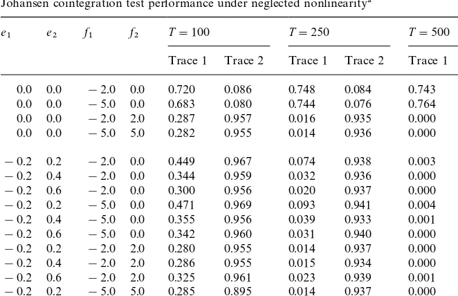
Table 2 reports the results from a Monte Carlo experiment based on the Johansen cointegration test, using data generated according to
*X
t"d#eZt~1#fg0(Zt~1)#et, (5.1)
whereX
t"(X1,t,X2,t)@is a 2]1 vector,etis a 2]1 vector whose components
are distributed IN(0,1),Z
t"!X2,tife1"e2"0, otherwiseZt"X1,t!X2,t, g
Augmented Dickey}Fuller test performance under neglected nonlinearity!
b c T"100 T"250 T"500
q( q(
k q(q q( q(k q(q q( q(k q(q
1.0 !0.5 0.056 0.086 0.084 0.054 0.103 0.086 0.050 0.115 0.098
1.0 !0.1 0.089 0.067 0.071 0.109 0.061 0.061 0.121 0.066 0.067
1.0 !0.5 0.016 0.053 0.067 0.009 0.032 0.057 0.003 0.027 0.054
1.0 !0.5 0.001 0.015 0.067 0.000 0.006 0.056 0.000 0.005 0.057
!0.9 !0.5 1.000 1.000 1.000 1.000 1.000 1.000 1.000 1.000 1.000
!0.6 !0.5 1.000 1.000 1.000 1.000 1.000 1.000 1.000 1.000 1.000
!0.3 !0.5 1.000 1.000 1.000 1.000 1.000 1.000 1.000 1.000 1.000
0.3 !0.5 1.000 0.999 0.996 1.000 1.000 1.000 1.000 1.000 1.000
0.6 !0.5 0.996 0.994 0.985 1.000 1.000 1.000 1.000 1.000 1.000
0.9 !0.5 0.737 0.727 0.529 0.998 0.999 0.994 1.000 1.000 1.000
!0.9 !0.1 1.000 1.000 1.000 1.000 1.000 1.000 1.000 1.000 1.000
!0.6 !0.1 1.000 1.000 1.000 1.000 1.000 1.000 1.000 1.000 1.000
!0.3 !0.1 1.000 1.000 0.999 1.000 1.000 1.000 1.000 1.000 1.000
0.3 !0.1 1.000 0.999 0.995 1.000 1.000 1.000 1.000 1.000 1.000
0.6 !0.1 0.999 0.989 0.979 1.000 1.000 1.000 1.000 1.000 1.000
0.9 !0.1 0.821 0.443 0.286 1.000 0.983 0.912 1.000 1.000 1.000
!0.9 0.1 1.000 1.000 1.000 1.000 1.000 1.000 1.000 1.000 1.000
!0.6 0.1 1.000 1.000 1.000 1.000 1.000 1.000 1.000 1.000 1.000
!0.3 0.1 1.000 1.000 0.999 1.000 1.000 1.000 1.000 1.000 1.000
0.3 0.1 1.000 0.999 0.993 1.000 1.000 1.000 1.000 1.000 1.000
0.6 0.1 1.000 0.985 0.973 1.000 1.000 1.000 1.000 1.000 1.000
0.9 0.1 0.633 0.286 0.185 0.997 0.906 0.712 1.000 1.000 0.997
!0.9 0.5 1.000 1.000 1.000 1.000 1.000 1.000 1.000 1.000 1.000
!0.6 0.5 1.000 1.000 1.000 1.000 1.000 1.000 1.000 1.000 1.000
!0.3 0.5 1.000 1.000 0.999 1.000 1.000 1.000 1.000 1.000 1.000
0.3 0.5 0.999 0.998 0.990 1.000 1.000 1.000 1.000 1.000 1.000
0.6 0.5 0.972 0.973 0.948 1.000 1.000 1.000 1.000 1.000 1.000
0.9 0.5 0.022 0.280 0.184 0.080 0.783 0.606 0.690 0.995 0.978
!Based on the augmented Dickey}Fuller (ADF) test, entries correspond to the empirical frequency of rejection of the null hypothesis of a unit root. Three versions of the test regressions are run: with no constant or linear deterministic trend (q(), with a constant only (q(k), and with a constant and a linear determinisitic trend (q(
q). Data are generated according to the following process:Xt"a#bXt~1#cg0(Xt~1)#et, whereXtis a scalar,etis a scalar IN(0, 1)
random variable,g
0()) is the logistic cdf, anda"0.0. The"rst four rows of entries in the table report the empirical size of the test based on a 5% nominal
size, while the remaining rows report the empirical power, also for a 5% nominal size test. All experiments are repeated for samples of¹"100, 250, and 500 observations. Results are based on 5000 Monte Carlo replications.
V.
Corradi
et
al.
/
Journal
of
Econometrics
96
(2000)
39
}
73
Table 2
Johansen cointegration test performance under neglected nonlinearity! e
1 e2 f1 f2 T"100 T"250 T"500
Trace 1 Trace 2 Trace 1 Trace 2 Trace 1 Trace 2 0.0 0.0 !2.0 0.0 0.720 0.086 0.748 0.084 0.743 0.074 0.0 0.0 !5.0 0.0 0.683 0.080 0.744 0.076 0.764 0.075 0.0 0.0 !2.0 2.0 0.287 0.957 0.016 0.935 0.000 0.947 0.0 0.0 !5.0 5.0 0.282 0.955 0.014 0.936 0.000 0.949 !0.2 0.2 !2.0 0.0 0.449 0.967 0.074 0.938 0.003 0.949 !0.2 0.4 !2.0 0.0 0.344 0.959 0.032 0.936 0.000 0.949 !0.2 0.6 !2.0 0.0 0.300 0.956 0.020 0.937 0.000 0.948 !0.2 0.2 !5.0 0.0 0.471 0.969 0.093 0.941 0.004 0.944 !0.2 0.4 !5.0 0.0 0.355 0.956 0.039 0.933 0.001 0.946 !0.2 0.6 !5.0 0.0 0.342 0.960 0.031 0.940 0.000 0.953 !0.2 0.2 !2.0 2.0 0.280 0.955 0.014 0.937 0.000 0.949 !0.2 0.4 !2.0 2.0 0.286 0.955 0.015 0.934 0.000 0.950 !0.2 0.6 !2.0 2.0 0.325 0.961 0.023 0.939 0.001 0.950 !0.2 0.2 !5.0 5.0 0.285 0.895 0.014 0.937 0.000 0.950 !0.2 0.4 !5.0 5.0 0.330 0.957 0.023 0.936 0.000 0.945 !0.2 0.6 !5.0 5.0 0.374 0.958 0.042 0.933 0.001 0.943 !Based on the Johansen trace test statistic, entries correspond to the empirical frequency of rejection of the null hypothesis no cointegration, in favor of a cointegrating space rank of unity. Two versions of the test statistic are constructed: with no constant or linear deterministic trend (Trace 1), and with a drift and linear deterministic trend in the levels, and a drift in the di!erences (Trace 2: this version of the test corresponds to Case 1 in Osterwald-Lenum (1992)). Data are generated according to the following process:*X
t"d#eZt`1#fg0(Zt~1#et), whereXt"(X1,t,X2,t)@is a 2]1 vector,etis
a 2]1 vector whose components are distributed IN(0, 1), andZ
t"!X2,tife1"e2"0, otherwise Z
t"X1,t!X2,t. Also, g0(x)"(2/[1#e~x])!1, d"(d1,d2)@, d1"d2"0.2, e"(e1,e2)@, and f"(f
1,f2)@. The"rst four rows of entries in the table report the empirical size of the test based on
a 5% nominal size, while the remaining rows report the empirical power, also for a 5% nominal size test. All experiments are repeated for samples of¹"100, 250, and 500 observations. Results are based on 5000 Monte Carlo replications.
f"(f
1,f2)@. The values used for e are e1"e2"0 (empirical size), and e
1"!0.2,e2"M0.2, 0.4, 0.6N(empirical power). This DGP is the same as that
used in Park and Ogaki (1991), except that we also include a nonlinear compon-ent. Note that in Table 2 it is clear that the empirical power of the Johansen test is quite good (always above 0.895, even for samples of only 100 observations) only for theTrace 2test, which includes an intercept in the di!erenced vector autoregression (the intercept in the DGPs is nonzero). However, even for the
Trace 2 test, the empirical size is only relativelyclose to the nominal size (e.g. 0.086 for ¹"100, and lower for higher values of ¹) when the nonlinear component enters only one of the equations in the system (i.e.f
2"0). Thus, the
(5.1) is increased. This is perhaps not too surprising, given that the Johansen test is not valid in our context.
We now turn to a discussion of our results based on the NLCI test. In order to illustrate the performance of our test statistic under various scenarios, the results of three di!erent experiments are reported. In all cases, the nonlinear function used in the construction of the NLCI test isg(x)"(2/(1#e~x))!1. The data are generated according to (5.1), with
Table 3: g
0(x)"g(x), d1"d2"0.2,f1"M0,!2.0,!5.0N,f2"M0, 2.0, 5.0N,
Table 4: g
0(x)"sin(x),d1"d2"0.2,f1"M0,!1.0,!2.0N,f2"M0, 1.0, 2.0N,
Table 5: g
0(x)"sin(x), ifDxD)p/2,g0(x)"g(x) ifDxD)p/2, d1"d2"0.1,f1"M0,!2.0,!5.0N,f2"M0, 2.0, 5.0N.
Note that the experiment reported in Table 5 uses data which are generated according to two di!erent forms of nonlinear error correction, depending on how farxis from the origin, and hence the DGP used is a type of threshold error correction model. However, note that in this case the nonlinear function is discontinuous atn/2, so that assumption A3 is not satis"ed. Thus, the results in Table 5 can be interpreted as yielding evidence of the usefulness of the NLCI test for&modest'departures from A3. Finally, various other parameterizations of the above DGPs were also examined and are omitted because the Monte Carlo results are similar. Also, the overall results did not change whenqwas varied. Thus, all reported results use q"1. The results presented in Tables 3}5 are straightforward to interpret. For example, the "nite sample power of the NLCI test is rather low for samples of 100 observations, and is lower when nonlinearity enters through only one equation (compare the last six rows of entries with the previous six rows, in each table). In particular, the
"nite sample power ranges from 0.105 to 0.487 across all DGPs, whenf
2"0 and l
T"0. The power of the test increases, though, as the sample size increases, and
for samples of 500 observations, the rejection frequency of the NLCI test has a lower bound of 0.836, across all parametrizations and DGPs, whenl
T"0. The
empirical size of the test is reported in the"rst four rows of entries in Table 3. Forl
T"0, the empirical size ranges from 0.038 to 0.050 for 100 observations,
and from 0.051 to 0.053 for 500 observations. Note also that for l T3, the
empirical size is low when 100 observations are used (the range is 0.018}0.024), but is much closer to the nominal size (the range of 0.045}0.047) when 500 observations are used.
6. Empirical illustration
Table 3
Nonlinearity test performance:!g
0(x)"(2/(1#e~x))!1
e f
1 f2 T"100 T"250 T"500
l
T"lT1 lT"lT2 lT"lT3 lT"lT1 lT"lT2 lT"lT3 lT"lT1 lT"lT2 lT"lT3
0.2 0.0 0.0 0.038 0.034 0.018 0.053 0.052 0.044 0.055 0.054 0.047
0.4 0.0 0.0 0.046 0.038 0.024 0.052 0.045 0.037 0.053 0.051 0.045
0.6 0.0 0.0 0.050 0.038 0.023 0.048 0.042 0.037 0.051 0.048 0.045
0.2 !2.0 0.0 0.105 0.085 0.051 0.441 0.392 0.340 0.836 0.816 0.783
0.4 !2.0 0.0 0.108 0.084 0.050 0.514 0.460 0.396 0.891 0.879 0.847
0.6 !2.0 0.0 0.123 0.092 0.058 0.626 0.581 0.509 0.954 0.946 0.932
0.2 !5.0 0.0 0.192 0.254 0.176 0.822 0.826 0.795 0.998 0.998 0.998
0.4 !5.0 0.0 0.278 0.393 0.269 0.784 0.797 0.756 0.999 0.999 0.999
0.6 !5.0 0.0 0.465 0.568 0.408 0.744 0.770 0.711 0.999 0.999 0.998
0.2 !2.0 2.0 0.313 0.283 0.197 0.978 0.976 0.964 1.000 1.000 1.000
0.4 !2.0 2.0 0.315 0.307 0.221 0.980 0.978 0.970 1.000 1.000 1.000
0.6 !2.0 2.0 0.331 0.352 0.259 0.972 0.971 0.967 1.000 1.000 1.000
0.2 !5.0 5.0 0.321 0.304 0.220 0.971 0.969 0.960 1.000 1.000 1.000
0.4 !5.0 5.0 0.635 0.669 0.470 0.767 0.778 0.680 0.994 0.994 0.992
0.6 !5.0 5.0 0.615 0.634 0.423 0.805 0.806 0.710 0.992 0.992 0.988
!Based on the nonlinear cointegration test discussed above, entries correspond to the empirical frequency of rejection of the null hypothesis of linear cointegration, in favor of a"nding of nonlinear cointegration. Test statistics are constructed for various sample sizes (T"100, 250, and 500 observations), for 3 di!erent values of the lag truncation parameter:l
t1"0,lT2"integer[4(¹/100)1@4], andlT3"integer[12(¹/100)1@4], and based on the nonlinear
function:g(x)"[2/(1#e~x)]!1. Data are generated according to the following process:*X
t"d#eZt~1#fg0(Zt~1)#etwhereXt"(X1,t,X2,t)@is
a 2]1 vector,etis a 2]1 vector whose components are distributed IN(0, 1) andZ
t"X1,t!X2,t. Also,d"(d1,d@2),d1"d2"0.2,e"(e1,e2)@, and f"(f
1,f2)@. The"rst three rows of entries in the table report the empirical size of the test based on a 5% nominal size, while the remaining rows report the empirical power, also for a 5% nominal size test. Results are based on 5000 Monte Carlo replications.
V.
Corradi
et
al.
/
Journal
of
Econometrics
96
(2000)
39
}
Nonlinearity test performance:!g
0(x)"sin(x)
e
2 f1 f2 T"100 T"250 T"500
l
T"lT1 lT"lT2 lT"lT3 lT"lT1 lT"lT2 lT"lT3 lT"lT1 lT"lT2 lT"lT3
0.2 !2.0 0.0 0.341 0.287 0.184 0.808 0.749 0.699 0.984 0.976 0.970
0.4 !2.0 0.0 0.305 0.255 0.165 0.833 0.799 0.756 0.989 0.987 0.985
0.6 !2.0 0.0 0.311 0.269 0.171 0.867 0.850 0.819 0.993 0.993 0.992
0.2 !5.0 0.0 0.467 0.398 0.288 0.821 0.753 0.704 0.975 0.963 0.954
0.4 !5.0 0.0 0.483 0.423 0.321 0.874 0.841 0.817 0.988 0.985 0.983
0.6 !5.0 0.0 0.487 0.461 0.373 0.893 0.881 0.860 0.992 0.991 0.990
0.2 !2.0 2.0 0.510 0.423 0.313 0.853 0.795 0.747 0.986 0.977 0.971
0.4 !2.0 2.0 0.523 0.460 0.354 0.908 0.881 0.858 0.995 0.992 0.991
0.6 !2.0 2.0 0.555 0.522 0.430 0.933 0.924 0.910 0.995 0.994 0.994
0.2 !5.0 5.0 0.078 0.079 0.059 0.302 0.327 0.286 0.671 0.686 0.651
0.4 !5.0 5.0 0.179 0.179 0.134 0.524 0.532 0.493 0.864 0.870 0.851
0.6 !5.0 5.0 0.426 0.422 0.353 0.782 0.784 0.759 0.995 0.956 0.950
!See notes to Table 3. All rows report empirical power of the test.
Corradi
et
al.
/
Journal
of
Econometrics
96
(2000)
39
}
73
Table 5
Nonlinearity test performance:!g
0(x)"sin(x) ifDxD)p/2, otherwiseg0(x)"[2/(1#e~x)]!1
e
2 f1 f2 T"100 T"250 T"500
l
T"lT1 lT"lT2 lT"lT3 lT"lT1 lT"lT2 lT"lT3 lT"lT1 lT"lT2 lT"lT3
0.2 !2.0 0.0 0.146 0.121 0.080 0.521 0.493 0.442 0.923 0.919 0.903
0.4 !2.0 0.0 0.137 0.116 0.076 0.551 0.527 0.476 0.938 0.935 0.924
0.6 !2.0 0.0 0.142 0.120 0.076 0.589 0.561 0.504 0.953 0.949 0.939
0.2 !5.0 0.0 0.165 0.143 0.088 0.629 0.602 0.552 0.962 0.958 0.951
0.4 !5.0 0.0 0.235 0.223 0.160 0.770 0.768 0.744 0.981 0.981 0.979
0.6 !5.0 0.0 0.223 0.224 0.162 0.773 0.776 0.753 0.983 0.984 0.984
0.2 !2.0 2.0 0.334 0.314 0.223 0.860 0.856 0.838 0.993 0.993 0.992
0.4 !2.0 2.0 0.327 0.312 0.227 0.876 0.874 0.864 0.993 0.994 0.994
0.6 !2.0 2.0 0.339 0.336 0.249 0.879 0.879 0.864 0.995 0.995 0.995
0.2 !5.0 5.0 0.241 0.254 0.207 0.692 0.707 0.682 0.963 0.965 0.961
0.4 !5.0 5.0 0.304 0.404 0.302 0.805 0.832 0.807 0.983 0.987 0.985
0.6 !5.0 5.0 0.370 0.477 0.356 0.804 0.839 0.808 0.978 0.982 0.980
!See notes to Table 3.
V.
Corradi
et
al.
/
Journal
of
Econometrics
96
(2000)
39
}
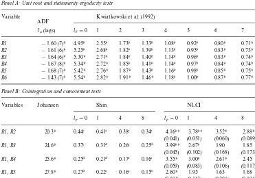
nonlinear error correction models (Granger and Swanson, 1996), threshold error correction models (Balke and Fomby, 1997), and the references contained therein. In this section, we do not estimate new varieties of nonlinear models, but rather, we illustrate the use of the nonlinear error-correction test discussed above. In order to do this, we examine data on the term structure of interest rates, which have been kindly provided to us by Heather Anderson. The data consist of monthly nominal yield to maturity "gures from the Fama Twelve Month Treasury Bill Term Structure File, for the period January 1970} Decem-ber 1988. Six variables, denoted R1}R6, are examined, and correspond to Treasury bills with one month to maturity, Treasury bills with two months to maturity, and so on, up to bills with 6 months to maturity. A detailed discussion of the data is given in Hall et al. (1992), as well as in Anderson (1997).
We consider three types of tests: (i) For the one-dimensional case, we con-struct both the ADF statistic for the null hypothesis of a unit root and the Kwiatkowski et al. (1992) test, described in Section 3, for the null of stationar-ity/ergodicity. (ii) For the two-dimensional case, we construct the Johansen
&trace'test statistic (1988, 1991) for the null of no cointegration, and the Shin (1994) test for the null of cointegration (comovement). For the latter cointegra-tion test, we compare the results using both the critical values in Shin (1994) and the critical values reported above. (iii) Also for the two-dimensional case, we perform the test for nonlinear cointegration described in Section 5.
Test results are reported in Table 6. Panel A contains ADF and Kwiatkowski et al. (1992) test results, where l
T denotes the number of lags used in the
computation of the estimated variance (see above). For the ADF test, q(k is reported, although test regressions without a constant were also run for all variables, and our"ndings did not di!er. Note that the outcomes of the ADF and the Kwiatkowski et al. (1992) tests agree. In particular, for all maturities, the unit root null hypothesis is not rejected (using the ADF test) while the null of stationarity ergodicity is consistently rejected (using the Kwiatkowski et al. (1992) test), regardless of the value ofl
T.
Panel B reports results based on cointegration and comovement tests. For the sake of brevity, only bivariate combinations which includeR1are reported on. Complete results are available from the authors. As mentioned above, the limiting distribution from Shin (1994) does not apply in the presence of neglected nonlinearity. Interestingly, even using the smaller critical values reported in Section 3 above, we fail to reject the null of stochastic comovement for 3 of 5 bivariate combinations, based on statistics constructed using l
T"4 and 8
(columns 5 and 6 of the table). Furthermore, for the other two bivariate combinations, use of the standard Shin (1994) critical values leads to a failure to reject at a 5% level (and in some cases a 1% level). These results agree with the theory posited by Hall et al. (1992) which suggests that any bivariate combination of our nominal interest rate series is cointegrated. Given these
Table 6
Empirical illustration: the term structure of interest rates!
Panel A: Unit root and stationarity ergodicity tests
Variable Kwiatkowski et al. (1992) ADF
q(k(lags) lT"0 1 2 3 4 5 6 7 8
R1 !1.60 (7)H 4.95H 2.55H 1.73H 1.33H 1.08H 0.92H 0.80H 0.71H 0.64H
R2 !1.61 (6)H 5.25H 2.68H 1.82H 1.39H 1.13H 0.95H 0.83H 0.73H 0.66H
R3 !1.64 (6)H 5.30H 2.71H 1.84H 1.40H 1.14H 0.96H 0.83H 0.74H 0.67H R4 !1.67 (8)H 5.34H 2.72H 1.85H 1.41H 1.14H 0.97H 0.84H 0.74H 0.67H
R5 !1.68 (7)H 5.42H 2.76H 1.87H 1.43H 1.16H 0.98H 0.85H 0.75H 0.68H R6 !1.43 (7)H 5.54H 2.82H 1.91H 1.46H 1.18H 1.00H 0.87H 0.77H 0.69H
Panel B: Cointegration and comovement tests
Variables Johansen Shin NLCI
l
T"0 1 4 8 lT"0 1 4 8
R1, R2 20.3H 0.44% 0.41% 0.38% 0.34% 4.16HH 3.78HH 3.52H 2.88H
(0.041) (0.051) (0.060) (0.089)
R1, R3 24.6H 0.37% 0.31$ 0.26% 0.25$ 3.99HH 2.67H 1.90 1.85
(0.045) (0.102) (0.168) (0.173)
R1, R4 25.6H 0.25$ 0.21$ 0.17# 0.16# 3.55H 3.00H 2.61H 2.45
(0.059) (0.083) (0.106) (0.117)
R1, R5 27.8H 0.27$ 0.22# 0.16# 0.15" 2.60H 1.95 1.63 1.68
(0.106) (0.162) (0.201) (0.194)
R1, R6 26.1H 0.40% 0.30$ 0.20# 0.18# 2.50 1.85 1.52 1.62
(0.113) (0.173) (0.217) (0.203)
!The data are monthly Treasury-Bill nominal yield to maturity"gures for the period 1970 : 1}1988 : 12.R1is the series for bills with one month to maturity,R2is the series for bills with two months to maturity, and so on up untilR6which is the series for bills with 6 months to maturity. Panel A contains augmented Dickey}Fuller (ADF) and Kwiatkowski et al. (1992) test statistics (as discussed above). For the ADF tests, the&lag augmentations'used is in brackets, chosen based on an examination of residual autocorrelations. All starred entires in Panel A correspond to evidence of a unit root (nonstationary-ergodicity) at the 5% level using critical values from Kwiatkowski et al. (1992) or MacKinnon (1991). In Panel B, the second column contains the Johansen (1988,1991) trace test statistics, where the associated vector autoregressions are estimated with a constant in the cointegrating relation, a linear determinstic trend in the data (results were the same without the deterministic trend), and 6 lags of each variable (similar results were found for the 12 lag case). Starred entries indicate rejection of the null hypothesis of no cointegration (in favor of cointegrating space rank of unity) using the 5% level critical value. The last 8 columns of Panel B contain Shin (1994) cointegration (comovement) and nonlinear error correction test statistics. For each of these two statistics, values are tabulated forl
T"0, 1, 4, 8.
"For the Shin-type tests superscrips&b'and&c'denote failure to reject the null hypothesis of cointegration (comovement) using the 5% and 1% (respectively) critical values in Section 3 of the paper.
#is the same as footnote&b'above.
$is the same as footnotes&b'and&c', but use the critical values of Shin (1994). For the nonlinear cointegration test (last 4 columns), values of the statistics, (mTq)2, which is used in the modi"ed Bonferroni bound of Hochberg (1988) de"ned as a"min
j/1,2,m(m!j#1)P(j), whereP(j)is thep-value of the test statistic, is reported. Here the values used forqareq"M2.0,
5.0, 8.0, 10.0N, so thatm"4. Modi"ed Bonferroni bounds are given in brackets below statistic values. Rejection of the null of linear cointegration in favor of the alternative of nonlinear cointegration at a 5% and 10% size are denoted by supersciptsH andHH, respectively.
error correction. The appropriate test statistics are reported in the last 4 col-umns of the table, with modi"ed Bonferroni bounds given in brackets below statistic values (see footnote to Table 6). Entries superscripted H(HH) denote rejection of the null hypothesis of linear cointegration (comovement) in favor of nonlinear cointegration at a 5% (10%) level. Thus, for the pair of series consisting of (R1, R2), some evidence of nonlinear cointegration is found, regard-less of the value ofl
T. Weaker evidence (i.e. rejections forsomeoflT) of nonlinear
cointegration is also found for (R1, R3), (R1, R4) and (R1, R5). Based on a com-parison of linear and nonlinear 1-step ahead forecast errors, Anderson (1997)
"nds evidence of nonlinear error correction among the variables considered here, consistent with our"ndings.
7. Conclusions
In this paper we introduce a class of nonlinear Markov processes character-ized by the sum of a linear component plus a bounded nonlinear component. In the one-dimensional case, the ergodicity of the process is equivalent to the absence of a unitary or explosive root, and in the multidimensional case the existence oflinear stochastic comovementis equivalent to the existence of coin-tegration.
We show that the statistic proposed by Kwiatkowski et al. (1992) has a well-de"ned limiting distribution under the null of general stationary-ergodic nonlin-ear processes, and has power not only against the alternative of integratedness, but also against the alternative of a more general nonlinear nonergodic process. We also show that the cointegration test statistic proposed by Shin (1994) is consistent, in our context, although the critical values of the test are quite di!erent from those tabulated by Shin (1994) for the linear case. Finally, we propose a consistent test for the null hypothesis of linear cointegration against the alternative of nonlinear cointegration (NLCI). In a series of Monte Carlo experiments, we"nd that the NLCI test has good"nite sample size and power. Further, in an illustration of the NLCI test in which we examine the term structure of interest rate, we"nd some evidence that bivariate models of interest rates of di!erent maturities may be nonlinearly cointegrated.
Acknowledgements
paper. We also owe special thanks to Herman Bierens for very useful sugges-tions, and to Heather Anderson for providing us with the data used in the illustration of our nonlinearity test. Swanson thanks the National Science Foundation and the Research and Graduate Studies O$ce at Pennsylvania State University for"nancial assistance. White's participation was supported by NSF grant SBR 9511253.
Appendix A
Proof of Proposition 2.1. Note"rst that
X
t"AXt~1#(g0(h10@Xt~12,hj0@Xt~1)!g0(0))#(et#g0(0)) "H(X
t~1)#(et#g0(0)).
Assume that the associated deterministic system, sayx
t, is given byxt"H(xt~1).
The proposition follows from Theroem 4.3 of Tong (1990), once we have shown that his assumptions B1}B3 are satis"ed. First, note that A1}A3 imply B2}B3. It remains to show that B1 is satis"ed. As lim
,x,?=(g0(x)!g0(0))/ExE"0 from
Theorem 1.3.5(a) in Kocic and Ladas (1993), it follows thatHis asymptotically stable at large, so that B1 is satis"ed. h
Proof of Proposition 2.3. (i) Let X
t"+tj/0At~jej#+tj/1At~jg0(h10@Xj~1,2, hj@0X
j~1)"XI t#g80,t. As XI t is a linear component, from Johansen (1988) and
from the Granger representation theorem (Engle and Granger, 1987), it follows that the Wold representation forXI tis*XI t"C(¸)e
t. Using the Beveridge and
Nelson (1981) decomposition it follows thatXI t"C(1)+tj/0e
j#CH(¸)et, where CH(¸)"+=
j/0(+=i/j`1Ci)¸j. Note also thatg80,T~1)Op(¹), as it is the sum of ¹bounded components. Now,XI
T/¹1@2NB1, whereB1is ap-dimensional mean
zero normal with covariance matrix equal to C(1)RC(1)@, and so is a non-degenerate random variable. Ifg80,T/¹1@2PRorg80,T/¹1@2P0, thenX
TPR
at rate¹1@2(ifXI Tis the component of higher order of probability) or at a rate faster than¹1@2(if the nonlinear component is of higher order than the linear component). Finally, consider the case in whichg80,T/¹1@2NG, whereGis either a nondegenerate or a degenerate random variable. As B
1 is a continuously
distributed nondegenerate random variable, P(u:B
1(u)"!G(u))"0. The
result follows directly.
(ii) The result follows from the fact that h@0X
t satis"es the assumptions of
Proposition 2.1. h
Proof of Proposition 2.4. Using the arguments from the proof of Proposition 2.3, and by setting A"I, it follows that EX
Furthermore,h@0X
t"h@0+tj/1ej#h@0+tj/1g0(h10@,2,hj@0Xj~1). Thus, noting that ¹~1@2(h@0+Tj/1e
j)Nh@0B2, whereB2is ap-dimensional mean zero normal with
covariance matrix equal toR, the result follows by the same argument used in the Proof of Proposition 2.3(i). h
Proof of Theorem 3.1. (i) First, note that
1
stationary mixing process, with mixing coe$cients decaying at a geometric rate. Furthermore, given A2, X
t is fourth-order stationary. Thus, by Lemma 1 in
Andrews (1991),X
t!E(Xt) satis"es his Assumption A. Given thatXM is¹1@2
-consistent for the true"rst moment, from Theorem 1(a) in Andrews (1991), it follows thats(2lTPp2
Xin Prob.The result then follows by the continuous mapping
theorem.
(ii) We need to show that the numerator ofS
T, say¹~2+Tt/1(+tj/1(Xj!XM ))2
explodes at a faster rate than doess(2
lT. First, consider the numerator. Under the
alternative,X
where =k
s"=s!:10=qdq, and = is a standard Brownian motion. Now, as
g
0is bounded, it follows that (1/¹4)+Tt/1(+tj/1+ji/1(g0(Xi~1)!g60))2"Op(¹).
Turning now to the denominator, note "rst from Kwiatkowski et al. (1992, p. 168), that it follows that
1
By comparing M and Qterm by term, observe that M&¹2Q. By the same
Thus, if the denominator explodes at rate ¹1`gl
T, g3[0, 1], the numerator
will explode at rate ¹2`g, and the ratio of the two will then explode at rate¹l~1
T . Note thatg"0 is the case in which either the linear component is
dominant or the two components, linear and nonlinear, are of the same order of probability. We have g'0 in the case in which the nonlinear component is dominant. h
Proof of Theorem 3.2. First, note that
Thus,
Proof of Theorem 3.3 (i) Let
mKt"(X Given Theorem 3.3(i), it follows that
1
0)"Op(1), and using the same argument used in the proof of
Theorem 3.1(i), it follows thats2
lTPp2l2inProb. The result follows.
1,t and X2,t are of the same order of probability (note that the
nonlinear components, g
0,1, g0,2, depend on the same argument, h@0Xt), bKT"O
p(1). Thus,s~2lT (1/¹2)+Tt/1(+tj/1mKj)2will explode at rate¹l~1T , by the same
regres-!(tK
We want to show that 1
(A.3) implies (4.6) in the text. Recall that underH
0, J¹(tKT!t0)"Op(1) and ¹(bKT!b
0)"Op(1). As the ninth term on the RHS of (A.2) converges to zero
faster than the"fth term, and the tenth term vanishes faster than the sixth, we can neglect them. Also, under H
0,X1,t"+tj/1l1,j, where E(l1,j)"0 for all j.
Note that when g
0 is a constant, then ¹1@2(tKT!t0)"Op(1) and ¹3@2(bK
T!b0"Op(1) and E(l1,j)O0 for allj. By twice applying the mean value
theorem, it turns out that
where Dkg denotes thekth derivative ofg with respect to its argument, and
cH"(!bH, 1)@, withbH3(b0,bKT),cHH"(!bHH, 1), andbHH3(bH,b0). Thus, the second term on the RHS of (A.2) can be written as
¹(bKT!b 0)
1
¹3@2 T + t/2
(X
1,t~1!XM1)qgt(Dg(c@0Xt~1q)!Dgc0) !¹(bKT!b
0)¹(bH!b0)
1
¹5@2 T + t/2
gt((X
1,t~1!XM1)2
]q2(D2g(cHHX
t~1q)!Dg2cHH), (A.4)
where Dgk
c0"(1/¹)+Dkg(c@0Xt~1q) and DgkcHH"(1/¹)+Dkg(c@HHXt~1q). Note
that Dg(c@0X
t~1q)!Dgc0is a zero mean strong mixing process, and that (from
Fact 2.5) the usual size conditions required by the invariance principle hold. Also, by a similar argument as that used in Hansen (1992b, Proof of Theorem 4.1),
1
¹ T + t/2
(X
1,t~1!XM1)qgt(Dg(c@0Xt~1!Dgc0"Op(1),
so that the"rst term in (A.4) isO
p(¹~1@2). Also, note that the absolute value of
the second term in (A.4) is majorized by
¹DbK
T!b0D¹DbH!b0DsuptDD2g(c@HHXt~1q) !Dg2cHHDq2 1
J¹suptDgtD
1
¹2 T + t/2
(X
1,t~1!XM1)2. (A.5)
Now, ¹DbH!b
0D)¹DbKT!b0D"Op(1) and (1/J¹) suptDgtD"op(1). It follows
that the expression in (A.5) iso
p(1), and thus the expression in (A.4) is alsoop(1).
Now, consider the eighth term on the RHS of (A.2), which can be written as (tKT!t
0)(bKT!b0)
1
J¹ T + t/2
qX1,t~1(c@0X
t~1!c@0XM )(Dg(c@0Xt~1q)!Dgc0)
!(tKT!t
0)(bKT!b0)(bH!b0)
1
J¹+(X1,t~1
!XM1)2q2
](c@0X
t~1!c@0XM )(D2g(c@HHX1,t~1q)!Dg2cHH)"o p(1),
using the same majorization argument which is used above. By an analogous argument, the fourth, "fth and sixth terms are o
p(1). Given that ¹(bKT!b
we have that s2
lTPp20 in Prob. The result follows. Note also that when g0
is a nonzero constant, ¹1@2(tK!t
0)"Op(1), ¹3@2(bKT!b0)"Op(1), and
E(l1,j)O0 for all j. Thus, the same arguments used above apply when g 0 is
a nonzero constant.
(ii) Under the alternative,X
1,t"nt#+tj/1(l1,t!n)"nt#+tj/1uj. AsX1,tis
dominated by the deterministic component, ¹3@2(bKT!b
0)"Op(1). Further,
J¹(tKT!tH)"O
p(1), where tHOt0. Now all of the terms on the RHS of
(A.2), except for the"rst and the seventh areo
p(1), by an argument analogous to
that used in part (i), and by the law of large numbers for strong mixing processes, (1/¹)+Tt/2(g(c@0X
t~1q)!g6)!M~1c@0Xc0@XMc@0gXt~1)gtPMO0. The result then
fol-lows. h
References
Altissimo, F., Violante, G.L., 1995. Persistence and Nonlinearity in GNP and Unemployment: an Endogeneous Delay Threshold VAR, Mimeo, University of Pennsylvania.
Anderson, H.M., 1997. Transaction costs and nonlinear adjustment towards equilibrium in the US treasury bill market. Oxford Bulletin of Economics and Statistics 59, 465}480.
Anderson, H.M., Vahid, F., 1988. Testing multiple equation systems for common nonlinear compo-nents. Journal of Econometrics 84, 1}36.
Andrews, D., 1991. Heteroskedasticity and autocorrelation consistent covariance matrix estimation. Econometrica 59, 817}858.
Athreya, K.B., Pantula, S.G., 1986. Mixing properties of Harris chains and autoregressive processes. Journal of Applied Probability 23, 880}892.
Balke, N.S., Fomby, T.B., 1997. Threshold cointegration. International Economic Review 38, 627}645.
Beveridge, S., Nelson, C., 1981. A new approach to decomposition of economic time series into permanent and transitory components with particular attention to measurement of the business cycle. Journal of Monetary Economics 7, 151}174.
Bierens, H.J., 1990. A consistent conditional moment test of functional form. Econometrica 58, 1443}1458.
Corradi, V., 1995. Nonlinear transformations of integrated time series: a reconsideration. Journal of Times Series Analysis 16, 539}549.
Domowitz, I., El-Gamal, M.A., 1993. A consistent test for stationary-ergodicity. Econometric Theory 9, 589}601.
Domowitz, I., El-Gamal, M.A., 1997. A consistent nonparametric test of ergodicity for time series with applications. Mimeo, Northwestern University.
Engle, R.F., Granger, C.W.J., 1987. Co-integration and error correction: representation, estimation and testing. Econometrica 55, 547}557.
Ermini, L., Granger, C.W.J., 1993. Some generalization of the algebra ofI(1) processes. Journal of Econometrics 58, 369}384.
Granger, C.W.J., 1995. Modelling nonlinear relationships between extended-memory variables. Econometrica 63, 265}279.
Granger, C.W.J., Hallman, J., 1991. Long memory series with attractors. Oxford Bulletin of Economics and Statistics 53, 11}26.


![Table 5Nonlinearity test performance:� g�(x)"sin(x) if �x�)�/2, otherwise g�(x)"[2/(1#e��)]!1e�f�f�T"100T"250T"500l�"l�1l�"l�2l�"l�3l�"l�1l�"l�2l�"l�3l�"l�1l�"l�2l�"l�30.2!2.00.00.1460.1210.0800.5210.4930.4420.9230.9190.9030.4!2.00.00.1370.1160.0760.5510.5](https://thumb-ap.123doks.com/thumbv2/123dok/3106732.1376868/22.468.56.585.109.281/table-nonlinearity-test-performance-sin-t-t-t.webp)