MULTI-SOURCE MULTI-SCALE HIERARCHICAL CONDITIONAL RANDOM FIELD
MODEL FOR REMOTE SENSING IMAGE CLASSIFICATION
Z. Zhanga, M.Y. Yangb, M. Zhoua a
Academy of OptoElectronics, Chinese Academy of Sciences, Beijing, China bInstitute for Information Processing (TNT), Leibniz University Hannover, Germany
WG III/3
KEY WORDS:Classification, Fusion, Multisensor, LIDAR, Hierarchical, Vision, Performance
ABSTRACT:
Fusion of remote sensing images and LiDAR data provides complimentary information for the remote sensing applications, such as object classification and recognition. In this paper, we propose a novel multi-source multi-scale hierarchical conditional random field (MSMSH-CRF) model to integrate features extracted from remote sensing images and LiDAR point cloud data for image classifica-tion. MSMSH-CRF model is then constructed to exploit the features, category compatibility of multi-scale images and the category consistency of multi-source data based on the regions. The output of the model represents the optimal results of the image classifica-tion. We have evaluated the precision and robustness of the proposed method on airborne data, which shows that the proposed method outperforms standard CRF method.
1. INTRODUCTION
In the fields of photogrammetry and remote sensing, there exist many sources of earth observation data with the different charac-teristics of targets on the ground. For a long period, integration of the multi-source data reasonably and effectively has been an active topic. Fusion of remote sensing images and LiDAR data provides complimentary information for the remote sensing ap-plications, such as object classification and recognition.
Many methods have been developed for the fusion of remote sensing images and LiDAR data. In general those methods are classified into three categories, namely image fusion (Parmehr et al., 2012), feature fusion (Dalponte et al., 2012, Deng and Su, 2012), and decision fusion (Huang et al., 2011, Shimoni et al., 2011). The methods for image fusion include different resolu-tion data sampling and registraresolu-tion, so the processing is time-consuming, and the accuracy is affected by the accuracy of reg-istration, which reduces the performance of the subsequent im-age classification. In the feature fusion methods, the features are usually extracted independently from different data source, and the fusion lacks consideration of correspondence of location and contextual information, by which the classification could be im-proved.
In order to overcome the limitations of the aforementioned meth-ods, we present a novel multi-source multi-scale hierarchical con-ditional random field (MSMSH-CRF) model to fuse features ex-tracted from remote sensing images and LiDAR point cloud data for image classification. In this paper, the majorcontribution is that both the category compatibility of the multi-scale image in a hierarchical structure and the category consistency of multi-source data are considered in the MSMSH-CRF model. The fol-lowing sections are organized as follows. The related work is discussed in Section 2.. In Section 3., the MSMSH-CRF model is presented in detail. In Section 4., experimental results are pre-sented. Finally, this contribution of this paper is concluded and the future work is discussed in Section 5..
2. RELATED WORK
In order to make full use of multi-source data for image classifica-tion and object recogniclassifica-tion, many feature-based fusion methods have been proposed. One of the classic tools are graphical mod-els (Bishop, 2006), i.e. probabilistic modmod-els defined on a graph describing the conditional dependence structure between random variables. As the one branch of the graphical model, Markov Random Fields (MRFs) have been used for image interpretation since 1986 (Besag, 1986), and their limiting factor only allow-ing for local image features has been overcome by Conditional Random Fields (CRFs) (Lafferty et al., 2001), where arbitrary features can be used for classification. CRFs have the ability to discriminatively model contextual dependencies, conditioned on observations, for capturing global as well as local image con-text, which makes them suitable for accurate labeling (Perez et al., 2012). Therefore, they have been receiving more and more attention in recent years (Yang and F¨orstner, 2011b, Zhang et al., 2012, Niemeyer et al., 2014).
which is a flexible method for obtaining a reliable 3D classifica-tion in complex urban scenes. These methods exploit both spa-tial and hierarchical structures of objects in images. Considering the limitation of visual feature information from the images, the classification results could be potentially improved by incorporat-ing information from different source data, such as the elevation information in LiDAR data and the spectral information in the hyperspectral images.
3. MSMSH-CRF MODEL FOR AUTOMATIC CLASSIFICATION
In this section, we start by presenting the graphical model to inte-grate an image and LiDAR data, so-called MSMSH-CRF model, with corresponding energy function. Then, we describe the model construction process. Afterward, we will derive the features from each region obtained from the unsupervised segmentation algo-rithm. Then, we will give particular formulations for each of the unary, pairwise, hierarchical potentials respectively. Finally, we will discuss the learning and inference of this graphical model.
3.1 MSMSH-CRF model
In the field of image analysis, the regions of interest are usually detected independently, but considering the relative position tween regions in single source data and the correspondence be-tween regions from multi-source data, the labeling of every re-gion should not be independent. The CRF model is an effective way to solve the problem of prediction of the non-independent labeling for multiple outputs, and in this model, all the features can be normalized globally to obtain the global optimal solution.
Based on the standard CRF model, we propose the MSMSH-CRF model to learn the conditional distributions over the class labeling given an image and corresponding LiDAR data, and the model al-lows us to incorporate different features and correspondence in-formation in a single unified model, as illustrated in Figure 3. The conditional probability of the class labels c given an image X and LiDAR data L, which has a distribution of the Gibbs form, is defined as follows
P(c|X,L, θ) = 1
Z(θ, X, L)exp(−E(c|X, L, θ)) (1)
And the energy function
E(c|X,L, θ) =X
i∈S
E1(ci, xi, θ1)
+ X
(i,j)∈N
E2(ci, cj, xi, xj, θ2)
+ X
(i,k)∈M
E3(ci, ck, xi, xk, θ3)
+ X
(i,t)∈H
E4(ci, ct, xi, lt, θ4)
(2)
whereθ = {θ1, θ2, θ3, θ4}is the vector of model parameters,
Z(θ,X,L)is the partition function,i, jandkrespectively index regionsxi, xjandxkin the image, which correspond to nodes in
the graph, andtindex regionsltin the LiDAR data, which also
correspond to nodes in the graph. S is the set of all the nodes in image level of the graph,N is the set of corresponding pairs collecting neighborhood in both images and LiDAR data,M is the set of pairs collecting parent-child relations between regions with neighboring scales, andHis the set of corresponding pairs collecting neighborhood in both images and LiDAR data. E1is the unary potentials, which represent relationships between class
labels and the observed data,E2is the pairwise potentials, repre-senting relationships between class labels of neighboring regions within each scale.E3is the multi-scale hierarchical pairwise po-tential, which represents corresponding relationships between re-gions in neighboring scales of images. E4 is the multi-source hierarchical pairwise potential, representing corresponding rela-tionships between images and LiDAR data.
3.2 Model construction
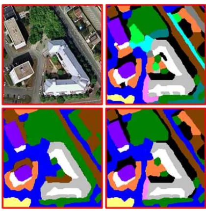
In order to integrate features extracted from multi-source data for image classification, the MSMSH-CRF graphical model is con-sist of two levels: Image level and LiDAR level. In Image level, Texton is utilized to distinguish between different regions effec-tively and obtain the different segmented regions, which form all the nodes in image level of the graph. Meanwhile, we can change the amount of channels of the Texton filter (Shotton et al., 2009) to get different results which are similar to the multi-scale seg-mentation, and Figure 1 shows the example results of our algo-rithm. The neighborhood in Image level is defined as the rela-tionship of two regions which have the common edge. In LiDAR level, the mean shift algorithm is used to get the flat regions corre-sponding to continuous planes of different targets in LiDAR data, which form all the nodes in LiDAR level of the graph.
Figure 1: The example region images of Texton segmentation results at scale 1, 2, 3 respectively. The color of each region is assigned randomly that neighboring regions are likely to have different colors. Top row left: Original image,Top row right: segmentation result at scale 3. Bottom row left: segmentation result at scale 1,Bottom row right: segmentation result at scale 2.
For describing the consistency of multi-source data, we firstly choose the optimal scale of images to match with the LiDAR data. Assuming that there is a registration of multi-source data acquired on the same airborne platform, such as the algorithm introduced in literature (Mastin et al., 2009), and we calculate the center of each region (or line)RLiin the depth image converted from
LiDAR data, and the center should be inside the region (or line) and at the symmetric axis. Then based on the relative position of the centers, the corresponding regions (or lines)RLiain
by
a∗= arg min
a
X
s∈{RIi∪RIia}
|RIi(s)−RIia(s)| (3)
and
RLi(s) ={
1, s∈RLi,
0, s /∈RLi , RLia(S) ={
1, s∈RLia,
0, s /∈RLia
(4)
whereiindex the sequence number of all regions (or lines) in the depth image converted from the Mean Shift Feature (MSF) or Alpha Shape Feature (ASF) of LiDAR data.
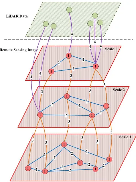
Therefore, the MSMSH-CRF graphical model is constructed as follows, illustrated in Figure 3. Firstly, typical features are de-rived from the interest regions in multi-source data, where the re-gions are generated by an unsupervised segmentation algorithm. In the graphical model, the nodes correspond to regions. The blue edges represent the dependencies between neighboring re-gions, and the orange edges indicate the hierarchical relations be-tween regions at different scales in a multi-scale segmentation. Purple edges indicate the hierarchical relations between regions from multi-source data, where the optimal scale of images is se-lected to match the LiDAR data. The MSMSH-CRF model is constructed to exploit the features and category compatibility of scale images as well as the category consistency of multi-source data based on regions. The output of the model represents the optimal results of the image classification.
Figure 2: The example image of illustrating the procedure of choosing the optimal scale image to match the LiDAR data.
3.3 Features
Four types of features are extracted, namely the line features (LF), the texture features (TF), the mean shift features (MSF), and alpha shape features (ASF). The line features (LF) and the texture features (TF) are extracted from remote sensing images, whereas the mean shift features (MSF) and alpha shape features (ASF) are from LiDAR data.
Line Features (LF) Shape features, in particular line features, not only describe the structures of targets directly, but also are sta-ble to light change, color change, etc. As a new and effective one of line features, the LSD (Line Segment Detector) (Grompone and Randall, 2010) can be used to give accurate results extracted, a controlled number of false detections, and requires no param-eter tuning. In the method, the level-line orientation is defined and calculated by gradient magnitude, and then the pixels with the same level-line orientation are merged to cover the so-called line support regions, in which all the pixels are regarded as a long
Figure 3: Illustration of the MSMSH-CRF model architecture. In Image level, red nodes (# 1) correspond to image regions, blue edges (# 2) linking red nodes represent the dependency between neighboring regions, and orange edges (# 3) linking red nodes in multi-scale indicate the hierarchical relation between regions at different scales corresponding to the multi-scale segmentation. In LiDAR level, green nodes represent the extracted regions. Purple edges (# 4) linking red and green nodes indicate the hierarchi-cal relation between regions from multi-source data, where the optimal scale of images is selected to match the LiDAR data.
continuous segment. In accordance with the method introduced in (Grompone and Randall, 2010), we can calculate the response value of LSD at each pixel, denoted byLF(s).
the MSF is introduced in (Georgescu et al., 2003), all the LiDAR points are clustered in different regions, and the elevation of all points in one region are assigned as the same value which is the mean of all the ones.
Alpha Shape Features (ASF) There are many methods for ex-tracting the boundary of LiDAR data. Compared with other algo-rithms (Berger, 2012, Kong et al., 2012), Alpha Shapes algorithm works effectively in inner and outer boundaries extraction from LiDAR data with convex and concave polygon shape. Moreover, it can keep fine features of buildings adaptively and filter the foot-prints of non-building. Based on the MSF regions obtained, the alpha shape algorithm is used to extract the boundary contour of each region, and then the Delaunay triangulation is used to get the line feature. The extraction of the ASF refers to (Shen et al., 2011), similar to the MSF, all the points in one lines have the same elevation which is the mean of all the ones.
3.4 Unary potentials
The unary potentials consist of two element: LF and TF poten-tials, predict the labelciof the regionxibased on the imageX
E1(ci, xi, θ1) =LF(ci, xi, θLF) +T F(ci, xi, θT F) (5)
whereLF(ci, xi, θLF)is the LF potential andT F(ci, xi, θT F)
is the TF potential, andθ1={θLF, θT F}is the vector of model
parameters.
LF Potentials The LF potentials capture the (relatively weak) dependence of the class label and the boundaries of targets on the response value of LSD and absolute location of the pixel in the image. We can get the line segment imageLF I(s)by calculating the response value of LSDLFsof each pixelsin the regionxi.
The LF potentials take the form of a look-up table with an entry for each class ci and value of LSDLFsand pixel locations
LF(ci, xi;θLF) =−log X
s∈xi
θLF(ci, LFs, s) (6)
where the parameterθLF represents the relationship among the
value of each pixelLFs, namelyLF I(s), the pixel locations
and the labelci.
TF Potentials Based on the Joint Boost algorithm, an adapted version of boosting learning algorithm, we can obtain the clas-sifier of Texton, to which the responses are used directly as a potential in the MSMSH-CRF model, so that
T F(ci, xi;θT F) =−log X
s∈xi
P(ci|T Fs) (7)
whereT Fscorresponds to the response of classifier at each pixel
s, andP(ci|T Fs)is the normalized distribution given by the
clas-sifier using the learned parametersθT F.
3.5 Pairwise potentials
The pairwise potentials describe category compatibility between neighboring regionsxiandxjobtained from the line segment
im-ageLF I(s), and the responses of Texton classifier on the image X.
Pairwise Potentials of LF Based on the line segment image LF I(s), we can calculate the pairwise potentials of LF as the form of the contrast-sensitive Potts model (Boykov and Jolly, 2001)
of the pixel value between regionsxiandxjin the LF images,
Ni is the number of regions neighbored to regioni, Njis the
number of regions neighbored toj, andσ(·)is a 0-1 indicator function, and the number 6 in Eq. (9) is set empirically. The pairwise potentialsP LF(ci, cj, xi, xj, θP LF)are scaled byNi
andNjto compensate for the irregularity of the graph.
Pairwise Potentials of TF Similar to the pairwise potentials of LF, the pairwise potentials of TF take the form of the contrast-sensitive Potts model:
of the value of Texton classifier at each pixel between regions xi and xj in the results of marked images, and the number 4
in Eq. (10) is set empirically. The pairwise potentialsP T Fare scaled byNi and Nj to compensate for the irregularity of the
graph.
3.6 Multi-scale hierarchical pairwise potentials
From the pairwise potentials in Section 3.5, there is a lack of longer range contextual relationship in the graphical modeling. To overcome those local restrictions, we analyze the image at multiple scales to enhance the model by evidence aggregation on a local to global level. Furthermore, we integrate multi-scale pair-wise potentials to regard the hierarchical structure of the regions.
Based on results of multi-scale segmentation, the multi-scale hi-erarchical pairwise potentials describe category compatibility be-tween hierarchically neighboring labelsciandckgiven the image
X, which take the form of the contrast-sensitive Potts model:
E3(ci, ck, xi, xk, θ3) =
θ3·[1 + 4 exp(−2m(xi, xj))]σ(ci6=ck)
(11)
whereθ3is the weight factor,m(xi, xj)is the Euclidean metric
of the value of Texton classifier between regionsxi and xj in
the results of marked images, and the number 4 in Eq. (11) is set empirically. Multi-scale hierarchical pairwise potentials act as a link across scale, facilitating propagation of information in the model.
3.7 Multi-source hierarchical pairwise potentials
denoted asHP P(ci, ct, xi, lt, θp)andHP L(ci, ct, xi, lt, θl)
re-Hierarchical pairwise potentials of planar features Based on the TF results of the optimal scale image, we firstly normalize the valueT Fs(xi)of Texton classifier of each pixelsin the region
xito getN T Fs(xi):
N T Fs(xi) =T Fs(xi)/T Fmax (13)
whereT Fmaxis the maximum value of Texton classifier of each
pixel in the image.
In the MSF results of LiDAR data, elevations of different re-gions are obtained, and the normalized elevationN M SF(lt)of
all points in the regionsltextracted is calculated:
N M SF(lt) =M SF(lt)/M SFmax (14)
whereM SF(lt) is the elevation of all points in the regionlt,
andM SFmaxis the maximum elevation of all flat regions in the
LiDAR data.
So based on the normalized valueN T Fs(xi)andN M SF(lt),
the hierarchical pairwise potentials of planar features is defined by
comparative item,<·>is the averaging operator, andθpis the
weight.
Hierarchical pairwise potentials of linear features The hier-archical pairwise potentials of linear features take the form as
HP L(ci, ct, xi, lt, θt) =
ized value from the LF results of the optimal scale image, and N ASF(lt)is the normalized value from the ASF of LiDAR data.
3.8 Parameter Learning
In this paper, piecewise training method (Sutton and McCallum, 2005) is adopted for the learning of the parameters of MSMSH-CRF model. This method divides the MSMSH-MSMSH-CRF model into pieces corresponding to the different terms in Eq. (2). Each of these pieces is then trained independently, as if it were the only term in the model.
Parameters of LF Potentials The formula for calculating the parameters of LF Potentials respectively for each image is defined as where the small positive integerwLF is set to 0.1 in practice.
Parameters of TF Potentials The learning of parameters of TF Potentials is based on Joint Boost algorithm, and an excel-lent detailed treatment of the learning process is given in liter-ature (Shotton et al., 2009), but we briefly describe it here for completeness. Each training examples(a pixel in a training im-age) is paired with a target valueZc
s ∈ {−1,+1}(+1if the
exampleshas ground truth classc,−1otherwise) and assigned a weightωc
sspecifying its classification accuracy for classc
af-ter iaf-teration of boosting. Each round of iaf-teration chooses a new weak learner by minimizing an error function incorporating the weights. The training examples are then re-weightedωc
s to
re-flect the new classification accuracy. This procedure emphasizes poorly classified examples in subsequent rounds of iteration, and ensures that over many rounds, the classification for each train-ing example approaches the target value and the parameters are optimal.
Parameters of other potentials The parameters of other po-tentials of MSMSH-CRF model,θP LF, θP T F, θ3, θpandθl, are
selected manually such that the classification error is minimized on the training set.
3.9 Model Inference
Given a set of parameters learned for the MSMSH-CRF model, the optimal labelingc∗, which minimizes the energy function in Eq. (2), is found by applying the alpha-expansion graph-cut algo-rithm (Boykov et al., 2001, Boykov and Jolly, 2001).
4. EXPERIMENTS
In this section, experiments are performed on the Beijing Air-borne Data (Zhang et al., 2013), to evaluate the performance of the proposed method.
4.1 Dataset
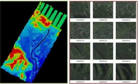
We conduct experiments to evaluate the performance of the MSMSH-CRF model on the Beijing Airborne Data (Zhang et al., 2013), which include remote sensing images with a resolution of 0.12m and LiDAR data with a point density of 4 points/m2, as illustrated in Figure 4. The objects in all images correspond to one of three classes: Building, Road and Vegetation. These classes are typical objects appearing in airborne images. In the experiments, we take the ground-truth label of a region to be the majority vote of the ground-truth pixel labels, and randomly divide the images into a training set with 50 images and a testing set with 50 images.
Figure 5: The classification result from the MSMSH-CRF model on the Beijing Airborne Data.Left: remote sensing image,Middle: LiDAR point cloud,Right: classification result (red - building, blue - road, green - vegetation).
Method Accuracy (%)
(Shotton et al., 2009) 64.2 (Zhang et al., 2013) 73.6
Ours 83.7
Table 1: Average pixelwise accuracy of three methods on the Bei-jing Airborne Data.
4.2 Results
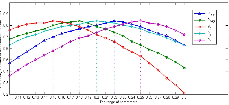
Figure 5 shows the example results of MSMSH-CRF classifica-tion method. The average pixelwise accuracy on the testing set is given in Table 1. The average classification accuracy of our method is 83.7%, which has 10.1% gain w.r.t. the accuracy of the MSHCRF model (Zhang et al., 2013) and 19.5% gain w.r.t. the accuracy of the standard CRF model (Shotton et al., 2009). The parameter, learned by cross validation on the training set, are θP LF = 0.22, θP T F = 0.18, θ3 = 0.15, θp = 0.2, and
θl = 0.25. For the fairness of comparison, both the training
set and the testing set are same for MSMSH-CRF, MSHCRF and standard CRF respectively. Figure 6 shows the classifica-tion accuracy with different parameters, with only one parameter is changing while the others are fixed.
Table 2 shows the confusion matrix obtained by applying stan-dard MSMSH-CRF model to the whole test dataset. Accuracy values in the table are computed as the percentage of image pix-els assigned to the correct class label, ignoring pixpix-els labeled as void in the ground truth. Compared to the confusion matrices of standard CRF model and MSHCRF model in Table 3 and Table 4 respectively, the MSMSH-CRF model yields significant improve-ment on all three classes for integrating multi-scale hierarchical information of the regions in the images. Table 5 shows the per-formance comparison when dropping one types of potentials in the MSMSH-CRF model.
5. CONCLUSIONS
In conclusion, this paper presents a novel source multi-scale hierarchical conditional random field model for automatic classification of remote sensing images. The main contributions of this work are summarized as follows: a novel CRF-based mod-eling scheme exploiting the complementarity of multi-source data
building road vegetation
building 78.3 11.9 9.8
road 9.5 85.9 4.6
vegetation 9.7 8.7 81.6
Table 2: Pixelwise accuracy of the MSMSH-CRF classification on the Beijing Airborne Data. The confusion matrix shows clas-sification accuracy for each class (rows) and is row-normalized to sum to 100%. Row labels indicate the true class, and column labels indicate the predicted class.
building road vegetation
building 63.7 19.2 17.1
road 22.4 67.0 10.6
vegetation 11.3 15.2 73.5
Table 3: The confusion matrix: pixelwise accuracy of the stan-dard CRF classification on the Beijing Airborne Data.
building road vegetation
building 70.1 15.8 14.1
road 14.4 77.3 8.3
vegetation 12.3 13.8 73.9
Table 4: The confusion matrix: pixelwise accuracy of the MSHCRF classification on the Beijing Airborne Data.
Potentials Accuracy (%)
With all potentials 83.7
Removing the pairwise potentials 63.9 Removing the multi-scale
hierarchical pairwise potentials 73.6 Removing the Multi-source
hierarchical pairwise potentials 70.1
Figure 6: The classification accuracy with different parameters, with only one parameter is changing while the others are fixed.
such as the texture in remote sensing images and the elevation in LiDAR data. To exploit different levels of contextual information in images, the multi-scale hierarchical potentials are proposed in our model, which is then enhanced by evidence aggregation from a local to global level. Considering the interrelation of the same objects in remote sensing images and LiDAR data, multi-source hierarchical potentials are proposed in our model to make full use of the category consistency of multi-source data. We have evalu-ated the precision and robustness of the proposed approach on air-borne data, which shows that the proposed method outperforms standard CRF method. However, feature extraction is crucial to the final classification accuracy. Feature selection is done in an ad-hoc fashion in the current stage. In our future work, we are in-terested in automatic feature selection that may further improve the classification performance.
ACKNOWLEDGEMENTS
The work is partially funded by National Natural Science Fund of China (Grant No. 40901177). The authors gratefully acknowl-edge these supports. The authors thank Dr. Franz Rottensteiner for his valuable assistance.
REFERENCES
Berger, C., 2012. Toward rich geometric map for slam: Online detection of planes in 2d lidar. In: Proceedings of the Inter-national Workshop on Perception for Mobile Robots Autonomy (PEMRA).
Besag, J., 1986. On the statistical analysis of dirty pictures. Jour-nal of the Royal Statistical Society. Series B (Methodological) pp. 259–302.
Bishop, C., 2006. Pattern recognition and machine learning. Springer.
Boykov, Y., Veksler, O. and Zabih, R., 2001. Fast approximate energy minimization via graph cuts. IEEE Transactions on Pat-tern Analysis and Machine Intelligence 23, pp. 1222–1239. Boykov, Y. Y. and Jolly, M.-P., 2001. Interactive graph cuts for optimal boundary & region segmentation of objects in nd images. In: IEEE International Conference on Computer Vision (ICCV), pp. 105–112.
Comaniciu, D. and Meer, P., 2002. Mean shift: A robust ap-proach toward feature space analysis. IEEE Transactions on Pat-tern Analysis and Machine Intelligence 24(5), pp. 603–619.
Dalponte, M., Bruzzone, L. and Gianelle, D., 2012. Tree species classification in the southern alps based on the fusion of very high geometrical resolution multispectral / hyperspectral images and lidar data. Remote Sensing of Environment 123, pp. 258–270.
Deng, F.and Li, S. and Su, G., 2012. Classification of re-mote sensing optical and lidar data using extended attribute pro-files. IEEE Journal of Selected Topics in Signal Processing 6(7), pp. 856–865.
Georgescu, B., Shimshoni, I. and Meer, P., 2003. Mean shift based clustering in high dimensions: A texture classification ex-ample. In: IEEE International Conference on Computer Vision (ICCV), pp. 456–463.
Grompone, R., J. J. M. J. and Randall, G., 2010. Lsd: A fast line segment detector with a false detection control. IEEE Transactions on Pattern Analysis and Machine Intelligence 32(4), pp. 722–732.
Huang, X., Zhang, L. and Gong, W., 2011. Information fusion of aerial images and lidar data in urban areas: vector-stacking, re-classification and post-processing approaches. International Journal of Remote Sensing 32(1), pp. 69–84.
Kong, D., Xu, L., Li, X. and Xing, W., 2012. Estimation of cluster centers on building roof from lidar footprints. In: IEEE International Conference on Imaging Systems and Techniques, pp. 254–258.
Lafferty, J., McCallum, A. and Pereira, F., 2001. Conditional random fields: Probabilistic models for segmenting and labeling sequence data. In: International Conference on Machine Learn-ing (ICML), pp. 282–289.
Mastin, A., Kepner, J. and Fisher, J., 2009. Automatic registration of lidar and optical images of urban scenes. In: IEEE Conference on Computer Vision and Pattern Recognition (CVPR), pp. 2639– 2646.
Parmehr, E. G., Zhang, C. and Fraser, C. S., 2012. Automatic registration of multi-source data using mutual information. In: ISPRS Annals of the Photogrammetry, Remote Sensing and Spa-tial Information Sciences, ISPRS Congress, pp. 301–308.
Perez, M., Chan, J. and Sahli, H., 2012. Multiscale conditional random fields for supervised region based labeling and classifi-cation. In: IEEE International Geoscience and Remote Sensing Symposium (IGARSS), pp. 1769–1772,.
Schindler, K., 2012. An overview and comparison of smooth labeling methods for land-cover classification. IEEE Transactions on Geoscience and Remote Sensing 50(11), pp. 4534–4545.
Shen, W., Zhang, J. and Yuan, F., 2011. A new algorithm of building boundary extraction based on lidar data. In: IEEE Inter-national Conference on Geoinformatics, pp. 1–4.
Shimoni, M., Tolt, G., Perneel, C. and Ahlberg, J., 2011. Detec-tion of vehicles in shadow areas using combined hyperspectral and lidar data. In: IEEE International Geoscience and Remote Sensing Symposium (IGARSS), pp. 4427–4430.
Shotton, J., Winn, J., Rother, C. and Criminisi, A., 2009. Tex-tonboost for image understanding: Multi-class object recognition and segmentation by jointly modeling texture, layout, and con-text. International Journal of Computer Vision 81(1), pp. 2–23.
Sutton, C. and McCallum, A., 2005. Piecewise training for undi-rected models. In: Uncertainty in Artificial Intelligence (UAI), pp. 568–575.
Yang, M. Y. and F¨orstner, W., 2011a. A hierarchical conditional random field model for labeling and classifying images of man-made scenes. In: IEEE International Conference on Computer Vision Workshops (ICCV Workshops), pp. 196–203.
Yang, M. Y. and F¨orstner, W., 2011b. Regionwise classification of building facade images. In: Photogrammetric Image Analysis, Springer, pp. 209–220.
Zhang, Z., Yang, M. Y. and Zhou, M., 2013. Multi-source hi-erarchical conditional random field model for feature fusion of remote sensing images and lidar data. In: International Archives of the Photogrammetry, Remote Sensing and Spatial Information Sciences; ISPRS Hannover Workshop, pp. 389–392.