A UNIFIED FRAMEWORK FOR DIMENSIONALITY REDUCTION AND
CLASSIFICATION OF HYPERSPECTRAL DATA
Pavan Kolluru a, Kamal Pandey b,*, Hitendra Padaliac
a Indian Institute of Remote Sensing, Indian Space Research Organization, Dehradun([email protected]) b Indian Institute of Remote Sensing, Indian Space Research Organization, Dehradun([email protected])
c Indian Institute of Remote Sensing, Indian Space Research Organization, Dehradun([email protected])
Commission VI, WG VI/4
KEY WORDS:
Unified Framework, SVMDRC, Dimensionality Reduction, Intrinsic Dimensionality
ABSTRACT:
The processing of hyperspectral remote sensing data, for information retrieval, is challenging due to its higher dimensionality. Machine learning based algorithms such as Support Vector Machine (SVM) is preferably applied to perform classification of high dimensionality data. A single-step unified framework is required which could decide the intrinsic dimensionality of data and achieve higher classification accuracy using SVM. This work present development of a SVM-based dimensionality reduction and classification (SVMDRC) framework for hyperspectral data. The proposed unified framework was tested at Los Tollos in Rodalquilar district of Spain, which have predominance of alunite, kaolinite, and illite minerals with sparse vegetation cover. Summer season image was utilized for implementing the proposed method. Modified broken stick rule (MBSR) was used to calculate the intrinsic dimensionality of HyMap data which automatically reduce the number of bands. Comparison of SVMDRC with SVM clearly suggests that SVM alone is inadequate in yielding better classification accuracies for minerals from hyperspectral data rather requires dimensionality reduction. Incorporation of modified broken stick method in SVMDRC framework positively influenced the feature separability and provided better classification accuracy. The mineral distribution map produced for the study area would be useful for refining the areas for mineral exploration.
* Corresponding author.
1. INTRODUCTION
In the recent decade, advances in hyperspectral technology have increased the perception and knowledge of the earth’s surface. The spectroscopy integrated into remote sensing systems has offered high spectral resolutions to capture subtle details of objects thereby providing better discrimination and identification of the targets.
Some of the most important factors that make the usage of hyperspectral data complex are data volume, atmospheric distortions and high dimensionality. With the advancement in computation processing speed, the large volume of data can be handled. Another issue with hyerperspectral data is atmospheric corrections which also can be performed accurately for airborne hyperspectral data. The higher dimensionality of data suffers information redundancy and noisy. The advantages of dimensionality deduction is that it reduces the number of dimensions because a small portion of data can explain most of the variance of the image, while the original features of the data are preserved (Burgers et al,2009).
After dimensionality reduction, the optimum number of bands are to be selected which have the total data content of the original image. This is done by considering the virtual dimensionality of the reduced image. Intrinsic dimensionality, because of some undesirable properties, produces unreasonable results in case of hyperspectral images. Second moment linear dimensionality techniques avoids the pitfalls of virtual dimensionality and are successful in identifying a certain number of components. It locates exceptionally large gaps in
eigen values and gives a unique solution if the recommended level is used (Jackson, 2003). The results will depend upon the user-defined threshold, which in all cases may not be optimum, but Modified Broken-Stick Rule (MBSR) avoids it. In MSBR method, k is the number of principal components out of total
dimension ‘p’ and ‘ ’ are eigen values of various dimensions
(Bajorski, 2009).
The value of k is defined as
for j=1,2,…,k and _(k+1)≤b_(k+1)
Where, is a fair share of
total variability represented by j
within j
,…
,
pGenerally used classification algorithms for hyperspectral data are spectral angle mapper (SAM) and the spectral feature fitting (SFF) which are non-iterative processes. Therefore, optimization of classification accuracy from misclassified pixels is not taken care (Soman et al, 2009). To overcome the drawbacks of SAM and SFF, an iterative process based classification algorithm, support vector machine (SVM) is used. The concept of SVM was introduced by Cortes et al (1995) to solve the regression and classification problems. SVM is supervised machine learning algorithm based on statistical learning theory and structural risk minimization. It finds an optimal hyperplane that maximizes the margin between the classes by using a small number of training samples known as support vectors (Cortes et al, 1995). SVM has a property of
simultaneously minimizing the empirical classification error and maximizing the geometric margin (Yang, 2009). Support vector machine uses kernel method to perform regression and classification by transforming the data to the higher dimensional space with nonlinear transformation techniques. Although the application of SVM to multiclass classification problems remains an open issue, in practice the one-versus-the-rest approach is the most widely used in spite of its ad-hoc formulation and its practical limitations (Bajorski, 2011). In a recent study, SVM as a dimensionality reducer and classifier was used for non-spatial dataset (Yang, 2009) that have lesser dimensions compared to the hyperspectral images. Motivated by this an algorithm is introduced that classifies an image along with dimensionality reduction, using SVM.
The main goal is to develop a unified framework of SVM-based dimensionality reduction and classification algorithm for hyperspectral datasets and to evaluate its performance. The objective has been achieved by the following sub-objectives (i) developing a SVM based unified framework for dimensionality reduction and classification of hyperspectral datasets (ii) finding the influence of the dimensionality reduction on the feature extraction (iii) comparison of classification accuracies derived from proposed approach vis-à-vis conventional approach of SVM classification.
2. MATERIALS AND METHODS
2.1 Study Area
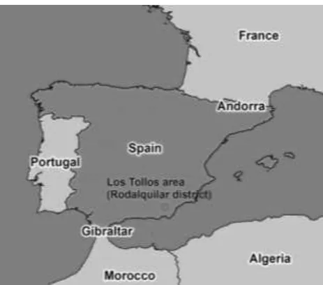
Los Tollos area is a part of the Rodalquilar district in the Sierra del Cabode Gata, in south-eastern Spain (Figure 1). The area has volcanic rocks of different compositions form pyroxene-bearing andesites to rhyolites (Arribas et al, 1995). The intense alteration of rocks is due to two reasons viz., volcanic geothermal activity known as hypogene alteration and chemical weathering also known as supergene alteration. Because of volcanic activity and alterations, there are deposits of different minerals and large-scale mining of alunite has taken place in the area.
Figure. 1. Location of study area
2.2 Dataset Used
We used an airborne hyperspectral image obtained from the HyMap sensor, having 126 contiguous spectral bands, covering 0.45 – 2.5µm of electromagnetic spectrum at spectral resolution
Table 1. HyMap instrument details (Cocks et al, 1998)
between 15 – 20nm. Spectral coverage is nearly continuous in the SWIR and VNIR regions with small gaps in the middle at atmospheric water absorption bands (1.4 and 1.λ m) (Table 1). The HyMap image utilized is a sub-scene of area 2.87 km2, covering the Los Tollos area. We have considered it because the area is mostly covered with the three minerals viz., alunite, illite and kaolinite. The study area was imaged on 11.07.2003 in 126 narrow bands, from 0.45 to 2.48 m with a pixel size of 5m.
2.3 Field Data
Field spectra from some parts of the study area were collected using the Analytical Spectral Device (ASD) fieldspec-pro spectrometer, which covers the wavelength range between 0.35–2.50 m with a spectral resolution of 3nm at 0.7 m and 10nm at 1.4 m and 2.1 m. The spectral sampling interval is 1.4nm in 0.35–1.05 m wavelength range and 2nm in the 1.0–
2.5 m wavelength range. For validating the classification, there
were 17 validating points available, of those 7 points were of alunite, 7 for kaolinite and 3 points for illite mineral. Figure 2, shows the field data collection points in the study area.
Figure. 2. HyMap image of the study area showing the position of validation points
Spectrum Wavelength Range
( m) Bandwidth (nm)
Spectral Sampling
(nm)
VIS 0.45-0.89 15-16 15
NIR 0.89-1.35 15-16 15
SWIR1 1.40-1.80 15-16 13
SWIR2 1.95-2.48 18-20 17
IFOV 2.5m along track 2.0m across track FOV 60º(512 pixels)
Swath 2.3km at 5m IFOV
4.6km at 10m
2.4 Methodology
2.4.1 Proposed SVMDRC framework
The work flow, shown in figure 3 is described here. An airborne hyperspectral image of the study is selected and was preprocessed by performing atmospheric and geographic corrections. The preprocessed image is then subjected to SVM classification, with set of endmembers of each class taken from the image. The same training set and image are then subjected to SVMDRC framework. The classified images obtained from both the classifications are compared for accuracies by validating data. Separability analysis was performed to test the influence of dimensionality reduction by calculating the separation between the classes of the image before and after dimensionality reduction.
The work methodology is divided into two parts, SVMDRC and SVMC. SVMDRC is the work which includes the developing of the framework and applying it on the hyperspectral image, and SVMC part is performing SVM classification on the hyperspectral image using the same training samples used by SVMDRC. The difference between the SVMDRC and is that, in the SVMC no dimensionality reduction is performed and in the SVMDRC dimensionality reduction is performed along with classification. Training samples are taken from the image, which are the endmembers of the class, which has to be classified. With the training samples provided, the SVM classifier decides the hyperplane and the support vectors are generated to separate the classes for classification.
Figure. 3. Methodology.
2.4.2 Pre-processing
The HyMap scene was atmospherically corrected by using parametric geocoding procedure (PRAGE), Airborne Atmospheric, and Topographic Correction Model (ATCOR4) software by German Aerospace Centre. Where the scanning geometry of the image has been reconstructed by using PRAGE with the aid of the pixel positions, altitude and terrain elevation data (Schlapfer et al, 2002).
2.4.3 Dimensionality reduction using eigen decomposition
Dimensionality reduction is performed by eigen decomposition of the covariance matrix, where the covariance matrix of the original image is calculated and the eigen values and the eigen vectors are computed for each band. The scores for each band are calculated and the corresponding transformed components are obtained. These components have the data in the order of decreasing variability. As per the above statements, it means that the first component obtained will have the data, which have maximum variability, and so the variability decreases. In this way, the initial components will have the maximum amount of data. However, selecting the optimum number of transformed bands for obtaining the dimensionally reduced image is real task.
2.4.4 Intrinsic dimensionality calculated using modified broken stick rule
After the reduced bands of the complete hyperspectral image are obtained and their variability are calculated, an optimum number of bands must be selected for further processing, such that the selected data have most of the variability. These numbers of optimum bands selected represent intrinsic dimensionality of the image. Traditionally it is calculated by finding the number of bands by calculating the number of bands falling into the threshold set on the cumulative percentage variability of the image. This is generally set between 98 – 99% of variability. By this method, the intrinsic dimensionality achieved would be between 2 to 5. This would give better results if the number of bands were low. However, if a dataset like hyperspectral image are used which have very high dimensions the intrinsic dimensionality achieved by that above method is not satisfactory. As the dimensions are very high, such a low intrinsic dimensionality will not be promising and the complete feature detection chances would be less. Therefore, by setting a bigger threshold could increase the chance of apt feature selection and detection form the hyperspectral image. However, the threshold which must be set cannot be an arbitrary value.
Radial basis function (RBF) kernel is used in SVM. For dimensionality reduction the complete data is transformed into the lesser dimensions using the eigen decomposition method.
2.5 Influence of dimensionality reduction on feature extraction
The influence of dimensionality reduction on feature reduction is assessed by calculating the distance (feature separability) between the classes before and after dimensionality reduction Jeffries-Matusita (JM) distance method was used to calculate the separability, which gives the distance (class separability) between two distributions. Consider two distributions p(x|ω_i) and p(x|ω_j) which are polynomial populations each having N classes. The sum of the values is equal to 1 as per laws of probability.
The JM distance is defined as in equation
It is the measure of average distances between two class probability density functions.
If the classes are normally distributed then the distance is given by the following equation
where, B is Bhattacharyya distance. The importance of the exponential factor is that it gives the decreasing weight for the increasing separability between the spectral classes. The values of the distance are scaled between 0 and 2.0. The distance with a value 2.0 indicates that the classes are 100% separable and a value 0 that the classes are not separable (Richards et al, 2006).
2.6 Proposed SVMDRC framework
The SVM based dimensionality framework developed in this study is an integration of dimensionality reduction procedure based on eigen vector analysis, automatic selection of optimal transformed components and simultaneously classification of hyperspectral image using non-linear SVM. The proposed framework has been mathematically briefed as follows:
Let X(x_i,y_i ) where i=1,…,n∈R^2is the input data and X^T
(y_i,x_i ) where i=1,…,n∈R^2 be the transposed matrix of the
input data.
Calculate the covariance of the data denoted by K
Apply eigen decomposition to K and obtain the eigen vector and eigen values
where V is the eigen values matrix and D is the eigen vector Matrix.
Sort the values of V in the decreasing order
where p=1,…,m and q=1,…,l and 1≤l≤m
for j=1,2,…,k and
where,
is a fair share of total variability represented by _j within
_j,…, _p. J gives the intrinsic dimensionality.
where c is the normalized value.
The dimensionally reduced and projected data is
Applying SVM for the projected data
where i=1,2,…l
where Φ() is the Radial Basis Function
3. RESULT AND DISCUSSION
3.1 Dimensionality reduction and classification
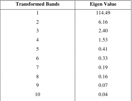
The framework designed performs dimensionality reduction and classification of the hyperspectral image in a single process. In the process, the covariance of the image is calculated, over that eigen decomposition is performed which produces eigen vectors and eigen values of the image. They are also known as scores and loadings. A list of eigen values for each band are generated. Table 2, depicts the eigen values of the first ten bands of the image. The remaining values are very small hence, they are not displayed. Looking at the variance values of the bands in the image, the first five bands contain 98.8% of data in it. So, in the traditional way the intrinsic dimensionality of the reduced transformed image is considered to be 5. Nevertheless, this is not true in the case of hyperspectral imagery. Due to high correlation between the bands and the data shown in the first 5 bands as per the traditional way is limited. To overcome this, modified broken stick rule is implemented to calculate the intrinsic dimensionality of the reduced image.
Transformed Bands Eigen Value
1 114.49
2 6.16
3 2.40
4 1.53
5 0.41
6 0.33
7 0.19
8 0.16
9 0.07
10 0.04
Table 2. Eigen values of the first 10 transformed bands of the image.
3.2 Modified Broken Stick rule
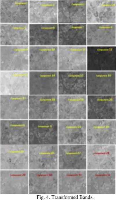
By the MSBR method, the intrinsic dimensionality is the number of dimensions out of total dimension of the image, which is calculated and found out to be 27 for the dataset used in this study. This is how intrinsic dimensionality is calculated and the reduced data with 27 bands is classified. It is to be noted that the complete process of dimensionality reduction and classification is a single stepped processes, but the intrinsic dimensionality can be retrieved just for knowledge by passing the arguments in the code. In the figure 4, the transformed components selected by the broken stick rule along with remaining noisy transformed bands are displayed. After the 27th transformed band the noise content in the image is increased drastically, even though the transformed band have information the noise content is dominating it, which could be visually interpreted.
Fig. 4. Transformed Bands.
3.3 Comparison of SVMDRC and SVM Classification
The framework produces a raster image, which is dimensionally reduced and classified. Both SVMDRC and SVMC part gives a classified image as output. However, the differences between them are one is dimensionally reduced and other is not dimensionally reduced and the other difference is the accuracy of the classification. The accuracy is checked by performing accuracy assessment.
The figures 5 and 6 shows the outputs obtained by two different processes of classification using SVM one with dimensionality reduction and other without dimensionality reduction. In dimensionality reduction, the intrinsic dimensionality of the image is estimated and calculated by modified broken sick rule method and the value is observed to be 27. The first 27 reduced bands are used for classification of the image. The dimensionally reduced and classified image is shown in the figure 5.
Figure. 5. SVMDRC classified image
Figure 6 shows the image obtained by performing SVM classification without dimensionality reduction of the hyperspectral image. The training of the SVM classifier is performed with the same training sets used for SVM dimensionality reduction and classification process, to make sure that same type of classification parameters are considered.
Figure 6. SVM classified image without dimensionality reduction.
The areas of classes were calculated for both the classified mineral maps. By performing SVM on the image the area of the class alunite was 127.44 hectares, illite was 22.23 hectares, kaolinite was 59.45 hectares and unclassified area was 59.45 hectares. Whereas, by applying the SVMDRC the areas obtained were for alunite 118.3825 hectares, illite was 15.48 hectares, kaolinite was 58.712 hectares and unclassified area was 74.9675 hectares.
3.3.1 Validation:
Validation is an important step, which gives the true assessment of the results obtained, i.e., it gives the accuracy of the classified image. Validation data has been collected from different parts of the study area. By this validation data also known as ground truth data, validation of the classified image is performed.
Collection of field spectra from some parts of the study area (shown in figure 2) was performed during the over-flight using the Analytical Spectral Device (ASD) fieldspec-pro spectrometer. This spectrometer covers the 0.35–2.50 m wavelength range with a spectral resolution of 3nm at 0.7 m and 10nm at 1.4 m and 2.1 m. The spectral sampling interval is 1.4nm in the 0.35–1.05 m wavelength range and 2nm in the
1.0–2.5 m wavelength range.
As shown in Table 3, 17 validation points were available in the study area. Of the available 17 validating points, 7 points are of alunite, 7 for kaolinite and 3 points for illite mineral.
Accuracy is assessed calculating the confusion matrix between the ground truth data and the classified image. This process is performed on both the classified images. The results of the SVM classified image and dimensionally reduced and classified image are given in the tables 4 and 5 respectively.
From Table 4, which displays the accuracy assessment of SVM classified image, the overall accuracy of classification is 64.70% where the individual producer’s accuracy of the classes alunite, kaolinite and illite are 85.71%, 42.85% and 66.66% respectively with a kappa coefficient value of 0.43, whereas from table 4, which displays the accuracy assessment of SVMDRC classified image, the overall accuracy of classification is 82.35% but the individual producer’s accuracy of the classes alunite, kaolinite and illite are 85.71%, 85.71.85% and 66.66% respectively with a kappa coefficient value of 0.72. There is an increase in the overall accuracy of classification. This shows that even though SVM takes care of dimensionality
of the image, performing dimensionality reduction will increase the classification accuracy.
Table 3. Reference data from the ground
Confusion Matrix
Table 4. Validation result obtained for SVM classified image and dimensionally reduced and SVM classified image
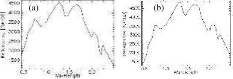
The individual accuracies of the classes was increased. The major change was with the class kaolinite. The producer’s accuracy of kaolinite was 42.85% before dimensionality reduction was performed and after it became 85.71%. Before dimensionality reduction, kaolinite was classified into illite class. This is because of high spectral similarity between both the classes. The spectra of kaolinite and illite classes showed in the figure 7 (a) and (b) respectively, give a visual estimate of spectral similarity between them. There is only a small change in the spectral signatures between the classes. This has led to misclassification of pixels. By performing dimensionality reduction the separation between the two classes have increased leading to better classification. The classification accuracy of the kaolinite mineral has led to the drastic change in the levels of accuracy and the framework has successfully separated them and gave a better level of classification accuracy.
Figure. 7. Spectral profile of (a) Kaolinite and (b) Illite
3.4 Influence of dimensionality reduction on feature extraction
For finding out the influence of dimensionality reduction on feature extraction, separability analysis between the classes was performed by using JM distance method. They are displayed in tables 6 and 7. It was observed that before dimensionality reduction, there was a moderate separability between the classes. The value was 1.34 and the separability values of remaining class pairs were. After dimensionality reduction, the same tests were performed on the image and the vales of all the class separability between the class pair kaolinite-illite was 1.38 and the remaining classes were between 1.3 and 1.41, which is a measure of good separability. Hence, it is shown that performing dimensionality reduction shows a positive increase in index on the feature extraction, which increases the separation between the classes, leading to better classification. The separation of the kaolinite class has increased after dimensionality reduction, which increased the producer’s accuracy of kaolinite class leading to increase in the overall classification accuracy.
Mineral Alunite Illite Kaolinite
Alunite 0.0 1.39 1.41
Illite 1.39 0.0 1.34
Kaolinite 1.41 1.34 0.0
Table 6. JM distances between the class pairs before dimensionality reduction.
Mineral Alunite Illite Kaolinite
Alunite 0.0 1.39 1.41
Illite 1.39 0.0 1.34
Kaolinite 1.41 1.34 0.0
Table 7. JM distances between the class pairs after dimensionality reduction.
4. DISCUSSION AND CONCLUSION
A framework for dimensionality reduction and classification using SVM was developed and implemented on the airborne hyperspectral image for classification of minerals in the study area. Hyperspectral image classified by the framework has shown better accuracy than the classified using SVM alone. This indicates that SVM take care of dimensionality to a limited degree. Hence, performing dimensionality reduction is a compulsory step for processing the hyperspectral images. Separability analysis by JM distance method gave an interesting result. Before dimensionality reduction of the image, the separability analysis showed that two pairs of classes were having very less separability between them. This was the reason for the intermixing of the class pixels. There was poor separability between kaolinite and illite. Once dimensionality reduction is performed on the image the separability has increased between the class pair kaolinite and illite. The confusion matrix shows that the misclassification rate has decreased and hence the classification accuracy increases. This result gives an impression that if dimensionality reduction is performed the chances of having misclassified pixels will low.
This work also shows that dimensionality reduction shows a positive impact on feature extraction, where the separation between the classes increases after dimensionality reduction is performed. Performing SVM on the hyperspectral image have
Station X Y Determinant
LT04-25 -2.01939 36.86044 Alunite LT04-15 -2.02209 36.86041 Alunite LT04-11 -2.02546 36.86038 Alunite LT04-12 -2.02840 36.86088 Kaolinite
LT04-04 -2.03227 36.86052 -
LT04-10 -2.02015 36.86222 Alunite LT04-20 -2.02335 36.86220 Alunite LT04-6 -2.02602 36.86299 Alunite LT04-3 -2.02986 36.86269 Alunite LT04-14 -2.02179 36.86419 Kaolinite LT04-17 -2.03001 36.86495 Kaolinite LT04-23 -2.03286 36.86401 Kaolinite
LT04-7 -2.02039 36.86642 Illite LT04-1 -2.02394 36.86616 Kaolinite LT04-24 -2.02757 36.86698 Illite
LT04-9 -2.03212 36.86648 Kaolinite
(b) (a)
given an accuracy of 64.70% whereas accuracy after the framework is applied was 82.35%. There are certain advantages of using a unified framework. First is that the process of working will become shorter. Instead of a two-step process, the work is performed in a single step, this makes the work process faster and more efficient, the results of this research work have proved this point. The second advantage is the usage of SVM in the framework. The framework is completely written in open-source software hence it is accessible to the scientific community for the usage and further improvements.
ACKNOWLEDGEMENTS
Authors acknowledge Dr. C.A. Hecker, and Dr. F.J.A. Van Ruitenbeek, for providing with hyperspectral image and essential field data. Special thanks to Dr. V.A. Tolpekin. Author would like to thank Prof. dr. ir. Alfred Stein, Dr. S.K. Srivastav, Mr. PLN Raju for their guidance, support and encouragement.
REFERENCES
Arribas A. Jr, Cunningham C.G., Rytuba J.J. , Rye R.O., Kelley W.C., Podwysocki M.H., McKee E.H. and Tosdal R.M., 1995, “Geology, geochronology, fluid inclusions and isotope geochemistry of the Rodalquilar gold alunite deposit, Spain,” Economic Geology, 90, 795–822.
Bajorski P., 200λ, “Does Dimensionality work in hyperspectral
images?” In Proc. SPIE, Algorithms and technologies for
Multispectral, Hyperspectral and Ultraspectral Imagery XV
Bajorski P., 2011, “Second moment linear dimensionality as an alternative to virtual dimensionality,” IEEE Transactions on Geosciences and Remote Sensing, 49(2), 672-678 (2011).
Burgers K., Fessehatsion Y., Rahmani S., Seo J., and Wittman T.,2009, “A Comparative Analysis of Dimension Reduction Algorithms on Hyperspectral Data,” LAMDA Research Group.
Cocks T., Jenssen R., Stewart W.I. and Sheilds T., 1λλ8, “The HyMap airborne Hyperspectral sensor: The system, calibration and performance,” First EARSEL workshop on imaging spectroscopy, Zurich.
Cortes C. and Vapnik V., 1λλ5, “Support-vector Networks,”
Machine Learning, 20(3), 273–97.
Jackson J.E., 2003, A User's Guide to Principal Components, Wiley.
Schlapfer D. and Ritcher R., 2002, “Geo-atmospheric processing of airborne imaging spectrometry data. Part 1: parametric orthorectification,” International journal of Remote Sensing, Vol 23 (14), 2609 – 2630, (2002).
Soman K.P, Ajay V., and Loganathan R., 2009, Machine Learning with SVM and other Kernel Methods, Prentice-Hall India (2009).
Richards J.A. and Jia X., 2006, Remote Sensing Digital Image Analysis- An Introduction, 4thEdition, Springer.
Yang B., 200λ, “SVM-Induced Dimensionality Reduction and
Classification,” In proceedings of Second conference on intelligent computation technology and Automation, 275–278.