QUALITY ASSESSMENT OF SELF-CALIBRATION WITH DISTORTION ESTIMATION
FOR GRID POINT IMAGES
Z. Franjcica, b,∗, J. Bondesona a
Qualisys AB, Gothenburg, Sweden - (zlatko.franjcic, johan.bondeson)@qualisys.se bt2i Lab, Chalmers University of Technology, Gothenburg, Sweden
Commission VI, WG VI/4
KEY WORDS:Self-Calibration, Gr¨obner basis, Bundle Adjustment, Image Distortion, Planar Pattern, Performance Analysis
ABSTRACT:
Recently, a camera self-calibration algorithm was reported which solves for pose, focal length and radial distortion using a minimal set of four 2D-to-3D point correspondences. In this paper, we present an empirical analysis of the algorithm’s accuracy using high-fidelity point correspondences. In particular, we use images of circular markers arranged in a regular planar grid, obtain the centroids of the marker images, and pass those as input point correspondences to the algorithm. We compare the resulting reprojection errors against those obtained from a benchmark calibration based on the same data. Our experiments show that for low-noise point images the self-calibration technique performs at least as good as the benchmark with a simplified distortion model.
1. INTRODUCTION
Estimating the position and orientation of a camera along with its intrinsic properties is a fundamental problem in computer vi-sion. In three-dimensional machine vision, this goal is tradition-ally achieved by calibrating a camera model with the help of 2D images of reference points, whose 3D coordinates are known rel-ative to some coordinate system (Tsai, 1987, Wei and Ma, 1993, Heikkila and Silv´en, 1997).
Recently, self-calibration methods have become popular (Hart-ley, 1997, Triggs, 1998, Li and Hart(Hart-ley, 2005). Those techniques do not use a calibration object, but rather exploit structural fea-tures of a static scene viewed from different positions. Corre-spondences across the different views then provide constraints used to derive the model parameters.
An interesting class of self-calibration techniques are those that try to minimize the number of correspondences necessary. Very recently, techniques originally described by (Triggs, 1999) were used by (Josephson and Byrod, 2009), and shortly after by (Buj-nak et al., 2011) to state minimal problems that include modeling of non-linear effects, such as radial distortion.
In this paper we compare how the method by (Bujnak et al., 2011), used for self-calibration, fares against a traditional calibra-tion method (Zhang, 2000) in terms of reprojeccalibra-tion error. In order to do so, we use images of a calibration object, a regular grid of circular markers. Thus, we already provide 3D point coordinates both to the calibration technique and also to the self-calibration method. In this scenario, the traditional calibration method serves as a benchmark or “gold standard”. We consider this to be justi-fied, as the method by (Zhang, 2000) is implemented as the cal-ibration method of choice in some form or another in a variety of (open-source) software packages, including such popular soft-ware as OpenCV (Bradski and Kaehler, 2008) and the MATLAB Camera Calibration Toolbox by (Bouguet, 2004).
Since the two approaches are targeted at different applications, there do not seem to be many comparisons across them. The work
∗Corresponding author
by (Devernay and Faugeras, 2001) compares a self-calibration technique against a regular calibration, but they do not use a minimal solver that models radial distortion. In (De Villiers et al., 2008), different distortion models and numerical optimiza-tion techniques are compared, but only the tradioptimiza-tional calibraoptimiza-tion technique is used in any of the experiments.
1.1 Contributions
The main contributions of this paper are
• Applying the algebraic minimal problem solver by (Buj-nak et al., 2011) and the associated proposed self-calibration method for images of only a few, but confirmed, co-planar points arranged in a grid pattern, and verifying its feasibility for this type of task up to a specific qualitative accuracy.
• Comparing that self-calibration against a benchmark cali-bration method (Zhang, 2000) based on bundle adjustment with respect to reprojection error.
• Using the best solutions from the self-calibration as initial values for bundle adjustment and comparing the resulting optimization result with the default of using a constant initial guess chosen in advance.
2. CAMERA MODEL
The general model of a camera used in this paper is the pinhole camera model (Hartley and Zisserman, 2003). The projection equation in the pinhole model can be written as
sx=
fx γ cx
0 fy cy
0 0 1
| {z }
M
R | tX. (1)
camera intrinsics matrix capturing the focal length along thex andycoordinates of the image,fxandfy, and the camera’s prin-cipal point(cx, cy), while the parameterγdescribes the skewness of the two image axes. Since the projection is only defined up to scale, an arbitrary scale factorsis included in the equation.
For the remainder of the paper we assume zero skew, as was done by (Bujnak et al., 2011) and (Zhang, 2000).
3. DISTORTION MODEL FOR THE
SELF-CALIBRATION
The method by (Bujnak et al., 2011) uses the division model (Fitzgibbon, 2001) for radial distortion, which is given by
is the radial distortion coefficient, andrd2=x
2
d+y
2
d.
In order to formulate a minimal problem, three more simplifi-cations are made to reduce the degrees of freedom. Firstly, the principal point is set to the image center. Secondly, the center of distortion is set to the principal point, and thus also to the image center. And lastly, the aspect ratio is set to1. With these assump-tions and by including the radial distortion from Equation (2) into the model from Equation (1), the projection can be described as
s
In their work, (Bujnak et al., 2011) describe two different param-eterizations for the unknowns in this equation system depending on whether the 3D points are coplanar or not. In each case, the re-sult is a polynomial equation system that can be solved efficiently using the Gr¨obner basis method (Cox et al., 1998). A detailed de-scription of the method is beyond the scope of this paper, and we refer the reader to (Stew´enius, 2005) for a background on the theory of Gr¨obner basis solvers and its application to computer vision.
4. DISTORTION MODEL FOR THE BENCHMARK
CALIBRATION
The work by (Brown, 1966, Brown, 1971) proposed a model for mapping a distorted image point to a point in an image obtained from a distortion-free projection. In (Wei and De Ma, 1994) it is shown that the same functional form can be used for the reverse mapping. The reverse mapping is also used by (Zhang, 2000) and can be described as
torted image point,(˜xu,y˜u)is the undistorted point’s relative po-sition to the center of distortion(xc, yc),kiis theithradial
distor-tion coefficient andpjis thejthdecentering distortion coefficient, andr2
As for the self-calibration and as (Zhang, 2000), we assume that the center of distortion is the same as the principal point, thus we set(xc, yc) = (0,0). Furthermore, and again in line with (Zhang, 2000), we only consider the first two coefficients for radial dis-tortion (k1,k2). But additionally, we include the first two coeffi-cients for decentering distortion as (Wei and De Ma, 1994) did.
To determine the distortion coefficients, along with focal lengths
(fx, fy)and principal point(cx, cy)from Equation (1), givenn images ofmco-planar points the following optimization problem can be stated:
Here,bjis the parameterization of the camera in viewj,Qis the modeled projection function,Xiare pointi’s 3D coordinates and xijare pointi’s image coordinates in viewj.
To solve this equation numerically, the Levenberg-Marquardt al-gorithm (Levenberg, 1944, Marquardt, 1963) can be used, which is the method also suggested by (Zhang, 2000).
5. COMPARING THE SELF-CALIBRATION AND THE
BENCHMARK CALIBRATION MODELS
In order to make the two different models somewhat comparable, we adapt the benchmark’s model by setting the principal point to the image center and assuming an aspect ratio of1as in the right-hand side of Equation (3). We also simplify the benchmark’s distortion model from Equation (4) to not account for decentering distortion, and only include the first radial distortion coefficient.
Through these changes, we get the same number of parameters in both models. In particular, we can directly compare the focal length, rotation and translation estimates from both models. The only parameter not directly comparable is the radial distortion coefficient. However, (Fitzgibbon, 2001) showed that these two radial distortion models approximate the true distortion function nearly equally well.
As the benchmark calibration method (Zhang, 2000) assumes im-ages of points located in a single two-dimensional plane, we are restricted to using images of coplanar points, only. For our anal-ysis and experiments, we consider points arranged in a regular two-dimensional grid pattern. As for the images of the grid pat-tern, we initially normalize all image coordinates by scaling them with a factor of
scale= 2
max(width, height)−1, (6)
so that all image coordinates are mapped between minus one and one (Josephson and Byrod, 2009). This way, the analysis is inde-pendent of image size.
points in the same image, instead of sampling any set of 4 points as a traditional RANSAC approach would suggest. Each sampled 4-point configuration is fed to the minimal solver to obtain the model parameters. We calculate for each point in the same im-age the reprojection error under the model and determine which points are inliers. The criterion for a point being an inlier is based on the results from the benchmark calibration with the simplified model for the exact same image: if the reprojection error for a point is less than3times the maximum reprojection error over all points from the same image for the benchmark calibration, then the point is considered an inlier. From all sampled 4-point config-urations for a given image, we keep the solution with the highest number of inliers, and, as a secondary criterion, the lowest aver-age reprojection error over all inliers. We repeat this procedure for all images.
For the benchmark calibration we minimize the reprojection func-tion given in Equafunc-tion (5) using the Levenberg-Marquardt algo-rithm. We perform the minimization twice: once employing the distortion model from Section 4., which we subsequently refer to as thefull model, and a second time using the simplified model as described previously in this section. Instead of single images as for the RANSAC-like method described above, we divide all im-ages into sets and apply the Levenberg-Marquardt algorithm on each set individually. But as before, we obtain the reprojection errors for all 3D-to-2D point correspondences, as well as esti-mates for focal length, distortion coefficients, rotation and trans-lation. Note however, that, for a given set of input images, the benchmark calibration only estimates a single focal length for the complete set, while the self-calibration technique gives an esti-mate for each image individually. The same holds true for the respective radial distortion coefficients.
6. EXPERIMENTAL RESULTS
6.1 Measurement acquisition
For the image acquisition we used two Qualisys Oqus 3+ cam-eras, one equipped with a 25mm lens, the other with a 50mm lens. The 25mm lens is shipped by default with the camera. We chose to test the 50mm lens as well because this lens is of higher quality than the 25mm one, exhibiting less pronounced distortion characteristics. This fact, we hypothesized, would allow for con-clusions about the relative performance of the calibration meth-ods depending on the distortion characteristics of the lens.
The Qualisys Oqus cameras are usually used for 3D motion cap-ture, recording infrared light reflected from or actively emitted by spherical or circular marker objects. The reason to choose those cameras is that we wanted to take images of single points without sophisticated image feature extraction. Since the motion capture cameras are optimized to record the relatively small markers, the feature extraction task is simplified to finding (nearly) circular spots on the image. Since we wanted to have single points, we used the cameras built-in functionality to calculate the centroids of detected markers to obtain subpixel coordinates of the image points.
To capture images of co-planar points, we used a plate with cir-cular retro-reflective markers arranged in a regular4×5grid, so that the distance between neighboring markers along a particu-lar dimension is the same. We used the camera-calculated image coordinates of the marker centroids for our final analysis. Fig-ure 1 shows a color pictFig-ure of the plate, while FigFig-ure 2 shows an image of the markers taken by the Qualisys Oqus camera in marker-detection mode.1
Figure 1: The plate used for calibration, with4×5circular retro-reflective markers arranged in a regular grid pattern.
Figure 2: A visualization of the markers seen and identified by the Qualisys Oqus 3+ camera.
For each of the two lenses, we took images of the plate from different angles and at two different distances from the cameras, such that the image points were distributed over the entire im-age sensor for both distances. The two distances were adapted according to each lens’ approximate focal length. With up to20
points per image, we got105111points in5267images for the 25mm lens, and76299points in3866images for the 50mm lens.
6.2 Self-calibration versus benchmark calibration
We divided the data for each lens into different, similarly sized sets, yielding7sets for the 25mm lens and8sets for the 50mm lens. For each set, we performed a benchmark calibration and recorded the reprojection error for each point in each image. We ran the calibration for both the simplified model as described in Section 5. as well as the full model described in Section 4.
We then ran the self-calibration on the same set, using the sam-pling approach described in Section 5. For each image,30 sam-pling iterations were performed where a minimal set of4points was selected. We determined the number of inliers and kept track of the model with the largest number of inliers. If two models gave rise to the same number of inliers, we only considered the one resulting in the smaller average reprojection error over all in-liers. Concurrently, we also recorded the individual reprojection errors for all inlier points for that model.
Figure 3 shows the empirical mean and standard deviation of the number of inliers given the number of sampling iterations over all images for both lenses. For most images, the inliers included all points after the first iteration step. All the points in all images were determined to be inliers after the maximum number of itera-tions. This is an indication that the acquired point images contain very little noise, which can be attributed to the high-fidelity grid pattern and the fact that only nearly-circular features had to be extracted from the images. The lower mean and higher variance of the number of inliers for the 50mm lens can possibly be ex-plained by the observation that in general it is better not to model
1
0 5 10 15 20 25 Iterations
0 5 10 15 20
In
lie
rs
(a)
0 5 10 15 20 25
Iterations 0
5 10 15 20
In
lie
rs
(b)
Figure 3: RANSAC-like procedure during self-calibration: Mean and standard deviation of number of inliers given the number of sampling iterations for the 25mm lens (a) and the 50mm lens (b). The standard deviation is truncated towards the top, as the num-ber of inliers can be at most20(the number of markers in the grid pattern).
lens distortion if the effects are negligible (Josephson and Byrod, 2009), which we assume is the case for this high-quality lens we used.
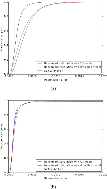
Figure 4 displays for both lenses the cumulative distribution of re-projection errors for all (inlier) points over all images for both the benchmark calibration (simplified and full model) and the self-calibration. Based on the visual representation, it seems that, for the 25mm lens, the self-calibration and the benchmark cali-bration with the simplified model perform similarly well, while the benchmark calibration with the full model performs better. In order to validate this impression, we performed a t-test for paired samples, pairing the point-wise reprojection errors of the three methods against one another. We observed a significant difference (p <0.001) for any two, with the benchmark calibra-tion with the simplified model actually performing worse than the self-calibration with respect to average reprojection error. For the 50mm lens, the figure does not reveal a clear difference between the three techniques. Again, a t-test for paired samples indicated a significant difference (p < 0.001) between any two, with the self-calibration having the lowest average reprojection error, and the benchmark calibration with the full model the highest one. As mentioned before, it seems that modeling the negligible dis-tortion effects for the 50mm lens is not beneficial, thus a sim-pler model will probably “cause less harm” than a more elaborate one. A reason for the self-calibration method performing better
than the benchmark calibration with the simplified model irre-spective of the lens used could be that the model parameters are fitted for each image individually for the self-calibration method, while the parameters for the benchmark calibration are fitted to a set of multiple images.
0.0000 0.0005 0.0010 0.0015 0.0020 Reprojection error
0.0 0.2 0.4 0.6 0.8 1.0
Fra
cti
on
of
all
po
ints
Benchmark calibration with full model Benchmark calibration with simplified model Self-calibration
(a)
0.0000 0.0005 0.0010 0.0015 0.0020 Reprojection error
0.0 0.2 0.4 0.6 0.8 1.0
Fra
cti
on
of
all
po
ints
Benchmark calibration with full model Benchmark calibration with simplified model Self-calibration
(b)
Figure 4: Cumulative distribution of the reprojection error values for all points across all views for the benchmark calibration using the full model, the benchmark calibration using the simplified model, and the self-calibration for both the 25mm lens (a) and the 50mm lens (b).
6.3 Self-calibration combined with benchmark calibration
In this experiment, we used the best estimate, in terms of repro-jection error, of focal length and radial distortion from the self-calibration for each set of images used by the benchmark cali-bration. This best estimate was set as the initial guess for the Levenberg-Marquardt algorithm within the benchmark calibra-tion with the full model for the respective set of images.
We observed that the benchmark calibration is rather unsensitive to the choice of intial guess, as we got the exact same final esti-mates for the extrinsic and intrinsic parameters as when using a constant default guess. We attribute this to the robustness proper-ties of the Levenberg-Marquardt algorithm.
7. LIMITATIONS
Both the division model in Equation (2) and the simplified model for the benchmark calibration make use of a single radial distor-tion coefficient. For the lenses used in our experiments this was sufficient, as the lenses would either exhibit moderate barrel or pincushion distortion, but not a combination of both. However, our results cannot be generalized to lenses with complex distor-tion, and, in fact, we would expect the calibration methods based on those models to perform significantly worse in such cases.
As feature extraction and marker centroid calculation inside the Qualisys Oqus cameras is implemented by proprietary algorithms, we cannot assess the theoretical robustness properties and error characteristics of that measurement step.
8. CONCLUSION AND FUTURE WORK
In this paper, we presented a comparison of a specific camera self-calibration method that includes modeling of radial distortion to a benchmark calibration method to assess the former’s relative performance in terms of reprojection error for images of a regular grid of points.
We showed that for this particular case with high-fidelity images taken from a regular grid of circular markers, the self-calibration scheme produced lower average reprojection errors compared to the benchmark calibration with a simplified model, for both a 25mm and a 50mm lens. We also used the focal length and radial distortion parameter pairs estimated by the self-calibration tech-nique as initial guess for the benchmark calibration with the full model, but observed that the optimization yielded the exact same final estimates for both intrinsic and extrinsic parameters as when using a constant default guess.
Future work could show whether running the benchmark calibra-tion on a per-image basis results in better performance than run-ning it on sets of images — something we expect, as we think it is an example of overfitting. We also suggest a more comprehen-sive study comparing a variety of self-calibration and offline cal-ibration methods to better understand their relative performance characteristics under different conditions. Finally, as an alterna-tive to using the reprojection error as calibration quality indicator, deviations of reconstructions from 2D images of a ground-truth 3D scene whose geometry is known to a very high accuracy could be calculated and compared across the different reconstructions.
ACKNOWLEDGEMENTS
We would like to thank Alexandru Dancu. This work was sup-ported by the People Programme (Marie Curie Actions) of the European Union’s Seventh Framework Programme FP7/2007– 2013/ under REA grant agreement no. 289404.
REFERENCES
Bouguet, J.-Y., 2004. Camera calibration toolbox for matlab.
Bradski, G. and Kaehler, A., 2008. Learning OpenCV: Computer vision with the OpenCV library. O’Reilly Media, Inc.
Brown, D. C., 1966. Decentering Distortion of Lenses. Pho-togrammetric Engineering 32(3), pp. 444–462.
Brown, D. C., 1971. Close-range camera calibration. Photogram-metric engineering 37(8), pp. 855–866.
Bujnak, M., Kukelova, Z. and Pajdla, T., 2011. New efficient solution to the absolute pose problem for camera with unknown focal length and radial distortion. In: Computer Vision–ACCV 2010, Springer, pp. 11–24.
Cox, D. A., Little, J. B. and O’shea, D., 1998. Using algebraic geometry. Springer.
De Villiers, J. P., Leuschner, F. W. and Geldenhuys, R., 2008. Centi-pixel accurate real-time inverse distortion correction. In: International Symposium on Optomechatronic Technologies, In-ternational Society for Optics and Photonics, pp. 726611– 726611.
Devernay, F. and Faugeras, O., 2001. Straight lines have to be straight. Machine vision and applications 13(1), pp. 14–24.
Fitzgibbon, A. W., 2001. Simultaneous linear estimation of mul-tiple view geometry and lens distortion. In: Computer Vision and Pattern Recognition, 2001. CVPR 2001. Proceedings of the 2001 IEEE Computer Society Conference on, Vol. 1, IEEE, pp. I–125.
Hartley, R. and Zisserman, A., 2003. Multiple view geometry in computer vision. Cambridge university press.
Hartley, R. I., 1997. In defense of the eight-point algorithm. Pat-tern Analysis and Machine Intelligence, IEEE Transactions on 19(6), pp. 580–593.
Heikkila, J. and Silv´en, O., 1997. A four-step camera calibration procedure with implicit image correction. In: Computer Vision and Pattern Recognition, 1997. Proceedings., 1997 IEEE Com-puter Society Conference on, IEEE, pp. 1106–1112.
Josephson, K. and Byrod, M., 2009. Pose estimation with radial distortion and unknown focal length. In: Computer Vision and Pattern Recognition, 2009. CVPR 2009. IEEE Conference on, IEEE, pp. 2419–2426.
Levenberg, K., 1944. A method for the solution of certain problems in least squares. Quarterly of applied mathematics 2, pp. 164–168.
Li, H. and Hartley, R., 2005. A non-iterative method for correct-ing lens distortion from nine point correspondences. OMNIVIS 2005.
Marquardt, D. W., 1963. An algorithm for least-squares estima-tion of nonlinear parameters. Journal of the Society for Industrial & Applied Mathematics 11(2), pp. 431–441.
Stew´enius, H., 2005. Gr¨obner basis methods for minimal prob-lems in computer vision. Citeseer.
Triggs, B., 1998. Autocalibration from planar scenes. In: Com-puter VisionECCV’98, Springer, pp. 89–105.
Triggs, B., 1999. Camera pose and calibration from 4 or 5 known 3d points. In: Computer Vision, 1999. The Proceedings of the Seventh IEEE International Conference on, Vol. 1, IEEE, pp. 278–284.
Tsai, R. Y., 1987. A versatile camera calibration technique for high-accuracy 3d machine vision metrology using off-the-shelf tv cameras and lenses. Robotics and Automation, IEEE Journal of 3(4), pp. 323–344.
Wei, G.-Q. and De Ma, S., 1994. Implicit and explicit camera cal-ibration: Theory and experiments. Pattern Analysis and Machine Intelligence, IEEE Transactions on 16(5), pp. 469–480.
Wei, G.-Q. and Ma, S., 1993. A complete two-plane camera cal-ibration method and experimental comparisons. In: Computer Vision, 1993. Proceedings., Fourth International Conference on, IEEE, pp. 439–446.